Pin-by-Pin Coupled Transient Monte Carlo Analysis Using the iMC Code

In this article, we present a coupled multi-physics Monte Carlo reactor transient analysis framework implemented in the KAIST Monte Carlo iMC code. In the multi-physics framework, the time-dependent neutron transport calculation and the transient heat transfer analysis are done based on the predictor–corrector quasi-static Monte Carlo method and the three-dimensional finite element method, respectively. Using this high-fidelity analysis framework, we demonstrated the negative temperature feedback effect in two pressurized water reactor (PWR) transient scenarios. First, a 3-D burnable absorber-loaded fuel assembly was considered with all reflective boundary conditions. In this simple problem, a positive reactivity-induced transient was analyzed to characterize the reactor responses in view of the pin-wise power and temperature distribution. Second, the iMC multi-physics analysis is applied to a control rod withdrawal transient in the TMI-1 mini core problem, and detailed time-dependent results were provided and compared with the Serpent/SUBCHANFLOW analysis. In both cases, independent MC runs were performed to quantify the uncertainty of the multi-physics MC transient analysis.

1 Introduction

It is a non-disputable fact that the nuclear reactor is a complex multi-physics system with neutronics, thermal hydraulics, thermo-mechanics, and chemistry interdependency. It is also well-known that a stand-alone physics simulation cannot predict the accurate and reliable dynamic behavior of a given nuclear system, yet many works had been focused on specific physics simulation mostly due to the lack of computational power.

Nowadays, a great portion of researchers in the high-fidelity reactor physics community is focusing on the establishment of a coupled multi-physics analysis framework for transient situations. The time-dependent coupled multi-physics simulations are largely based on neutronics codes with the diffusion or deterministic transport method coupled with reactor hydraulics codes (Fiorina et al., 2015; Cherezov et al., 2020; Park et al., 2020; Wang et al., 2021). In most cases, reactivity feedback effects have been deterministically applied directly to the reactivity, while the feedback constants were independently evaluated from Monte Carlo branch calculations. It is reasonable that the early multi-physics approaches are based on the deterministic neutronics methods as the time-dependent neutronics analysis itself is considered computationally exhaustive.

Despite its computation cost, the explicit Monte Carlo neutron transport method is generally accepted as the most accurate and reliable tool that takes into account various reactor feedbacks that possibly affect the dynamic behavior of a nuclear system in the most explicit way. For pursuing the high-fidelity simulation of transient nuclear systems, a few attempts have been made successfully by Serpent 2 and Tripoli-4 in combination with the SUBCHANFLOW thermal-hydraulics (TH) code (Ferraro et al., 2019; Ferraro et al., 2020a; Ferraro et al., 2020b; Ferraro et al., 2020c; Ferraro et al., 2020d). To our best knowledge, they are so far the only published research outcomes regarding the time-dependent Monte Carlo transport analysis coupled with TH features.

Unlike the Serpent/SUBCHANFLOW framework, the iMC code utilizes intra-pin power distribution for the temperature analysis to provide an enhanced fuel integrity study for a complex fuel element such as the centrally shielded burnable absorber (CSBA) (Nguyen et al., 2019). From a previous study (Kim and Kim, 2020), we found the use of detailed power distribution critical for accurate temperature analysis. We also suggested using the intra-pellet power shape from a separate pin-cell transport calculation in which the effect of neighboring guide thimble can hardly affect the temperature distribution (Kim, 2022).

In this article, we present the iMC simulation results on pressurized water reactor (PWR) problems using the multi-physics coupled scheme. In Section 2, the basic framework of the coupled numerical analysis is introduced. The formulation of the predictor–corrector quasi-static Monte Carlo (PCQS-MC) for the transient neutron transport method, the three-dimensional (3-D) finite element transient heat transfer analysis, and a simplified coolant model for the current analysis are explained. The numerical results are presented in Section 3, showing that the negative temperature effect of fuel and coolant on reactivity successfully moves the given reactor system to a steady state in a reactivity insertion transient.

2 Framework of Transient Multi-Physics Reactor Analysis in iMC

2.1 Predictor–Corrector Quasi-Static Monte Carlo Method

In this section, we discuss the key features for establishing the PCQS-MC method. Guo et al. (2021) implemented the PCQS-MC framework in the RMC based on random samplings of delayed sources within a given time bin and kinetic parameter polynomial fitting method. Meanwhile, Jo and Cho (Jo et al., 2016) used analytic linear interpolation of delayed fission source and exponential transformation method. The iMC adopted the latter approach as we found it mathematically concrete and straightforward to implement.

2.1.1 Transient Fixed Source Iteration for Prediction Step

The time-dependent neutron transport equation includes the time derivative of flux term which is often disregarded in steady-state analyses by defining the multiplication factor. The complete governing equation in the space and time domain requires the following transport equation and precursor concentration equation:

$\begin{array}{c}\frac{1}{v\left(E\right)}\frac{\partial \psi \left(\overrightarrow{r},E,\overrightarrow{\mathrm{\Omega }},t\right)}{\partial t}=-L\psi \left(\overrightarrow{r},E,\overrightarrow{\mathrm{\Omega }},t\right)-T\psi \left(\overrightarrow{r},E,\overrightarrow{\mathrm{\Omega }},t\right)+S\psi \left(\overrightarrow{r},E,\overrightarrow{\mathrm{\Omega }},t\right)\\ +\frac{1}{k_0}\frac{{\chi }_p\left(E\right)}{4\pi }\left(1-\beta \right)F\psi \left(\overrightarrow{r},E,\overrightarrow{\mathrm{\Omega }},t\right)+{\displaystyle \sum _{d=1}^{G_d}\frac{{\chi }_d\left(E\right)}{4\pi }{\lambda }_d{C}_d\left(\overrightarrow{r},t\right),}\end{array}(1)$

$\frac{\partial C_d\left(\overrightarrow{r},t\right)}{\partial t}=\frac{1}{k_0}{\beta }_{d}F\psi \left(\overrightarrow{r},E,\overrightarrow{\mathrm{\Omega }},t\right)-{\lambda }_d{C}_d\left(\overrightarrow{r},t\right),d=1to{G}_d.(2)$

Here, $\psi$ is the neutron flux, $v$ is the energy-dependent neutron speed, $k_0$ is the initial neutron multiplication factor, $\beta$ is the aggregate delayed neutron fraction, $C_d$ is the precursor concentration of delayed group d, ${\lambda }_d$ is the decay constant, $G_d$ is the number of precursor group, and${\chi }_p$ and ${\chi }_d$ are the prompt and delayed neutron fission energy spectrum, respectively. The operators are defined as follows:

$L\psi \left(\overrightarrow{r},E,\overrightarrow{\mathrm{\Omega }},t\overrightarrow{r},E,\overrightarrow{\mathrm{\Omega }},t\right)=\overrightarrow{\mathrm{\Omega }}\cdot \nabla \psi \left(\overrightarrow{r},E,\overrightarrow{\mathrm{\Omega }},t\right),(3)$

$T\psi \left(\overrightarrow{r},E,\overrightarrow{\mathrm{\Omega }},t\right)={\sigma }_t\left(\overrightarrow{r},E,t\right)\psi \left(\overrightarrow{r},E,\overrightarrow{\mathrm{\Omega }},t\right),(4)$

$S\psi \left(\overrightarrow{r},E,\overrightarrow{\mathrm{\Omega }},t\right)={\displaystyle \int d{E}^{\prime }{\displaystyle \int d{\overrightarrow{\mathrm{\Omega }}}^{\prime }{\sigma }_s\left(\overrightarrow{r},E^{\prime }\to E,{\overrightarrow{\mathrm{\Omega }}}^{\prime }\cdot \overrightarrow{\mathrm{\Omega }},t\right)\psi \left(\overrightarrow{r},E^{\prime },{\overrightarrow{\mathrm{\Omega }}}^{\prime },t\right)}},(5)$

$F\psi \left(\overrightarrow{r},E,\overrightarrow{\mathrm{\Omega }},t\right)={\displaystyle \int d{E}^{\prime }{\displaystyle \int d{\overrightarrow{\mathrm{\Omega }}}^{\prime }\nu {\sigma }_f\left(\overrightarrow{r},E^{\prime },t\right)\psi \left(\overrightarrow{r},E^{\prime },{\overrightarrow{\mathrm{\Omega }}}^{\prime },t\right)}},(6)$

where ${\sigma }_t$, ${\sigma }_s$, and ${\sigma }_f$ are the macroscopic total, scattering, and fission cross section, respectively. Applying the implicit Euler scheme in the time domain gives the discretized form of transport equation:

$\begin{array}{c}\frac{\psi \left(\overrightarrow{r},E,\overrightarrow{\mathrm{\Omega }},t_s\right)-\psi \left(\overrightarrow{r},E,\overrightarrow{\mathrm{\Omega }},t_{s-1}\right)}{v\left(E\right)\mathrm{\Delta }t}=-L\psi \left(\overrightarrow{r},E,\overrightarrow{\mathrm{\Omega }},t\right)-T\psi \left(\overrightarrow{r},E,\overrightarrow{\mathrm{\Omega }},t_s\right)+S\psi \left(\overrightarrow{r},E,\overrightarrow{\mathrm{\Omega }},t_s\right)\\ +\frac{1}{k_0}\frac{{\chi }_p\left(E\right)}{4\pi }\left(1-\beta \right)F\psi \left(\overrightarrow{r},E,\overrightarrow{\mathrm{\Omega }},t_s\right)+{\displaystyle \sum _{d=1}^{G_d}\frac{{\chi }_d\left(E\right)}{4\pi }{\lambda }_d{C}_d\left(\overrightarrow{r},t_s\right).}\end{array}(7)$

Rearranging the equation and sorting in terms of time-step flux leads to the following transport equation.

$\left(L+T_{PCQS}-S\right)\psi \left(\overrightarrow{r},E,\overrightarrow{\mathrm{\Omega }},t_s\right)=\frac{1}{k_0}\frac{{\chi }_p\left(E\right)}{4\pi }\left(1-\beta \right)F\psi \left(\overrightarrow{r},E,\overrightarrow{\mathrm{\Omega }},t_s\right)+{\displaystyle \sum _{d=1}^{G_d}\frac{{\chi }_d\left(E\right)}{4\pi }{\lambda }_d{C}_d\left(\overrightarrow{r},t_s\right)}+\frac{\psi \left(\overrightarrow{r},E,\overrightarrow{\mathrm{\Omega }},t_{s-1}\right)}{v\left(E\right)\mathrm{\Delta }t}.(8)$

Here, the modified transport operator for PCQS formulation is defined as follows:

$T_{PCQS}\psi \left(\overrightarrow{r},E,\overrightarrow{\mathrm{\Omega }},t_s\right)=\left({\sigma }_t(\overrightarrow{r},E,t_s)+\frac{1}{v\left(E\right)\mathrm{\Delta }t}\right)\psi \left(\overrightarrow{r},E,\overrightarrow{\mathrm{\Omega }},t_s\right).(9)$

Meanwhile, the delayed neutron source distribution at $t=t_s$ can be determined by integrating Eq. 2 in the given time interval.

$S_d\left(\overrightarrow{r},E,\overrightarrow{\mathrm{\Omega }},t_s\right)=S_d\left(\overrightarrow{r},E,\overrightarrow{\mathrm{\Omega }},t_{s-1}\right)\left(\right)e^{-{\lambda }_d\mathrm{\Delta }{t}_s}+{\displaystyle {\int }_{t_{s-1}}^{t_s}\frac{{\lambda }_d{\chi }_d\left(E\right)}{4\pi }\frac{{\beta }_{d}F\psi \left(\overrightarrow{r},E,\overrightarrow{\mathrm{\Omega }},t^{\prime }\right)}{k_0}{e}^{-{\lambda }_d\left(t_s-t^{\prime }\right)}d{t}^{\prime }}.(10)$

The integration term in Eq. 10 can be converted into an approximated form by linearly interpolating the fission source density in the time bin.

$F\psi \left(\overrightarrow{r},E,\overrightarrow{\mathrm{\Omega }},t\right)\approx F\psi \left(\overrightarrow{r},E,\overrightarrow{\mathrm{\Omega }},t_{s-1}\right)\frac{t_s-t}{\mathrm{\Delta }t}+F\psi \left(\overrightarrow{r},E,\overrightarrow{\mathrm{\Omega }},t_s\right)\frac{t-t_{s-1}}{\mathrm{\Delta }t},\left(t_{s-1}\le t<t_s\right).(11)$

Applying Eq. 11 to Eq. 10 provides the following form of the delayed neutron source distribution:

$\begin{array}{c}{S}_d\left(\overrightarrow{r},E,\overrightarrow{\mathrm{\Omega }},t_s\right)=S_d\left(\overrightarrow{r},E,\overrightarrow{\mathrm{\Omega }},t_{s-1}\right)f_{1,d}\\ +\frac{{\chi }_d\left(E\right)}{4\pi }\frac{{\beta }_{d}F\psi \left(\overrightarrow{r},E,\overrightarrow{\mathrm{\Omega }},t_{s-1}\right)}{k_0}{f}_{2,d}+\frac{{\chi }_d\left(E\right)}{4\pi }\frac{{\beta }_{d}F\psi \left(\overrightarrow{r},E,\overrightarrow{\mathrm{\Omega }},t_s\right)}{k_0}{f}_{3,d},\end{array}(12)$

where weight factors are defined as follows:

$f_{1,d}=e^{-{\lambda }_d\mathrm{\Delta }t},(13)$

$f_{2,d}=\frac{1-e^{-{\lambda }_d\mathrm{\Delta }t}-{\lambda }_d\mathrm{\Delta }t{e}^{-{\lambda }_d\mathrm{\Delta }t}}{{\lambda }_d\mathrm{\Delta }t},(14)$

$f_{3,d}=\frac{e^{-{\lambda }_d\mathrm{\Delta }t}\left(1-e^{-{\lambda }_d\mathrm{\Delta }t}+{\lambda }_d\mathrm{\Delta }t{e}^{-{\lambda }_d\mathrm{\Delta }t}\right)}{{\lambda }_d\mathrm{\Delta }t}.(15)$

Substituting Eq. 12 to Eq. 7 results in the following modified transport equation with three delayed neutron source terms:

$\begin{array}{c}\left(L+T_{PCQS}-S\right)\psi \left(\overrightarrow{r},E,\overrightarrow{\mathrm{\Omega }},t_s\right)\\ ={\displaystyle \sum _{d=1}^{G_d}\frac{{\chi }_d\left(E\right)}{4\pi }{\lambda }_d{C}_d\left(\overrightarrow{r},t_{s-1}\right)}{f}_{1,d}+{\displaystyle \sum _{d=1}^{G_d}\frac{{\chi }_d\left(E\right)}{4\pi }\frac{{\beta }_{d}F\psi \left(\overrightarrow{r},E,\overrightarrow{\mathrm{\Omega }},t_{s-1}\right)}{k_0}{f}_{2,d}}+\frac{\psi \left(\overrightarrow{r},E,\overrightarrow{\mathrm{\Omega }},t_{s-1}\right)}{v\left(E\right)\mathrm{\Delta }t}\\ +{\displaystyle \sum _{d=1}^{G_d}\frac{{\chi }_d\left(E\right)}{4\pi }\frac{{\beta }_{d}F\psi \left(\overrightarrow{r},E,\overrightarrow{\mathrm{\Omega }},t_s\right)}{k_0}{f}_{3,d}}+\frac{1}{k_0}\frac{{\chi }_p\left(E\right)}{4\pi }\left(1-\beta \right)F\psi \left(\overrightarrow{r},E,\overrightarrow{\mathrm{\Omega }},t_s\right).\end{array}(16)$

The left-hand side of Eq. 16 represents the transport operation of the given particle, while the right-hand side terms are the sources. Eq. 16 can be rewritten to be more understandable in terms of the standard Monte Carlo source iteration framework.

$\begin{array}{c}\left(L+T_{PCQS}-S\right){\psi }^{\left(\ell \right)}\left(\overrightarrow{r},E,\overrightarrow{\mathrm{\Omega }},t_s\right)\\ ={\displaystyle \sum _{d=1}^{G_d}\frac{{\chi }_d\left(E\right)}{4\pi }{\lambda }_d{C}_d\left(\overrightarrow{r},t_{s-1}\right)}{f}_{1,d}+{\displaystyle \sum _{d=1}^{G_d}\frac{{\chi }_d\left(E\right)}{4\pi }\frac{{\beta }_{d}F\psi \left(\overrightarrow{r},E,\overrightarrow{\mathrm{\Omega }},t_{s-1}\right)}{k_0}{f}_{2,d}}+\frac{\psi \left(\overrightarrow{r},E,\overrightarrow{\mathrm{\Omega }},t_{s-1}\right)}{v\left(E\right)\mathrm{\Delta }t}\\ +{\displaystyle \sum _{d=1}^{G_d}\frac{{\chi }_d\left(E\right)}{4\pi }\frac{{\beta }_{d}F{\psi }^{\left(\ell -1\right)}\left(\overrightarrow{r},E,\overrightarrow{\mathrm{\Omega }},t_s\right)}{k_0}{f}_{3,d}}+\frac{1}{k_0}\frac{{\chi }_p\left(E\right)}{4\pi }\left(1-\beta \right)F{\psi }^{\left(\ell -1\right)}\left(\overrightarrow{r},E,\overrightarrow{\mathrm{\Omega }},t_s\right),\end{array}(17)$

where $\ell$ denotes the iteration step. The last two source terms with a superscript $\left(\ell -1\right)$ are iteratively updated at every PCQS source iteration step. The first three source terms are sampled from the previous time step, often from the last iteration step.

2.1.2 Exponential Transformation

Due to the presence of delayed neutron precursors, the reactor period during transient becomes long, which makes the nuclear reactor controllable. However, this caused the simulation to cover an accordingly long period, leading to a choice between accuracy and computation time depending on the number of time steps. If one chooses a large time step size to reduce the computation time, the truncation error becomes an issue with conventional discretization schemes.

The exponential transformation method applied to the reactor kinetics equation has been shown to greatly reduce truncation error caused by time discretization (Reed and Hansen, 1969; Reed and Hansen, 1970). With a properly chosen frequency in the time domain, the number of time bins for a given physical time simulation can be reasonably small since the allowable time step size is increased. Here, the change of variable is introduced for neutron flux in a time interval $t\in \left[t_{s-1},t_s\right]$ as follows:

$\psi \left(\overrightarrow{r},E,\overrightarrow{\mathrm{\Omega }},t\right)=\varphi \left(\overrightarrow{r},E,\overrightarrow{\mathrm{\Omega }},t\right)e^{{\gamma }_{s}t}.(18)$

Then, the time derivative of the flux becomes

$\frac{\partial \psi \left(\overrightarrow{r},E,\overrightarrow{\mathrm{\Omega }},t\right)}{\partial t}=\frac{\partial \varphi \left(\overrightarrow{r},E,\overrightarrow{\mathrm{\Omega }},t\right)}{\partial t}{e}^{{\gamma }_{s}t}+{\gamma }_s{e}^{{\gamma }_{s}t}\varphi \left(\overrightarrow{r},E,\overrightarrow{\mathrm{\Omega }},t\right),(19)$

where ${\gamma }_s$ is the exponential transformation frequency.

By substituting Eq. 19 to Eq. 1 and applying the implicit Euler method in the time domain, the following discretized form of the transient fixed source transport equation at time step $t_s$ is obtained.

$\begin{array}{c}\left(L+{\tilde{T}}_{PCQS}-S\right)\psi \left(\overrightarrow{r},E,\overrightarrow{\mathrm{\Omega }},t_s\right)\\ ={\displaystyle \sum _{d=1}^{G_d}\frac{{\chi }_d\left(E\right)}{4\pi }{\lambda }_d{C}_d\left(\overrightarrow{r},t_{s-1}\right)}{f}_{1,d}+{\displaystyle \sum _{d=1}^{G_d}\frac{{\chi }_d\left(E\right)}{4\pi }\frac{{\beta }_{d}F\psi \left(\overrightarrow{r},E,\overrightarrow{\mathrm{\Omega }},t_{s-1}\right)}{k_0}{f}_{2,d}}+\frac{\psi \left(\overrightarrow{r},E,\overrightarrow{\mathrm{\Omega }},t_{s-1}\right)e^{{\gamma }_s\mathrm{\Delta }t}}{v\left(E\right)\mathrm{\Delta }t}\\ +{\displaystyle \sum _{d=1}^{G_d}\frac{{\chi }_d\left(E\right)}{4\pi }\frac{{\beta }_{d}F\psi \left(\overrightarrow{r},E,\overrightarrow{\mathrm{\Omega }},t_s\right)}{k_0}{f}_{3,d}}+\frac{1}{k_0}\frac{{\chi }_p\left(E\right)}{4\pi }\left(1-\beta \right)F\psi \left(\overrightarrow{r},E,\overrightarrow{\mathrm{\Omega }},t_s\right),\end{array}(20)$

where

${\tilde{T}}_{PCQS}\psi \left(\overrightarrow{r},E,\overrightarrow{\mathrm{\Omega }},t_s\right)=\left({\sigma }_t\left(\overrightarrow{r},E,t_s\right)+\frac{1}{v\left(E\right)\mathrm{\Delta }t}+\frac{{\gamma }_s}{v\left(E\right)}\right)\psi \left(\overrightarrow{r},E,\overrightarrow{\mathrm{\Omega }},t_s\right).(21)$

Frequency ${\gamma }_s$ can be estimated by assuming that the frequencies do not change a lot over the time interval $\mathrm{\Delta }t$. Then the approximation can be expressed as

$e^{{\gamma }_s\mathrm{\Delta }t}{\displaystyle \int d{E}^{\prime }{\displaystyle \int d{\overrightarrow{\mathrm{\Omega }}}^{\prime }\psi \left(\overrightarrow{r},E^{\prime },{\overrightarrow{\mathrm{\Omega }}}^{\prime },t_{s-1}\right)}}={\displaystyle \int d{E}^{\prime }{\displaystyle \int d{\overrightarrow{\mathrm{\Omega }}}^{\prime }\psi \left(\overrightarrow{r},E^{\prime },{\overrightarrow{\mathrm{\Omega }}}^{\prime },t_s\right)}},(22)$

or

${\gamma }_s=\frac{1}{\mathrm{\Delta }t}\ln \left(\frac{{\displaystyle \int d{E}^{\prime }{\displaystyle \int d{\overrightarrow{\mathrm{\Omega }}}^{\prime }\psi \left(\overrightarrow{r},E^{\prime },{\overrightarrow{\mathrm{\Omega }}}^{\prime },t_s\right)}}}{{\displaystyle \int d{E}^{\prime }{\displaystyle \int d{\overrightarrow{\mathrm{\Omega }}}^{\prime }\psi \left(\overrightarrow{r},E^{\prime },{\overrightarrow{\mathrm{\Omega }}}^{\prime },t_{s-1}\right)}}}\right).(23)$

2.1.3 Point Kinetics Model for Correction Step

The basic motivation of the correction step is to provide a better amplitude value calculated from a smaller time step value. The point kinetic equation can be derived by factorizing the neutron angular flux into the amplitude function $n\left(t\right)$ and the shape function $\phi \left(\overrightarrow{r},E,\overrightarrow{\mathrm{\Omega }},t\right)$:

$\psi \left(\overrightarrow{r},E,\overrightarrow{\mathrm{\Omega }},t\right)=n\left(t\right)\phi \left(\overrightarrow{r},E,\overrightarrow{\mathrm{\Omega }},t\right).(24)$

Here, the shape function is normalized based on the initial angular flux distribution as follows:

${\displaystyle \int dV{\displaystyle \int d\overrightarrow{\mathrm{\Omega }}{\displaystyle \int dEW\left(\overrightarrow{r},E,\overrightarrow{\mathrm{\Omega }}\right)\frac{\phi \left(\overrightarrow{r},E,\overrightarrow{\mathrm{\Omega }},t\right)}{v\left(E\right)}}}}={\displaystyle \int dV{\displaystyle \int d\overrightarrow{\mathrm{\Omega }}{\displaystyle \int dEW\left(\overrightarrow{r},E,\overrightarrow{\mathrm{\Omega }}\right)\frac{\psi \left(\overrightarrow{r},E,\overrightarrow{\mathrm{\Omega }},t_0\right)}{v\left(E\right)}}}}.(25)$

We obtain the above equation by assuming $\frac{\partial }{\partial t}\langle W\left(\overrightarrow{r},E,\overrightarrow{\mathrm{\Omega }}\right),\frac{\phi \left(\overrightarrow{r},E,\overrightarrow{\mathrm{\Omega }},t_s\right)}{v\left(E\right)}\rangle =0$, where $W\left(\overrightarrow{r},E,\overrightarrow{\mathrm{\Omega }}\right)$ is an arbitrary weighting function.

Substituting Eq. 24 to Eqs 1, 2, and performing weighted integration over space, angle, and time results in the following point kinetic (PK) equations for the amplitude function and the weighted integrals of precursor density functions:

$\frac{dn\left(t\right)}{dt}={\alpha }_p\left(t\right)n\left(t\right)+{\displaystyle \sum _{d=1}^{G_d}{\lambda }_d{\overline{C}}_d\left(t\right)},(26)$

$\frac{d{\overline{C}}_d\left(t\right)}{dt}=-{\lambda }_d{\overline{C}}_d\left(t\right)+\frac{\beta \left(t\right)}{\mathrm{\Lambda }\left(t\right)}n\left(t\right),d=1to{G}_d.(27)$

where $\rho$ is the reactivity, $\beta$ is the delayed neutron fraction, $\mathrm{\Lambda }$ is the neutron generation time, ${\lambda }_d$ is the delayed neutron precursor decay constant, and ${\overline{C}}_d$ is the precursor concentration. The PK parameters are defined as

${\alpha }_p\left(t\right)\equiv \frac{\rho \left(t\right)-\beta \left(t\right)}{\mathrm{\Lambda }\left(t\right)},(28)$

$\rho \left(t\right)=1-\frac{k_0}{k\left(t\right)},withk\left(t\right)=\frac{\langle W\left(\overrightarrow{r},E,\overrightarrow{\mathrm{\Omega }}\right),\frac{\chi \left(E\right)}{4\pi }F\phi \left(\overrightarrow{r},E,\overrightarrow{\mathrm{\Omega }},t\right)\rangle }{\langle W\left(\overrightarrow{r},E,\overrightarrow{\mathrm{\Omega }}\right),\left(L+T-S\right)\phi \left(\overrightarrow{r},E,\overrightarrow{\mathrm{\Omega }},t\right)\rangle },(29)$

$\beta \left(t\right)={\displaystyle \sum _{d=1}^{G_d}{\beta }_d\left(t\right)},with{\beta }_d\left(t\right)=\frac{\langle W\left(\overrightarrow{r},E,\overrightarrow{\mathrm{\Omega }}\right),\frac{{\chi }_d\left(E\right)}{4\pi }{\beta }_{d}F\phi \left(\overrightarrow{r},E,\overrightarrow{\mathrm{\Omega }},t\right)\rangle }{\langle W\left(\overrightarrow{r},E,\overrightarrow{\mathrm{\Omega }}\right),\frac{{\chi }_d\left(E\right)}{4\pi }F\phi \left(\overrightarrow{r},E,\overrightarrow{\mathrm{\Omega }},t\right)\rangle },(30)$

$\mathrm{\Lambda }\left(t\right)=\frac{\langle W\left(\overrightarrow{r},E,\overrightarrow{\mathrm{\Omega }}\right),\frac{1}{v\left(E\right)}\phi \left(\overrightarrow{r},E,\overrightarrow{\mathrm{\Omega }},t\right)\rangle }{\langle W\left(\overrightarrow{r},E,\overrightarrow{\mathrm{\Omega }}\right),\frac{1}{k_0}\frac{{\chi }_d\left(E\right)}{4\pi }F\phi \left(\overrightarrow{r},E,\overrightarrow{\mathrm{\Omega }},t\right)\rangle },(31)$

${\overline{C}}_d\left(t\right)=\frac{\langle W\left(\overrightarrow{r},E,\overrightarrow{\mathrm{\Omega }}\right),\frac{{\chi }_d\left(E\right)}{4\pi }{C}_d\left(\overrightarrow{r},t\right)\rangle }{\langle W\left(\overrightarrow{r},E,\overrightarrow{\mathrm{\Omega }}\right),\frac{1}{v\left(E\right)}\phi \left(\overrightarrow{r},E,\overrightarrow{\mathrm{\Omega }},t\right)\rangle },(32)$

where W is an arbitrary weighting function, and a constant weighting function is used in the current iMC.

The above PK parameters are tallied and averaged through PCQS source iterations. After the source iterations are completed, the PKE is solved based on the tallied PK parameters and PCQS micro time step $\delta t$. Here, ${\alpha }_p\left(t\right)$ is linearly interpolated between time $t_{i-1}$ and $t_i$. For the discretization of the differential equation, the implicit Euler method is preferred for numerical stability.

The shape function at time step $t_s$ is calculated based on the predicted flux distribution as follows:

$\phi \left(\overrightarrow{r},E,\overrightarrow{\mathrm{\Omega }},t_s\right)={\psi }^{predictor}\left(\overrightarrow{r},E,\overrightarrow{\mathrm{\Omega }},t_s\right)\frac{1}{Z\left(t_s\right)},(33)$

where normalization factor $Z\left(t_s\right)$ is defined from the normalization condition of Eq. 25.

$Z\left(t_s\right)\equiv \frac{\langle W\left(\overrightarrow{r},E,t_s\right),\frac{{\psi }^{predictor}\left(\overrightarrow{r},E,\overrightarrow{\mathrm{\Omega }},t_s\right)}{v\left(E\right)}\rangle }{\langle W\left(\overrightarrow{r},E,t_s\right),\frac{\psi \left(\overrightarrow{r},E,\overrightarrow{\mathrm{\Omega }},t_0\right)}{v\left(E\right)}\rangle }.(34)$

Finally, the corrected flux distribution for the next source iteration is determined by using the amplitude function $n\left(t_s\right)$ in the following way:

${\psi }^{corrector}\left(\overrightarrow{r},E,\overrightarrow{\mathrm{\Omega }},t_s\right)={\psi }^{predictor}\left(\overrightarrow{r},E,\overrightarrow{\mathrm{\Omega }},t_s\right)\frac{n\left(t_s\right)}{Z\left(t_s\right)}.(35)$

2.2 Finite Element Fuel Temperature Analysis

Based on the cell-wise power density tallied from the MC transport simulation, the FEM heat transfer calculation is performed for the fuel element temperature evaluation. The 3-D time-dependent heat conduction equation is obtained as follows:

$\frac{\partial }{\partial x}\left(k_x\frac{\partial T\left(x,y,z,t\right)}{\partial x}\right)+\frac{\partial }{\partial y}\left(k_y\frac{\partial T\left(x,y,z,t\right)}{\partial y}\right)+\frac{\partial }{\partial z}\left(k_z\frac{\partial T\left(x,y,z,t\right)}{\partial z}\right)+Q\left(x,y,z,t\right)=C_p\frac{\partial T\left(x,y,z,t\right)}{\partial t},(36)$

where T is the position-dependent temperature, Q is the heat source, $k$ is the conductivity, and $C_p$ is the heat capacity.

For the finite element analysis, a linear interpolation function is applied for each tetrahedron with an interpolation function (N) defined for four nodes:

$N\left(x,y,z\right)=\left[\begin{array}{cccc}{N}_1& N_2& N_3& N_4\end{array}\right],(37)$

$N_i=\frac{1}{6V}\left(a_i+b_{i}x+c_{i}y+d_{i}z\right),i=1,2,3,4,(38)$

where V is the tetrahedron volume and $\left(x_i,y_i,z_i\right)$ are coordinates of node i. From the interpolation function, the temperature gradient in the element is obtained in terms of nodal temperatures as

$\left[\begin{array}{c}\frac{\partial T}{\partial x}\\ \frac{\partial T}{\partial y}\\ \frac{\partial T}{\partial z}\end{array}\right]=\left[\begin{array}{cccc}\frac{\partial N_1}{\partial x}& \frac{\partial N_2}{\partial x}& \frac{\partial N_3}{\partial x}& \frac{\partial N_4}{\partial x}\\ \frac{\partial N_1}{\partial y}& \frac{\partial N_2}{\partial y}& \frac{\partial N_3}{\partial y}& \frac{\partial N_4}{\partial y}\\ \frac{\partial N_1}{\partial z}& \frac{\partial N_2}{\partial z}& \frac{\partial N_3}{\partial z}& \frac{\partial N_4}{\partial z}\end{array}\right]\left[\begin{array}{c}{T}_1\\ T_2\\ T_3\\ T_4\end{array}\right].(39)$

Using the Galerkin method, Eq. 36 is rewritten in the following form:

${\displaystyle {\int }_V\left(k\frac{{\partial }^{2}T}{\partial x^2}+k\frac{{\partial }^{2}T}{\partial y^2}+k\frac{{\partial }^{2}T}{\partial z^2}-Q+C_p\frac{\partial T}{\partial t}\right)N_i}dV=0,i=1,2,3,4.(40)$

Applying Eq. 39 to Eq. 40 gives a system of linear equations defined for every nodal temperature.

$\left[C\right]\frac{\left\{T^{\left(\ell +1\right)}-T^{\left(\ell \right)}\right\}}{\delta t}+\left(\left[K_c\right]+\left[K_h\right]\right)\left\{T^{\left(\ell +1\right)}\right\}=\left\{R_q\right\},(41)$

where $\ell$ denotes the time step index and

$\left[B\right]=\frac{1}{6V}\left[\begin{array}{cccc}\frac{\partial N_i}{\partial x}& \frac{\partial N_j}{\partial x}& \frac{\partial N_k}{\partial x}& \frac{\partial N_m}{\partial x}\\ \frac{\partial N_i}{\partial y}& \frac{\partial N_j}{\partial y}& \frac{\partial N_k}{\partial y}& \frac{\partial N_m}{\partial y}\\ \frac{\partial N_i}{\partial z}& \frac{\partial N_j}{\partial z}& \frac{\partial N_k}{\partial z}& \frac{\partial N_m}{\partial z}\end{array}\right],\begin{array}{c}\left[C\right]={\displaystyle {\int }_v{C}_p{\left[N\right]}^T\left[N\right]dv},\\ \left[K_c\right]={\displaystyle \underset{v}{\int }k{\left[B\right]}^T\left[B\right]dv}\\ \left[K_h\right]={\displaystyle {\int }_v{h}_f{\left[N\right]}^T\left[N\right]dv,}\\ \left\{R_q\right\}={\displaystyle {\int }_{v}Q{\left[N\right]}^{T}dv}.\end{array}$

For the case of defining one million tetrahedrons, approximately 200,000 nodal temperatures are defined. To solve such a large matrix equation, the iMC uses the Intel math kernel library dgesv routine to achieve the least burden.

2.3 Coolant Model

Before coupling with an all-inclusive subchannel program, an internal coolant model is considered for a preliminary evaluation. The active-core region coolant is lumped into a point model, considering inlet, outlet, and average temperature only. The coolant temperature and the corresponding density is the major driving factor of coolant reactivity feedback, and this is governed by the average coolant temperature in this simulation model. The lumped coolant model is illustrated in Figure 1, where the control volume envelopes the entire coolant region.

FIGURE 1

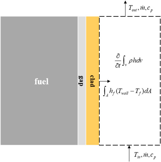
FIGURE 1. A simplified lumped coolant model.

In a steady-state condition, the energy balance equation is as follows:

$\dot{m}{c}_p\left(T_{out}-T_{in}\right)=\dot{Q},(42)$

and the outlet coolant temperature is simply obtained as

$T_{out}=T_{in}+\frac{\dot{Q}}{\dot{m}{c}_p},(43)$

where $\dot{m}$ is the coolant mass flow rate, $c_p$ is the specific heat capacity of the coolant, $h$ is the coolant enthalpy, $T_{wall}$ is the cladding wall temperature, $T_f$ is the coolant bulk temperature, and $\dot{Q}$ is the thermal power of the fuel element. The average coolant temperature is defined as an average of the inlet and outlet coolant temperatures:

$T_f=\frac{1}{2}\left(T_{out}+T_{in}\right).(44)$

For a time-dependent problem, the energy balance equation for the given control volume includes an additional time derivative term:

$\frac{\partial }{\partial t}{\displaystyle {\int }_v\rho hdv}=\frac{\partial }{\partial t}\left(\rho hV\right)=\dot{m}\left(h_{in}-h_{out}\right)+\dot{Q}.(45)$

Assuming a constant mass flow rate and the total mass is also constant as $\rho V=M$, the time derivative of the control volume’s enthalpy is

$\frac{\partial }{\partial t}\left(\rho hV\right)=\rho V\frac{\partial h}{\partial t}=\rho V\frac{\partial h}{\partial T}\frac{\partial T_f}{\partial t}=\rho V{c}_p\frac{\partial T_f}{\partial t},(46)$

where $c_p\equiv \frac{\partial h}{\partial T_f}$.

Applying Eq. 46 to Eq. 45, the time-dependent heat balance equation becomes

$M{c}_p\frac{\partial T}{\partial t}=\dot{m}{c}_p\left(T_{in}-T_{out}\right)+h_{f}A\left(T_{wall}-T_f\right).(47)$

To numerically solve the equation, we may apply the implicit Euler scheme:

$M{c}_p\frac{T_f^{\left(\ell \right)}-T_f^{\left(\ell -1\right)}}{\mathrm{\Delta }t}=\dot{m}{c}_p\left(T_{in}-T_{out}\right)+h_{f}A\left(T_{wall}-T_f^{\left(\ell \right)}\right).(48)$

The coolant temperature at the current time step is then expressed as follows:

$T^{\left(\ell \right)}=\frac{\frac{M{c}_p}{\mathrm{\Delta }t}{T}^{\left(\ell -1\right)}+2\dot{m}{c}_p{T}_{in}+h_{f}A{T}_{wall}}{\left(\frac{M{c}_p}{\mathrm{\Delta }t}+2\dot{m}{c}_p+h_{f}A\right)}.(49)$

2.4 Coupled Analysis Framework

The data exchange between the neutronics and the thermal-hydraulics part in the iMC code does not require an additional file exchange protocol since each calculation module is implemented in a single platform. The neutron transport simulation generates a user-specified thermal power distribution which is to be used in the heat transfer calculation. The thermal-hydraulics module performs the heat transfer analysis to provide the temperature evolution through the time step for the next time step neutron transport simulation.

Before the onset of the transient simulation, the system is needed to be in a steady state. The reactor system is first assumed to have a nominal constant temperature, and a steady-state neutron transport simulation calculates the local power distribution and global reactivity based on the arbitrary system condition. Using the neutronics output, a subsequent steady-state thermal-hydraulics simulation determines the corresponding temperature of all materials of interest. The temperature is then used in the next neutron transport simulation. Through this steady-state coupled iteration, material temperatures on a pin-by-pin basis are determined with the steady-state reactor power distribution.

Once the steady condition of the given reactor system is found, the transient simulation is commenced. Just like in the previous steady-state condition search iteration, the neutronics and the thermal-hydraulics coupled analysis is performed in every time bin, except the simulation schemes are based on the time-dependent formulation. The overall calculation flow of the coupled analysis is described in Figure 2.

FIGURE 2

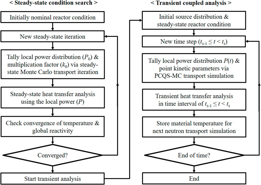
FIGURE 2. Flowchart of coupled analysis framework.

3 Numerical Results

3.1 CSBA-Loaded Fuel Assembly

For a preliminary study on the multi-physics feedback transient analysis, a CSBA-loaded fuel assembly is designed. In this model, a 17-by-17 PWR fuel assembly is composed of CSBA-loaded fuel pellets in place of the conventional plain UO₂ fuel. Also, four control rods are initially inserted into the fuel assembly as a means to impose a reactivity transient. A discretized single CSBA pellet model and the CSBA-loaded assembly are illustrated in Figure 3. The mesh was generated from Gmsh (Geuzaine and Remacle, 2009) software for the finite element heat transfer analysis. Detailed information about the CSBA model is presented in the study by Kim and Kim (2021b).

FIGURE 3

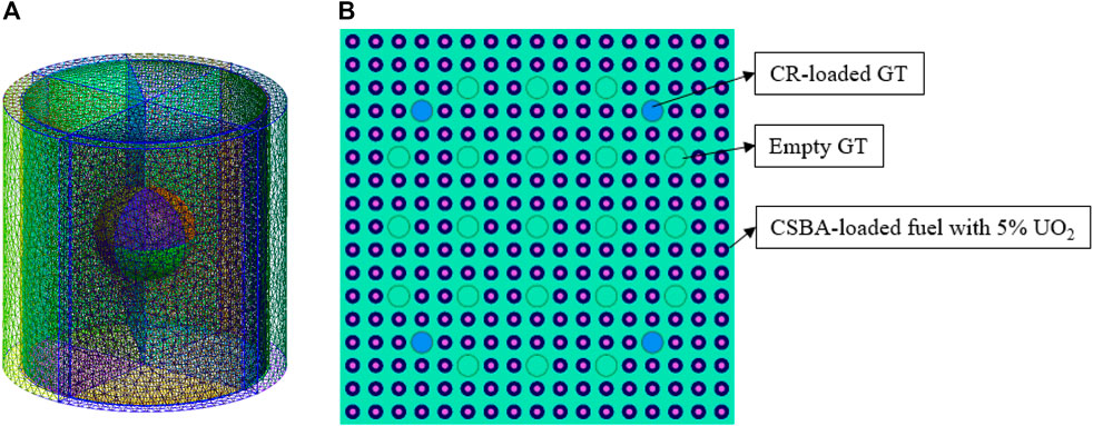
FIGURE 3. CSBA 3-D model (A) and CSBA-loaded fuel assembly with four control rods inserted (B).

To simplify the problem, a single layer of CSBA-inserted fuel is considered and the assembly is considered to be subjected to all reflective boundary conditions in four radial sides, top, and bottom. In the iMC, a user can provide reactivity transient scenarios in two different ways: changing material cross section by mixing or replacing with predefined materials or deforming the geometry by tuning surface parameters. In either case, the time-dependent parameter values are given in a user-defined function of time. To simulate the control rod withdrawal transient in this problem, we linearly mixed the coolant with the control rod material instead of geometric movement. The time-dependent mixing ratio is given in terms of volume fraction, and the corresponding new density is calculated in the iMC.

Before the transient simulation, a series of feedback iterations is performed to find an initial steady-state reactor system with the initial thermal power of 36 W/gU. The initial intra-pin temperature distribution and coolant average temperature are set as a constant value for the first steady-state transport simulation. With the obtained power distribution, the detailed temperature is updated. The iteration quickly converged to a steady-state after 2–3 iterations. The obtained pin-power distribution and pin average fuel temperature distribution are shown in Figure 4. The CSBA model used in this simulation is described in Table 1, and material properties used in the analysis are identical to those in the study by Kim and Kim (2020).

FIGURE 4

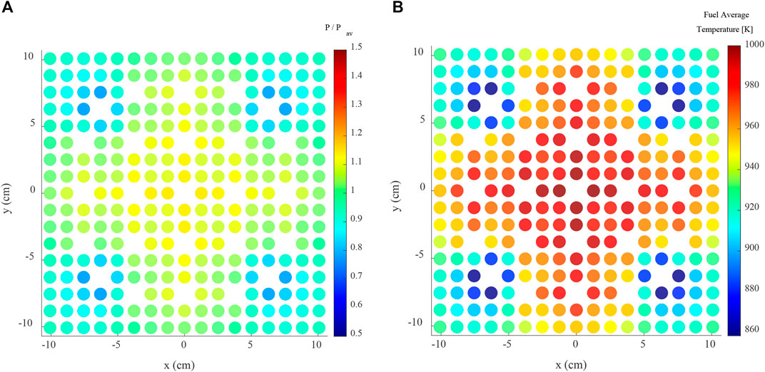
FIGURE 4. Initial steady-state pin-power distribution (A) and fuel temperature distribution (B).

TABLE 1

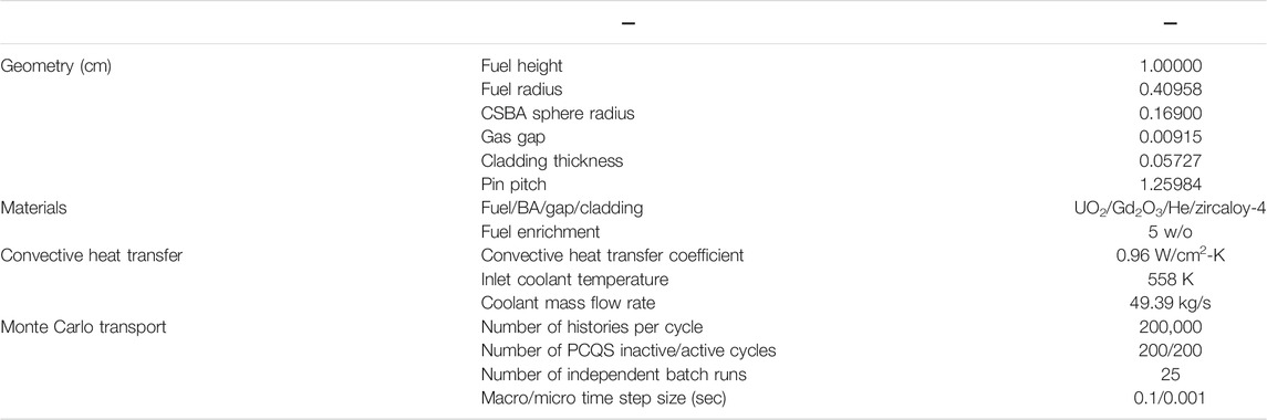
TABLE 1. CSBA fuel pellet analysis condition.

Starting from the initial material temperature and coolant density, the PCQS-assisted Monte Carlo transient calculation is done. The control rod material is linearly mixed with water from 0.5 to 1.5 s up to 20% of water volume fraction; 25 independent batch runs were performed to evaluate the uncertainty of the simulation. The reactor thermal power profile over the transient is shown in Figure 5. Without adequate temperature feedback from fuel, burnable absorber, and coolant, the reactor power increases exponentially with the given positive reactivity as the dashed line in Figure 5. However, the negative feedback effects of fuel and moderator temperatures suppressed the power excursion right after the end of additional reactivity insertion; the reactor power started to converge toward another stable state.

FIGURE 5

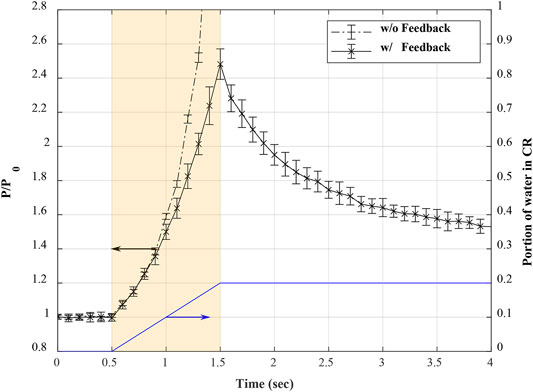
FIGURE 5. Time-dependent reactor power without feedback (dashed line) and with feedback (solid line) under a given portion of water mixed with control rods (blue line).

Figure 6 presents the fuel and moderator average temperature evolution with respect to the given thermal power transient. The fuel temperature response is rather prompt, although there is a slight lag to reach a stable state. This lag is largely due to the thermal inertia of the fuel and the heat dissipation delay from the fuel to the coolant. The coolant temperature response was clearly slower than that of the fuel since it is the last material of the heat transfer process. These temperature responses are also shown in local power and temperature in Figures 7, 8. The peak pin-power occurred at 1.5 s and decreased afterward, while the pin-wise fuel temperature monotonically increases to reach a plateau.

FIGURE 6

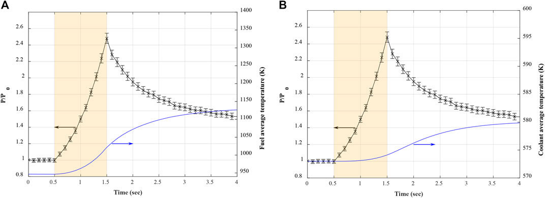
FIGURE 6. Time-dependent fuel average temperature (A) and coolant average temperature (B).

FIGURE 7

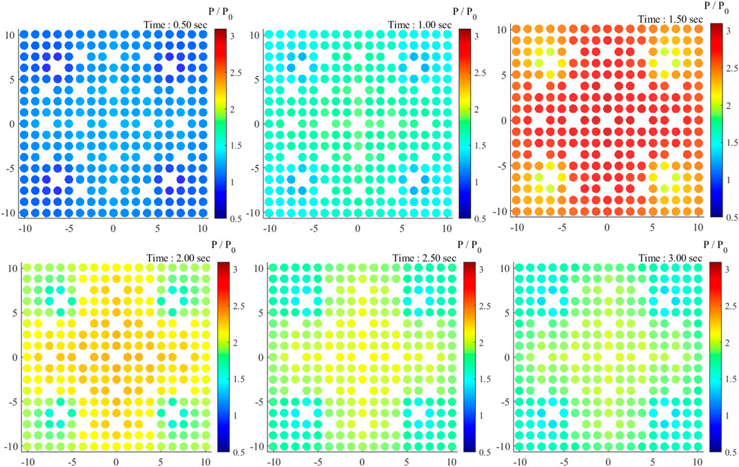
FIGURE 7. Time-dependent pin-power distribution from 0.5 to 3 s.

FIGURE 8

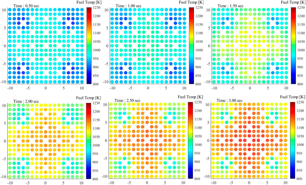
FIGURE 8. Time-dependent fuel temperature distribution from 0.5 to 3 s.

Table 2 shows the computation burden for major functions in a fraction of total computation time. The particle transport occupies most of the resources in the multi-physics simulation. The source list setting and combing takes less than 1% of the total burden, and the PK equation solving time is negligible. The FEM heat transfer calculation for each fuel pin is rather significant, implying a possibility of acceleration and algorithmic improvement for the matrix operation for larger problems.

TABLE 2

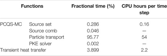
TABLE 2. Computation burden for major functions.

3.2 PWR Mini-Core Problem

This numerical study is for the verification of the iMC multi-physics coupled transient analysis framework. The only currently available Monte Carlo coupled analysis result is provided by the Serpent/SUBCHANFLOW framework. The TMI-1 mini-core problem provided in Ref (Ivanov et al., 2013) is considered for the iMC analysis, and the results are compared against the Serpent/SUBCHANFLOW analysis result presented in Refs. (Ferraro et al., 2019) and (Ferraro et al., 2020a). The TMI-1 mini-core problem consists of 15-by-15 PWR fuel assemblies in a 3-by-3 configuration as shown in Figure 9. In the center fuel assembly, 16 Ag-In-Cd control rods are initially fully inserted.

FIGURE 9

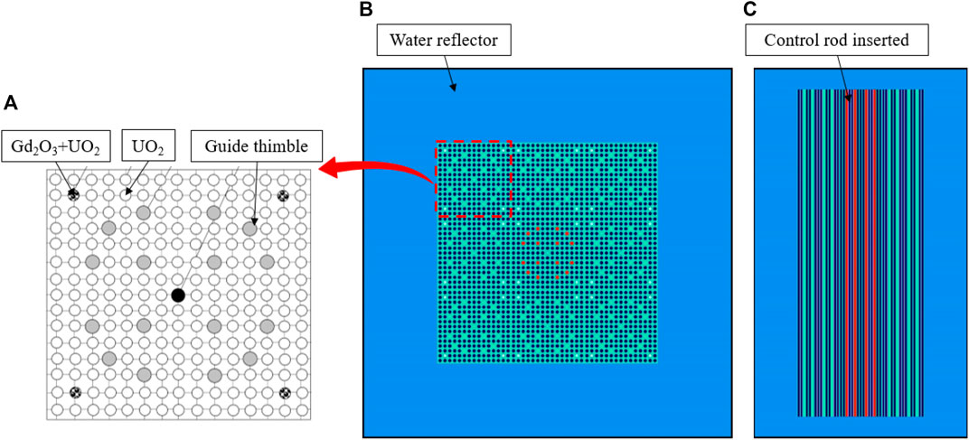
FIGURE 9. TMI-1 mini-core fuel assembly (A), x–y cut (B), and x–z cut (C) (not to scale).

The coolant contains soluble boron to make the system critical. The critical boron concentration (CBC) depends on the thermal-hydraulic model since the temperature and grid structure of the coolant channel are directly related to the borated coolant density. In the study by Ferraro et al. (2019), Serpent 2 and Tripoli-4 used a point-wise coolant model and neglected time delay in heat transfer from the fuel to the coolant, and the iMC obtained a similar value as in Table 3. When the coolant model is based on the detailed subchannel analysis code, the CBC value is lowered by about 200 ppm from the simple model due to the aforementioned reason.

TABLE 3

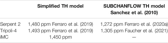
TABLE 3. Critical boron concentrations from different conditions and codes.

The simplified TH model in Ref. (Ferraro et al., 2019) assumes no thermal inertia of the fuel element, exhibiting no time delay of heat deposition inside the fuel by neglecting the time derivative term of the transient heat transfer equation. Since the iMC considers time-dependent heat transfer inside the fuel element without any approximation (but point model for the coolant), comparing the iMC analysis result with the simplified fuel heat transfer model is not adequate. Instead, we proposed to compare with the Serpent/SUBCHANFLOW coupled analysis model while the amount of static reactivity insertion is set to be identical. The static reactivity inserted in the Serpent/SUBCHANFLOW analysis is 354 pcm, with control rods withdrawn by 30 cm. We evaluated the equivalent control rod withdrawal length in the iMC that provides a similar static reactivity (Table 4). The critical boron concentration of the iMC model is determined on a trial basis iteration.

TABLE 4

TABLE 4. Control rod assembly withdrawal speed for Serpent 2 and iMC.

The reactor transient starts from 0.2 s by pulling out the 16 control rods from the active core with a constant speed pre-calculated in Table 4 for 1 s. The reactor is axially divided into 10 meshes for the fuel temperature modeling to follow the fuel temperature evaluation model in the SUBCHANFLOW analysis. In this calculation, the iMC used a volume-averaged temperature of each material in a single TH mesh as in the Serpent analysis. The simulation used 0.1 M histories per cycle, 200 PCQS inactive/active cycles, and 15 independent batch runs were performed for the evaluation of the uncertainties. The comparison of the calculated thermal power transient from the two codes and required computation time are presented in Figure 10 and Table 5, respectively.

FIGURE 10

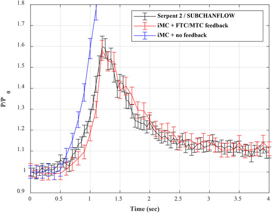
FIGURE 10. Comparison of Serpent/SUBCHANFLOW and iMC multi-physics using TMI-1 mini-core problem.

TABLE 5

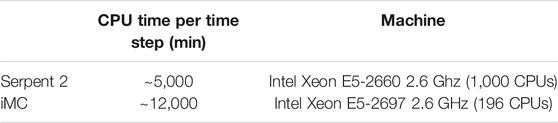
TABLE 5. Calculation time and condition for the TMI-1 mini-core problem.

As shown in Figure 10, without the negative temperature feedback of the reactor system, the thermal power exhibited an exponential excursion with the positive reactivity insertion. The iMC and Serpent simulation agreed well with each other except for the power evolution in response to the initial control rod withdrawal. This is because the control rod differential worth is slightly different in the two cases, albeit identical total reactivity insertion. Since the differential control rod reactivity worth becomes more significant as it approaches the active core center, the power growth is steeper in the iMC model as the withdrawal length is longer. The total reactivity insertion was similar in both cases (not exactly the same due to temperature difference), so the peak thermal power is evaluated to be very similar in the two codes. Figure 11 illustrates the local power transient of the mini-core problem. After 0.2 s of stable null transient, the control rod assembly is withdrawn from the bottom of the core for 1 s at a constant speed and stopped afterward. The axial power peak shifts toward the bottom of the core, and the local power transient behavior well agrees with the point reactor power result. Meanwhile, the time-dependent fuel pin temperature shown in Figure 12 monotonically increases during the period of the entire transient similar to the CSBA-loaded fuel assembly study. Also, the temperature peak skews toward the bottom of the core as the upward withdrawal of the control rod bank induces more bottom-skewed axial power profile.

FIGURE 11

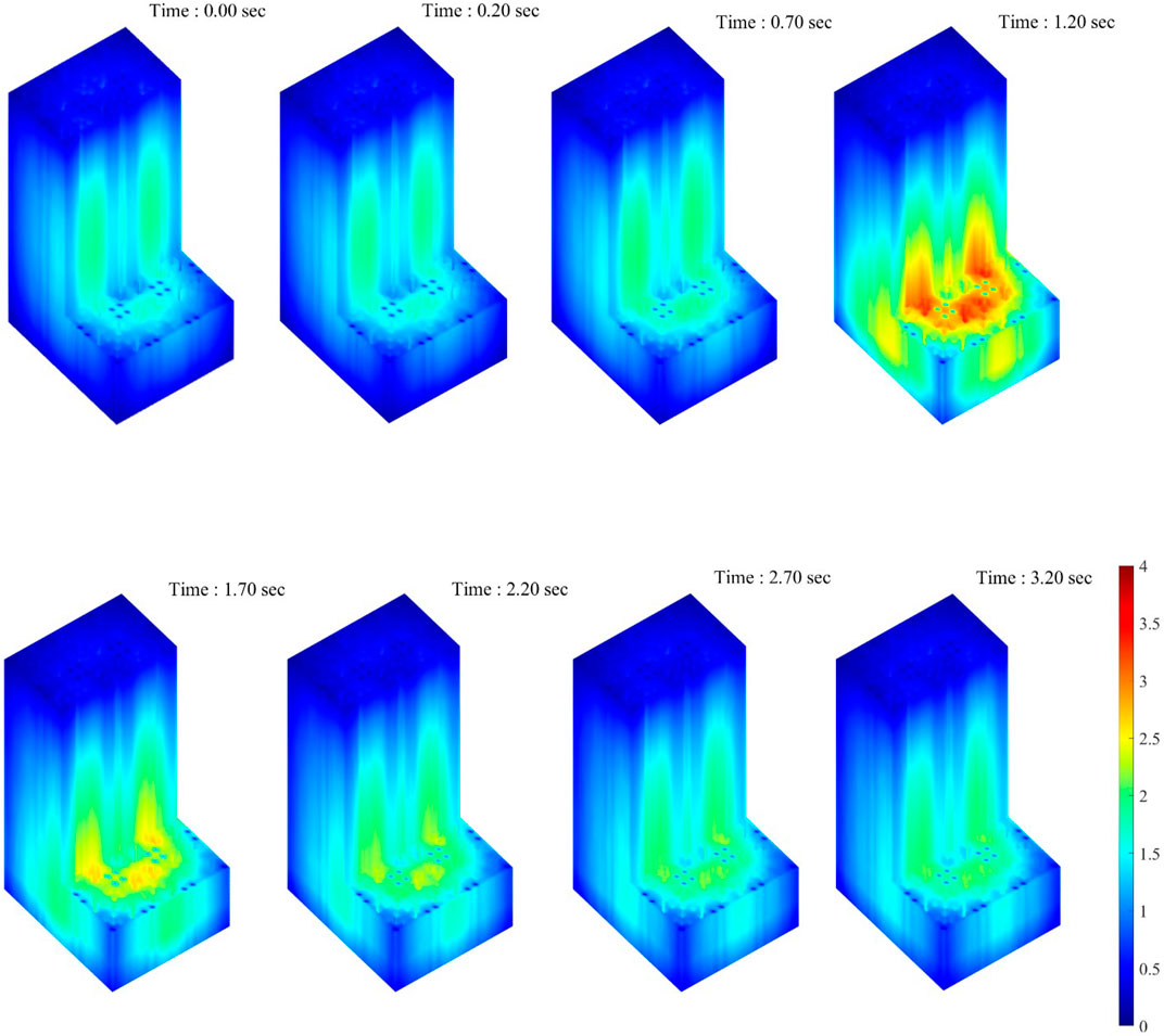
FIGURE 11. Transient pin-power distribution of the mini-core problem.

FIGURE 12

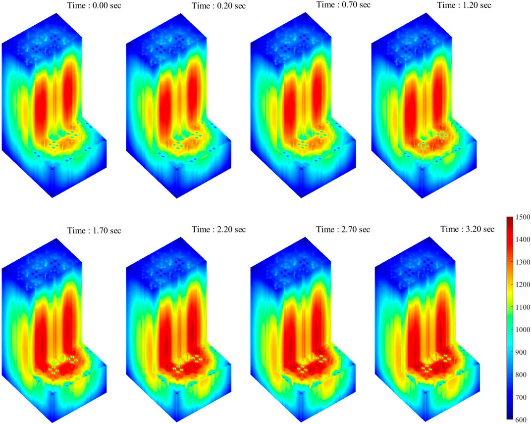
FIGURE 12. Transient fuel pin temperature distribution of the mini-core problem.

The computation time required for the simulation is relatively large compared to the steady-state simulation even for the Serpent. The Serpent Monte Carlo transport simulation is based on the dynamic Monte Carlo method, so the computation time is less affected by the time step size. Although the two analyses were performed in different calculation conditions, the iMC transport simulation time is still much longer than that of the Serpent using a longer macro time step size. However, this performance gap can be reduced by adopting the coarse-mesh acceleration methods to reduce inactive cycles and the ray-tracing improvement of the iMC transport function itself. Future effort on algorithmic enhancement is needed for such a demanding process along with a sufficient amount of computation resources for practical use of the Monte Carlo transient analysis.

4 Conclusion

In this work, we presented a multi-physics framework implemented in the iMC. The PCQS-MC-based transient neutron transport simulation and the finite element heat transfer are solved in a coupled framework to account for the temperature feedback effects in the time domain. The multi-physics framework is tested for a CSBA-loaded PWR fuel assembly when external reactivity is inserted via control rod removal from the system. The feedback correction of material cross-sections with adjusted temperature and density suppressed the additional reactivity and led the system to a stable state. The temperature responses of the system showed a slight lag from the initial perturbation due to the heat transfer delay, resulting in the power overshoot before the stabilization. The iMC multi-physics framework was also compared with the Serpent/SUBCHANFLOW coupled analysis framework on the TMI-1 mini-core problem for verification. The calculated time-dependent power evolutions from the two codes matched well, except for a minor discrepancy in the initial reactivity insertion period due to the different differential worth of the control rod.

The iMC analysis framework is especially useful for the 3-D complex fuel element as it can utilize the Gmsh-generated unstructured mesh grid for spatial discretization. For a more realistic reactor system simulation, the iMC multi-physics framework will adopt a subchannel analysis program in the near future. As we have demonstrated, such detailed analysis is essential for the accurate safety analysis of various fuel designs. We expect the applicability of the iMC multi-physics feature can be far extended for advanced PWR fuel elements that are continuously being developed and even for the molten salt reactor analysis.

Data Availability Statement

The raw data supporting the conclusion of this article will be made available by the authors, without undue reservation.

Author Contributions

HK developed the program and carried out the result under the supervision of YK.

Funding

This work was supported by the National Research Foundation of Korea Grant funded by the Korean government (NRF-2016R1A5A1013919) and BK21 FOUR (Fostering Outstanding Universities for Research) Project NO. 4120200313637.

Conflict of Interest

The authors declare that the research was conducted in the absence of any commercial or financial relationships that could be construed as a potential conflict of interest.

Publisher’s Note

All claims expressed in this article are solely those of the authors and do not necessarily represent those of their affiliated organizations, or those of the publisher, the editors, and the reviewers. Any product that may be evaluated in this article, or claim that may be made by its manufacturer, is not guaranteed or endorsed by the publisher.

References

Cherezov, A., Park, J., Kim, H., Choe, J., and Lee, D. (2020). A Multi-Physics Adaptive Time Step Coupling Algorithm for Light-Water Reactor Core Transient and Accident Simulation. Energies 13 (23), 6374. doi:10.3390/en13236374

CrossRef Full Text | Google Scholar

Faucher, M., Mancusi, D., and Zoia, A. (2021). Multi-physics Transient Simulations with TRIPOLI-4. EPJ Web of Conferences 247, 7019. doi:10.1051/epjconf/202124707019

CrossRef Full Text | Google Scholar

Ferraro, D., Faucher, M., Mancusi, D., and Zoia, A. (2019). “Serpent and TRIPOLI-4® Transient Calculations Comparisons for Several Reactivity Insertion Scenarios in a 3D PWR Minicore Benchmark,” in International Conference on Mathematics and Computational Methods applied to Nuclear Science and Engineering, Portland, Oregon, USA, August 25–29, 2019, 1734–1743.

Google Scholar

Ferraro, D., García, M., Valtavirta, V., Imke, U., Tuominen, R., Leppänen, J., et al. (2020). Serpent/SUBCHANFLOW Pin-By-Pin Coupled Transient Calculations for a PWR Minicore. Ann. Nucl. Energ. 137, 107090. doi:10.1016/j.anucene.2019.107090

CrossRef Full Text | Google Scholar

Ferraro, D., García, M., Valtavirta, V., Imke, U., Tuominen, R., Leppänen, J., et al. (2020). Serpent/SUBCHANFLOW Pin-By-Pin Coupled Transient Calculations for the SPERT-IIIE Hot Full Power Tests. Ann. Nucl. Energ. 142, 107387. doi:10.1016/j.anucene.2020.107387

CrossRef Full Text | Google Scholar

Ferraro, D., Valtavirta, V., García, M., Imke, U., Tuominen, R., Leppänen, J., et al. (2020). OECD/NRC PWR MOX/UO2 Core Transient Benchmark Pin-By-Pin Solutions Using Serpent/SUBCHANFLOW. Ann. Nucl. Energ. 147, 107745. doi:10.1016/j.anucene.2020.107745

CrossRef Full Text | Google Scholar

Ferraro, M., Valtavirta, V., Tuominen, R., Imke, U., Leppänen, J., and Sanchez-Espinoza, V. (2020). Serpent2-SUBCHANFLOW Pin-By-Pin Modelling Capabilities for VVER Geometries. Ann. Nucl. Energ. 135, 106955. doi:10.1016/j.anucene.2019.106955

CrossRef Full Text | Google Scholar

Fiorina, C., Clifford, I., Aufiero, M., and Mikityuk, K. (2015). GeN-Foam: a Novel OpenFOAM Based Multi-Physics Solver for 2D/3D Transient Analysis of Nuclear Reactors. Nucl. Eng. Des. 294, 24–37. doi:10.1016/j.nucengdes.2015.05.035

CrossRef Full Text | Google Scholar

Geuzaine, C., and Remacle, J.-F. (2009). Gmsh: A 3-D Finite Element Mesh Generator with Built-In Pre- and post-processing Facilities. Int. J. Numer. Meth. Engng. 79 (11), 1309–1331. doi:10.1002/nme.2579

CrossRef Full Text | Google Scholar

Guo, X., Shang, X., Song, J., Shi, G., Huang, S., and Wang, K. (2021). Kinetic Methods in Monte Carlo Code RMC and its Implementation to C5G7-TD Benchmark. Ann. Nucl. Energ. 151, 107864. doi:10.1016/j.anucene.2020.107864

CrossRef Full Text | Google Scholar

Ivanov, K., Avramova, M., Kamerow, S., Kodeli, I., Sartori, E., Ivanov, E., et al. (2013). Benchmarks for Uncertainty Analysis in Modelling (UAM) for the Design, Operation and Safety Analysis of LWRs-Volume I: Specification and Support Data for Neutronics Cases (Phase I). Organisation for Economic Co-Operation and Development.

Google Scholar

Jo, Y., Cho, B., and Cho, N. Z. (2016). Nuclear Reactor Transient Analysis by Continuous-Energy Monte Carlo Calculation Based on Predictor-Corrector Quasi-Static Method. Nucl. Sci. Eng. 183 (2), 229–246. doi:10.13182/nse15-100

CrossRef Full Text | Google Scholar

Kim, H. T. (2022). Study of Steady-State and Time-Dependent Monte Carlo Neutron Transport Coupled Multi-Physics Reactor Analysis in the iMC Code. Doctoral dissertation. Korea Advanced Institute of Science and Technology.

Google Scholar

Kim, H., and Kim, Y. (2021). Unstructured Mesh-Based Neutronics and Thermomechanics Coupled Steady-State Analysis on Advanced Three-Dimensional Fuel Elements with Monte Carlo Code iMC. Nucl. Sci. Eng. 195 (5), 464–477. doi:10.1080/00295639.2020.1839342

CrossRef Full Text | Google Scholar

Kim, H., and Kim, Y. (2020). Unstructured Mesh-Grid Multi-Physics Analysis with Monte Carlo iMC Code for Advanced Fuel Elements. Trans. Am. Nucl. Soc. 122 (1), 738–741. doi:10.13182/t122-32434

CrossRef Full Text | Google Scholar

Nguyen, X. H., Kim, C., and Kim, Y. (2019). An Advanced Core Design for a soluble-boron-free Small Modular Reactor ATOM with Centrally-Shielded Burnable Absorber. Nucl. Eng. Techn. 51 (2), 369–376. doi:10.1016/j.net.2018.10.016

CrossRef Full Text | Google Scholar

Park, I. K., Lee, J. R., Choi, Y. H., and Kang, D. H. (2020). A Multi-Scale and Multi-Physics Approach to Main Steam Line Break Accidents Using Coupled MASTER/CUPID/MARS Code. Ann. Nucl. Energ. 135, 106972. doi:10.1016/j.anucene.2019.106972

CrossRef Full Text | Google Scholar

Reed, W. H., and Hansen, K. F. (1970). Alternating Direction Methods for the Reactor Kinetics Equations. Nucl. Sci. Eng. 41 (3), 431–442. doi:10.13182/nse41-431

CrossRef Full Text | Google Scholar

Reed, W. H., and Hansen, K. F. (1969). Finite Difference Techniques for the Solution of the Reactor Kinetics Equations Massachusetts Inst. Of Tech. Cambridge: Dept. of Nuclear Engineering. doi:10.2172/4782171

CrossRef Full Text | Google Scholar

Sanchez, V., Imke, U., Ivanov, A., and Gomez, R. (2010). SUBCHANFLOW: A thermal Hydraulic Sub-channel Program to Analyse Fuel Rod Bundles and Reactor Cores. Cancun, Mexico: 17th Pacific Basin Nuclear Conference.

Google Scholar

Wang, Y., Schunert, S., Ortensi, J., Laboure, V., DeHart, M., Prince, Z., et al. (2021). Rattlesnake: A MOOSE-Based Multiphysics Multischeme Radiation Transport Application. Nucl. Techn. 207 (7), 1047–1072. doi:10.1080/00295450.2020.1843348

CrossRef Full Text | Google Scholar