 Ashfaq Ahmad1†
 Kinza Qadeer2†
 Ahmad Naquash2Fahid Riaz3Mudassir Hasan4
 Muhammad Abdul Qyyum5*
 Moonyong Lee2*
- 1Department of Computer Science, COMSATS University Islamabad (CUI), Lahore Campus, Lahore, Pakistan
- 2School of Chemical Engineering, Yeungnam University, Gyeongsan, South Korea
- 3Mechanical Engineering Department, Abu Dhabi University, Zayed City, United Arab Emirates
- 4Department of Chemical Engineering, College of Engineering, King Khalid University, Abha, Saudi Arabia
- 5Department of Petroleum & Chemical Engineering, Sultan Qaboos University, Muscat, Oman
Natural gas (NG) has been widely recognized as a cleaner fuel compared to other fossil fuels. Reserves of NG are typically located in remote areas, and their conditions and compositions vary geographically. The NG from such areas is transported in the form of liquefied natural gas (LNG). Liquefying NG is highly complex. Generally, the process is designed to be carried out under fixed natural gas (NG) conditions; hence, it may not perform well under variable NG conditions. Considering this issue, the use of an artificial intelligence approach, rather than the conventional optimization one, was investigated to make the LNG process feasible under variable NG conditions. This study is the first in this research area to train an artificial neural network (ANN) using the particle swarm optimization (PSO) algorithm as a learning method. The developed PSO-ANN model was used to predict the decision variables of a single mixed refrigerant (SMR) LNG process for its feasible design under varying NG conditions. The correctness of the predicted set of decision variables (NG conditions) was verified by inputting them into Aspen HYSYS. The output of the SMR-LNG process was the overall power at a constrained minimum internal temperature approach (MITA) value, i.e., 1.0 ≤ MITA ≤3.0. The prediction results of the PSO-ANN model were compared with those of the classical ANN backpropagation learning method. The success rate of the proposed PSO-ANN model was 80%. Furthermore, the proposed model can make the LNG process feasible for a diverse range of temperature and pressure values. A feasible process with a better MITA value can also be achieved by tuning the model parameters.
1 Introduction
Most natural gas (NG) reserves are located at remote and offshore sites. Generally, pipeline networks and/or cargo ships are used to transport NG to onshore sites and, consequently, into the trade market. For small distances (<2000 km), NG is transported in the gaseous form through pipeline networks. For long-distance transportation, liquefied NG (LNG) is preferred over gaseous NG mainly because of safety and economic factors (Qyyum et al., 2018a). Many offshore NG reserves have already been fully developed; their NG reserves are stored in the liquefied state to satisfy the global clean energy demand (Mohammad et al., 2021). Hence, new untapped NG reserves are entering the main trade loop also through the liquefaction approach (Xie et al., 2022). Figure 1 shows the growth trend of the LNG trade volume from 2005 to 2019 (Shell LNG outlook, 2019).
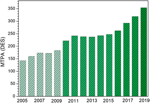
FIGURE 1. LNG trade volume trend from 2005 to 2019 (Shell LNG outlook, 2019).
However, liquefaction of NG is an energy-intensive and cryogenic-sensitive process. The high operating costs (40–60% (Qyyum et al., 2018c)) have a significant share in the total annualized costs (TAC) of LNG plants. The operating costs of LNG processes depend on many important design parameters, including pretreatment methods for raw NG feed (for LNG plant), NG composition, plant site ambient conditions, liquefaction technology (e.g., N2-expander, SMR, DMR, C3MR, MFC, etc.), and plant capacity (Khan et al., 2017; Qyyum et al., 2018c; He et al., 2018; Lee et al., 2018; Zhang et al., 2020). It has been found (Park et al., 2016) that the overall performance of LNG plants can be affected by variation in ambient temperature. Moreover, environmental relative humidity affects the performance of LNG plants that use air as a cooling medium, particularly in multistage compression units.
As LNG plants are initially designed at fixed values of design parameters by assuming a steady-state environment, there are abundant literature reports (Lee et al., 2002; Aspelund et al., 2010; Mokarizadeh Haghighi Shirazi and Mowla, 2010; Park et al., 2015; Xiong et al., 2016; Ali et al., 2018; He et al., 2019; Primabudi et al., 2019) on the analysis and performance improvement of LNG processes at fixed design parameters. Such parameters comprise primarily NG feed composition, pressure, and temperature. However, real-life LNG plants face many uncertainties in their design parameters that cannot be overlooked (Luu Trung Duong et al., 2018). Any uncertainty in the design parameters of LNG plants can affect the overall performance of the liquefaction process, which ultimately leads to an increase in the TAC. Although many possible uncertainties can be found in LNG processes, NG feed conditions (temperature and pressure) and composition are more likely to be prominent because of their reserve-to-reserve and ambient-to-ambient variations. Therefore, it is impossible to design a universal and robust LNG process to handle all types of NG feed under ambient conditions, and modifications in the process should be addressed depending on such variations, but the processes can be improved and/or maintained at their optimal execution by embedding the impacts of these uncertainties in the design parameters.
LNG processes with respect to the quantification uncertainty, sensitivity analysis, and robust optimization have been studied extensively. For instance, Cao et al. (2016) used Aspen Plus and a genetic algorithm (GA) to investigate the robustness of MR compositions for the single mixed refrigerant (SMR) process. They reduced the degrees of freedom in the variables to ensure the robustness of the MR and found strong robustness of the MR composition with 40% sustained energy efficiency, even though the ratio of the MR was restrained. Mortazavi et al. (2016) proposed a robust refrigerant mixture for the C3MR process by varying the NG feed compositions. They used Aspen HYSYS (v7.1) to simulate the C3MR process and then connected it to MATLAB (version 2010a) to demonstrate the gradient-assisted robust optimization. They found a robust MR under a 50% variation in the mass fractions of nitrogen, ethane, propane, i-butane, and n-butane. Wu et al. (2021) optimized the small-scale SMR LNG process and found that the energy consumption could be reduced by 29.8%. Furthermore, Ali et al. (2019) used a generalized polynomial chaos (GPC)-based surrogate modeling strategy to evaluate the reliability of GA- and particle swarm optimization (PSO)-optimized SMR processes under uncertain MR compositions with a 3% standard deviation from the mean of optimal values. They investigated six output objectives, that is, the liquid fraction of the LNG product, LNG temperature, MR liquid fraction at the inlet of the LNG heat exchanger, duty of the LNG exchanger, minimum internal temperature approach (MITA) inside the LNG cryogenic exchanger, and overall compression power. Most recently, (Qyyum et al., 2019) studied the impact of operational variables on the MITA inside warm MR heat exchangers, MITA inside cold MR heat exchangers, and the overall compression power of the DMR process. They presented an uncertainty quantification followed by a global sensitivity analysis at a fixed NG feed composition and conditions for the DMR liquefaction process. Moreover, they performed global sensitivity analysis by developing a surrogate model and then used a multiplicative dimension reduction method. To study the impacts of uncertain variables (warm MR composition, cold MR composition, suction and discharge pressures of warm MR, and cold MR loop) on MITA and the overall energy consumption, they used the well-known Monte Carlo and quasi-Monte Carlo approaches.
Based on the existing literature, several research groups have investigated and optimized LNG processes under constant NG composition and conditions. Uncertainty quantification and sensitivity analysis of the DMR process, which was performed at fixed NG composition and conditions, have been performed. Attempts have been made to find a robust MR composition under varying NG compositions, rather than NG conditions, using conventional robust optimization techniques. Notably, simultaneous changes in the NG composition and conditions are not mandatory and are not dependent on each other. Sometimes, the NG composition remains constant for a long time, but the NG conditions can vary and vice-versa. However, any changes in either the conditions or composition can result in the LNG plant violating the second law of thermodynamics, such as a negative MITA value inside an LNG cryogenic exchanger and/or an uneconomical cryogenic heat transfer operation with a MITA value of <1.0°C. Generally, LNG plants with a MITA value of 1.0–3.0°C are considered cost-effective and feasible (Hasan et al., 2009; Qadeer et al., 2018). Therefore, for any uncertain NG feed composition and/or condition, it is necessary to maintain the LNG process within the MITA value of 1.0–3.0°C.
This is the first study that enables the LNG processes to be carried out under uncertain NG pressure and temperature conditions using an artificial intelligence approach rather than the conventional optimization approaches. The krill-herd-based optimized SMR-LNG process presented by Qadeer et al. (2018) was adopted for the proposed study. The modified coordinate descent (MCD) algorithm was used to extract the training data on the SMR-LNG process under varying NG pressures and temperatures. Any algorithm can be used for data generation; however, the MCD algorithm was used because of its robustness and accuracy for SMR processes, as shown in this study. Similarly, PSO is a well-proven optimization algorithm; therefore, we used PSO for the artificial neural network (ANN) parameter optimization. However, any optimization algorithms can be used with an ANN to improve the results in the future. A back-propagation (BP)-based ANN prediction model was used. This BP-learned ANN was then trained in a cascaded manner on the SMR-LNG process training data obtained through the MCD approach. To evaluate the performance of the ANN model, uncertain NG conditions were introduced in the HYSYS-simulated SMR-LNG process by MATLAB (version 2019a). For any uncertain NG temperature and/or pressure within specified ranges, the ANN model quickly estimated the decision variables to make the LNG process, and the decision variables of the SMR-LNG process were estimated. This estimated set of decision variables was fed to the Aspen HYSYS simulator to make the SMR-LNG process feasible. The appropriateness of the predicted set of decision variables was verified by inputting them into the Aspen HYSYS simulator. The output of the SMR-LNG process was the overall power at a constrained MITA value, i.e., 1.0 ≤ MITA ≤3.0. The prediction results of the PSO-ANN model were compared with those of the classical ANN BP learning method.
2 Methods
The method adopted in this study is illustrated in Figure 2. First, the SMR-LNG process was simulated using Aspen HYSYS® v10. After the simulation, data were extracted by establishing a link between Aspen HYSYS® and MATLAB. The extracted data were then normalized for the robustness of the training algorithm. In the normalized database, the training and testing datasets consisted of 80 and 20% of the original data, respectively. The PSO-ANN model was developed and implemented by adopting a cascade training procedure for the datasets. After implementation, the performance of the developed model was evaluated using 15 test datasets.
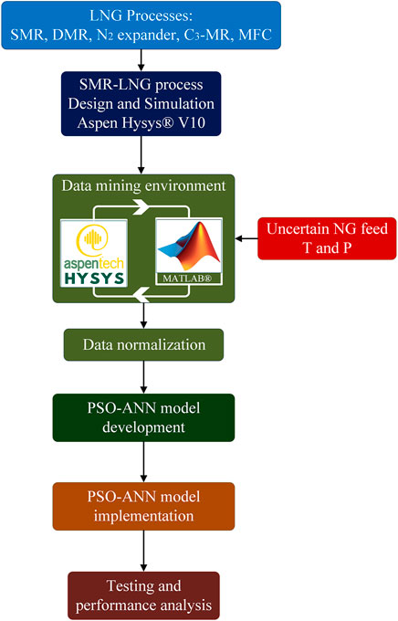
FIGURE 2. Research methodology of the proposed study.
2.1 Single Mixed Refrigerant–Liquefied Natural Gas Process: Simulation and Description
Among the LNG processes, the SMR process (also known as the poly-refrigerant integrated cycle operation (PRICO) process) is the simplest and most well-suited for small-scale and offshore applications, owing to its compactness, easy operability, and simple design (Qyyum et al., 2018b). Additionally, the SMR process requires less capital investment than other processes (Qyyum et al., 2018c). This process consists of a compression unit equipped with interstage coolers, a main cryogenic exchanger, and an expansion valve. A detailed description of the SMR-LNG process is presented in Section 2.2.
2.2 Process Description
The flow diagram of a typical SMR-LNG process is shown in Figure 3. The NG stream (NG) at 32°C and 50 bar enters CHX-1 and leaves as a 100% saturated liquid at –149.3°C. The stream 1 leaving CHX-1 is passed through JTV-1 for isenthalpic expansion to 1.209 bar. This expansion process produces LNG at –158.5°C with a 92% liquefaction rate, which then enters the phase separator (V-1) to separate LNG and ends flash gases (EFG). This liquefaction process is supported by the SMR cycle. The SMR cycle, comprising C1, C2, C3, and N2, is compressed to 69.45 bar in a series of compressors and interstage coolers. The function of the interstage coolers is to maintain the MR temperature at 40°C at the compressor inlet. After compression, condensation of the high-pressure MR occurred in the after-cooler (C-4) and CHX-1. This high-pressure condensed MR enters JTV-2 for isenthalpic expansion to 1.65 bar and then re-enters CHX-1 to deliver its cold energy for the condensation of both the NG and MR streams. The outlet SMR stream 15 leaves CHX-1 at 37°C and is recycled to complete the refrigeration loop.
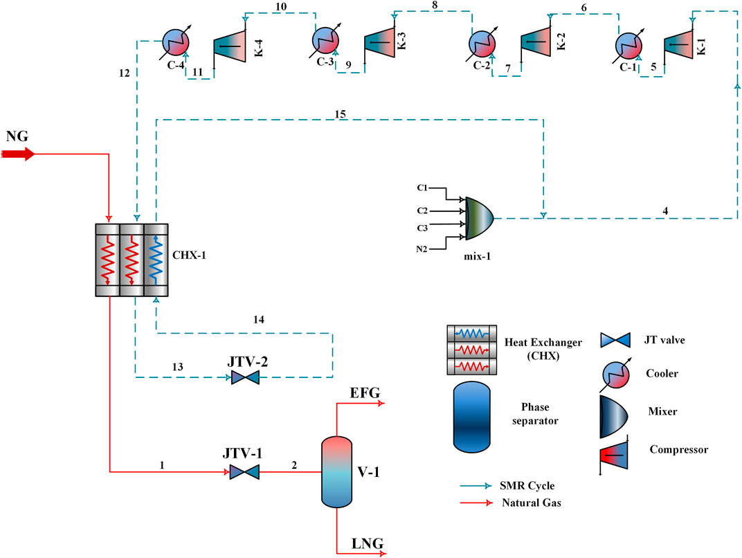
FIGURE 3. Schematic representation of the process flow diagram of the SMR-LNG process.
2.3 Process Simulation
The SMR-LNG process was simulated using the process simulation software application Aspen HYSYS® v 10. In Aspen HYSYS, the Peng–Robinson model (Peng and Robinson, 1976) was selected as an equation-of-state model to calculate the thermodynamic properties, whereas the Lee–Kesler (Kesler and Lee, 1975) model was adopted for enthalpy calculations of the refrigerant and LNG streams. The following assumptions were made for the SMR-LNG process simulation:
1) The heat loss to the surroundings is zero.
2) Water is used as a cooling medium in the interstage and after-coolers.
3) The outlet temperature of the process stream after the interstage and after the coolers was maintained at 40°C.
4) The efficiencies of the compressors are kept at 75%.
5) The pressure drops across CHX-1 on the hot and cold sides are 1.0 and 0.1 bar, respectively.
The design parameters and constraints of the process simulation, listed in Table 1, were obtained from Qadeer et al. (2018). The stream conditions for the simulated SMR-LNG process are listed in Table 2.

TABLE 1. Design parameters and constraints of the SMR-LNG process.
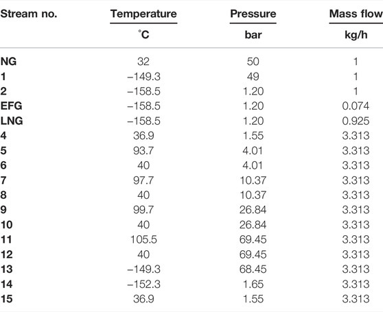
TABLE 2. Process stream conditions of the SMR-LNG process.
3 Data Collection
This study aimed to develop a particle swarm-assisted artificial neural network (PSO-ANN) model for the prediction of the design parameters of the SMR-LNG process for its feasible operation under given NG conditions. A comprehensive database of 1,000 data samples in terms of input decision variables and the overall output power with constraint (1.0 ≤ MITA ≤3.0) was collected using the Aspen HYSYS® v10 process simulator. The simulator was linked to the Visual Studio platform, and the database was extracted using the modified coordinate descent (MCD) method, as shown in Figure 4.
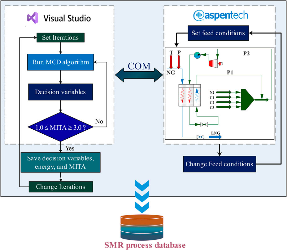
FIGURE 4. Aspen HYSYS–Visual Studio-based data mining environment.
Figure 4 shows that for a specific set of feed conditions, the decision variables of the SMR-LNG process vary in such a way that a feasible SMR-LNG process is obtained, i.e., the MITA value lies between 1.0 and 3.0. The MCD is terminated, and the values of decision variables, corresponding energies, and MITA values are saved in the database. This process was repeated by setting new iterations of MCD and adjusting a new set of feed conditions. Table 2 lists the feed conditions and other simulation assumptions that were used to build the data mining environment. Table 3 represents the upper and lower bounds of each decision variable within which the database was generated.

TABLE 3. Decision variables of the SMR process with their upper and lower bounds.
To establish the nature of the relationship among all feed conditions, decision variables, overall power, and MITA values within the collected database of the SMR-LNG process, the coefficient of determination (R2) was calculated, as given in Table 4. The coefficient of determination indicates that the percentage of the total variation in the dependent variable can be explained by the linear relationship between the dependent and independent variables. For example, 98.7% of the total variation in the overall power can be explained linearly with respect to C1, whereas the remaining 1.3% remains unexplained. Table 4 shows the moderate relationships among different variables, except for a few (in bold). This makes the feasibility of the SMR-LNG process a very complex problem for the user-defined set of feed conditions.
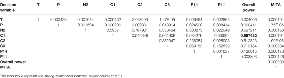
TABLE 4. Summary of SMR-LNG process parameters in terms of R.2.
4 Data Normalization
For the robust operation of any training algorithm, it is necessary that all the input and output parameters of a database are normalized in the same range (−1 to 1) (Yagiz and Gokceoglu, 2010; Armaghani et al., 2014; Amiri et al., 2016; Jahed Armaghani et al., 2016; Ghasemi, 2017). Thus, the database prepared in the previous section was normalized using Eq. 1:
where
4.1 Selection of Model Parameters
In the PSO-ANN model, several parameters were associated with both the ANN and PSO algorithms. ANN parameters that comprise ANN architecture include the number of hidden layers, neurons, training rule, training algorithm, and network type. The PSO parameters are swarm size (N), velocity coefficients (c1 and c2), and inertial weight (w). To obtain the optimum PSO-ANN model, the design parameters of both the PSO and ANN algorithms must be optimized.
4.1.1 Classification of Variables in the Single Mixed Refrigerant–Liquefied Natural Gas Process
First, the optimum ANN architecture was obtained by calculating the design parameters. For this purpose, the variables of the SMR-LNG process are first classified into independent and dependent variables. In our problem regarding feasible designs of the SMR-LNG process under varying feed conditions, 10 variables in the SMR-LNG process were considered. Table 5 presents the classification of these variables into independent and dependent variables.
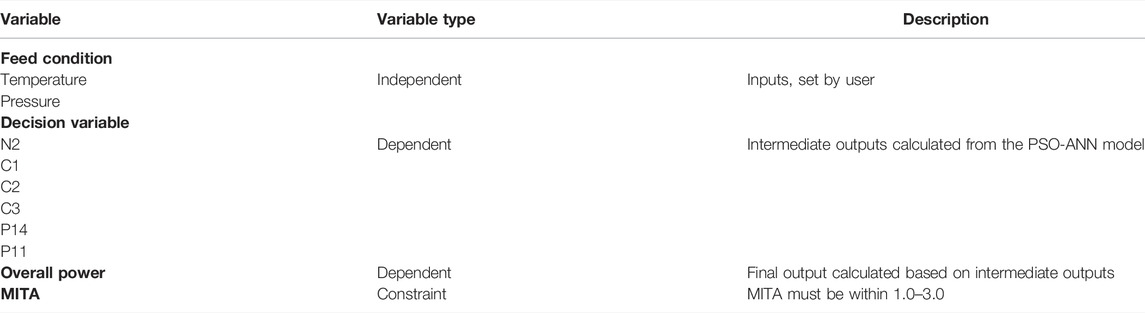
TABLE 5. Summary of SMR-LNG process variables.
4.1.2 Cascaded Training Procedure
In the SMR-LNG process, there are two feed conditions and six decision variables. These eight variables are fed into the SMR-LNG process to make it feasible. SMR-LNG is a very complex process, and it is difficult to determine any relationship between one variable and the others. One method is to predict each decision variable explicitly by training the model based on the feed conditions only. However, this may lead to incorrect results, owing to the existence of a nonlinear relationship among all decision variables. In this study, a cascaded training procedure is adopted. In this procedure, one decision variable is predicted based on the feed conditions, and then, the next decision variable is predicted based on the feed conditions and the already predicted variable.
One way to train the model is to explicitly predict every decision variable based on feed conditions. However, this may not make the SMR-LNG process feasible, owing to the existence of some relations among the six decision variables. Thus, in this cascaded ANN architecture, the number of nodes in the input layer varied from two to seven, whereas the number of neurons in the output layer remained constant. As the decision variable would be randomly predicted first, there are 480 possible permutations/settings for the two feed conditions and the six decision variables. One permutation of the variables, set as independent and dependent in the cascaded training procedure, is given in Table 6. In this study, the permutation of the variables given in Table 6 is performed. However, all permutations can be exploited to achieve the desired results.
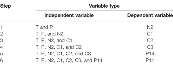
TABLE 6. Arrangement of input and output variables of cascaded ANN architecture.
4.1.3 Optimum Design Parameters of the Artificial Neural Network Architecture
Regardless of the permutation of variables, it is necessary to determine the design parameters of the cascaded ANN architecture. From all ANN parameters, the selection of the network type, training rule, and training algorithm are rigorously discussed in the literature (Hush 1989; Kanellopoulos and Wilkinson, 1997). Previous studies (Meulenkamp and Grima, 1999; Ornek et al., 2012; Ceryan et al., 2013) have found that among other training rules, the Levenberg–Marquardt (LM) algorithm is efficient in solving engineering problems. Furthermore, it has been proven that an ANN with one hidden layer is sufficient for solving all types of problems. In addition, the architecture of an ANN with only one hidden layer decreases the complexity of the model, resulting in a decrease in overfitting. The backpropagation training algorithm (which was later replaced with the PSO algorithm), along with the feed-forward network, was found to be a more efficient setup by many researchers (Hornik et al., 1989; Basheer, 2000; Hecht-Nielsen, 2018). The number of nodes in the hidden layer
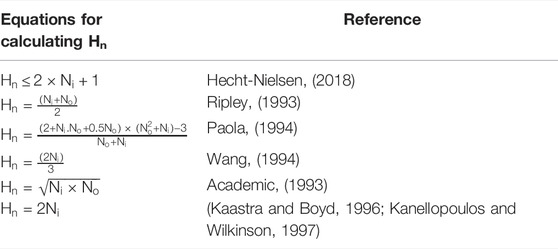
TABLE 7. Equations from the literature for the determination of
According to this table, the upper bound of
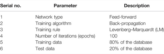
TABLE 8. ANN parameters set for calculating the number of nodes in the hidden layer (Hn).
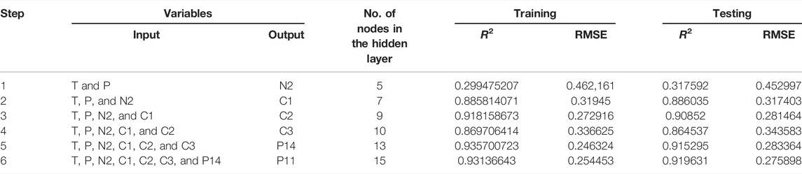
TABLE 9. Optimum value of Hn calculated for the cascaded ANN model given in Table 6.
4.1.4 Determination of the Particle Swarm Optimization Parameters
As mentioned earlier, the PSO algorithm was integrated with an ANN for the prediction of the decision variables for the feasible design of the SMR-LNG process under varying values of temperature and pressure (feed conditions). PSO accomplishes the task of minimizing the fitness/objective function by selecting the optimum values of the weights and biases. The objective function f that is considered to be optimized through PSO is the root mean square error (RMSE) of the ANN, which is given as follows:
where
There are four parameters that are associated with the PSO algorithm: velocity coefficients (c1 and c2), inertia weight (w), number of particles in the swarm (swarm size N), and number of iterations. The inertia weight is normally a random number between 0 and 1. Previous research has shown that the PSO parameters can be obtained by conducting sensitivity analyses. Mohamad et al. (2015) and Momeni et al. (2015) presented 12 combinations of c1 and c2 in the range of 0.8–3.2, such that the sum of c1 and c2 is 4. Alam et al. (2015) found the optimum range of velocity coefficients: c1 lies between 1 and 2.5, and c2 lies between 2 and 3. Furthermore, Hajihassani et al. (2014) and Momeni et al. (2015) suggested that the velocity coefficient values of c1 = c2 = 2 and inertia weight = 0.25 give optimum results. Thus, after the conclusion made on the previously reported research, the velocity coefficient of 2 and the inertia weight of 0.25 were used for all evaluations of the PSO-ANN model used in this study. The swarm size has a significant impact on the prediction performance of the PSO-ANN model, but there is no specific method to determine the swarm size, except for the well-known trial and error method. For the given cascaded training procedure, two permutations were selected from 480 permutations. For the first permutation, the RMSE values were selected for various numbers of particles in a swarm, and for the second permutation, the R2 value selected for various numbers of particles in a swarm are calculated, as shown in Figures 4, 5, respectively. From Figure 5, it is evident that while predicting N2, C1, C2, and C3, the minimum RMSE value is obtained at a swarm size of 10. Similarly, the swarm size was found to be 15 when predicting P14 and P11. Thus, unusual results were obtained, as shown in Figure 6. Swarm sizes of 15 (for the predictions of C1, C2, and C3) and 25 (for the predictions of N2, P14, and P11) were obtained. This implies that changing the permutation of variables leads to a change in the swarm size. Thus, determining the optimum swarm size for the proposed PSO-ANN model is not easy. However, as shown in Figures 5, 6, satisfactory predictions can be achieved for swarm sizes of less than 30. Thus, to prevent the model from being overburdened, all swarms with sizes smaller than 30 are exploited in the proposed study.
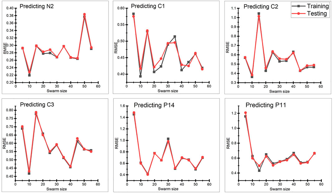
FIGURE 5. Calculation of optimum swarm sizes with respect to RMSE.
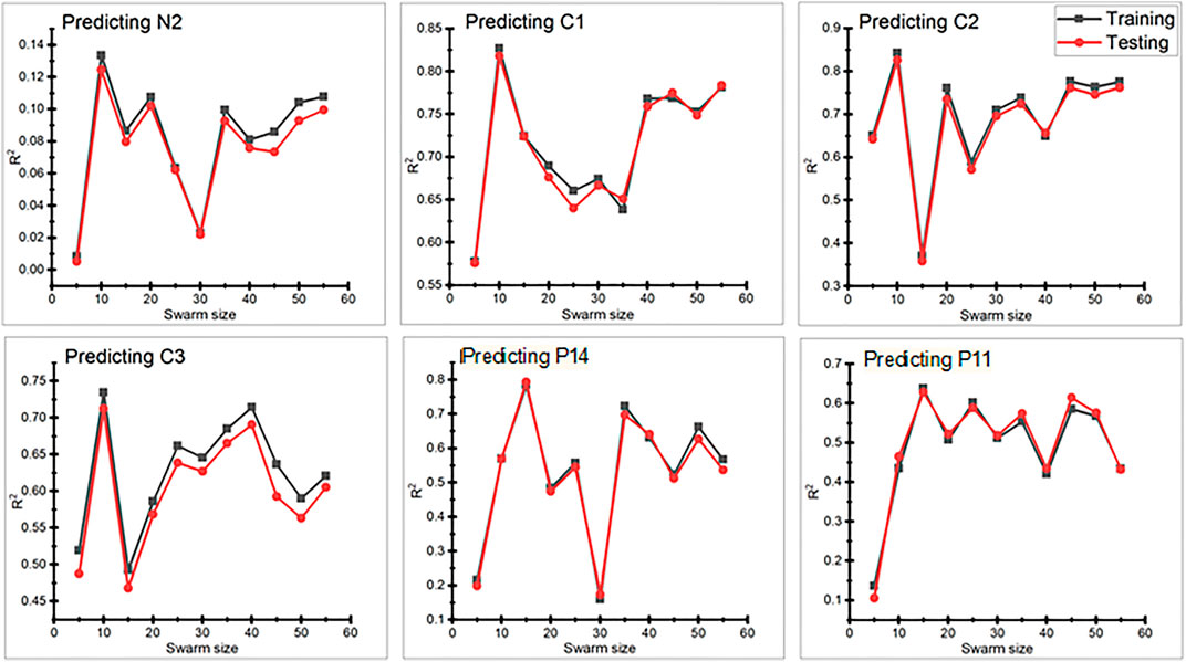
FIGURE 6. Calculation of optimum swarm sizes with respect to R2.
4.2 Optimum Particle Swarm Optimization–Artificial Neural Network Architecture
After data collection and normalization, data division, and calculation of the optimum parameters of both the ANN and PSO algorithms, the optimum PSO-based ANN model is achieved. A summary of all the parameters of the optimum PSO-ANN model is presented in Table 10.
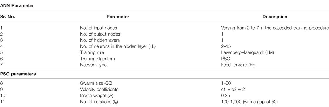
TABLE 10. Optimum PSO-ANN parameters for the design of the model.
5 Particle Swarm-Assisted Artificial Neural Network
An ANN consists of very complex interconnections of processing units called neurons. An ANN possesses three types of layers: one input layer, one output layer, and some hidden layers. Neurons are placed in the hidden and output layers, whereas the input layers consist of nodes that are equal to the number of independent variables. All nodes and neurons in the three types of layers are connected to each other. Each connection is associated with a weight, and each layer is associated with a bias. The values of these weights and biases are adjusted by the values of the input variables and their corresponding output variables to attain the minimum value of the error function. The basic ANN model is illustrated in Figure 7.
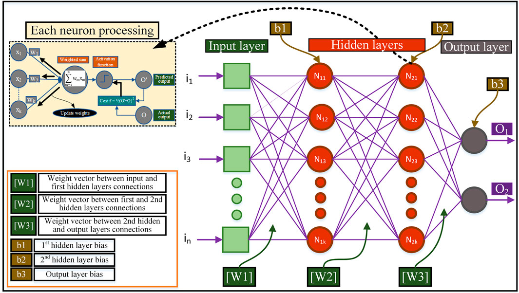
FIGURE 7. Basic artificial neural network architecture.
This model accepts n independent variables/features i1, i2 ... in and produces two outputs/dependent variables O1 and O2. [W1], [W2], and [W3] are the weight vectors, and b1, b2, and b3 are the biases associated with the connections and layers, respectively. For the simplest 1-1-1 neural network, if the number of independent variables is i = 1, 2, … n and the number of neurons in the hidden layer is j = 1, 2, … ,k, then Wij represents the weights of the connections between the ith input variable to the jth neuron in the hidden layers, and bj represents the bias coupled with the jth neuron in the hidden layer; Wj represents the weights of the connection between the jth neuron in the hidden layer and the single output layer’s neuron; b1 represents the bias coupled with the single neuron in the output layer. A total of k × (n + 2) + 1 parameters (weight plus bias) were used in the network (Rukhaiyar et al., 2018). After completing the structure of the ANN model, the training procedure was initiated on the training dataset, which consisted of known values of the input variables with their corresponding output values. The training dataset of the ANN network was used to find the optimal values of the weights and biases. Typically, backpropagation (BP), gradient descent, and Levenberg–Marquardt (LM) optimization algorithms are used to attain optimum values of weights and biases (Shahin et al., 2002). The training of one neuron using the BP method is shown in Figure 6 (enlarged part), where the weighted sum is calculated at the node. This weighted sum is then operated using an activation function to obtain the predicted output. Some common activation functions are listed in Table 11 (Karlik and Olgac, 2010).
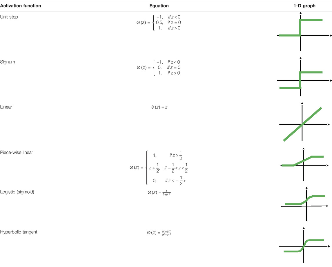
TABLE 11. Activation functions for the artificial neural network.
The predicted output and the actual output (as given in the training dataset) are compared, the cost function is calculated, and weights and biases are updated. This procedure is repeated until a minimized cost function is achieved. The same procedure was repeated for all neurons. Once the network is optimized, it is tested using unseen data. Because of its dependence on the selection of the initial point, the BP algorithm and other conventional methods become very susceptible to initial weights. Furthermore, these methods have fewer learning capabilities and are trapped at the local minimum point (Shahin et al., 2002). These limitations can be overcome by finding the optimal value using metaheuristic algorithms such as particle swarm optimization (PSO), ant colony optimization (ACO), genetic algorithm (GA), and differential evolution algorithm. Inspired by the social and cooperative behavior of bird flocks, PSO has been proven to be the most robust optimization technique. The prediction performance of the ANN improves when coupled with PSO (Panigrahi et al., 2011; Raja and Rajagopalan, 2014; Talal, 2014). In this study, a PSO-based ANN model was implemented to estimate the feasible values of all operating parameters of the SMR-LNG process at user-defined values of the feed conditions.
5.1 Particle Swarm Optimization–Artificial Neural Network Model Implementation
In the proposed study, the BP technique was replaced by the PSO algorithm to optimize the weights and biases for the optimum training of the ANN architecture. Optimum training of the ANN through PSO was performed in MATLAB (version R2019b). The implementation of the PSO-ANN model for the SMR-LNG process is described in the flowchart in Figure 8. All six decision variables of the SMR-LNG process were predicted using the user-defined test values of temperature (T) and pressure (P). A demonstrative example of the proposed PSO-ANN model to provide insight into the cascaded training and prediction mechanism is shown in Figure 9. The user-defined values of T and P were set as 20°C and 40 bar, respectively.
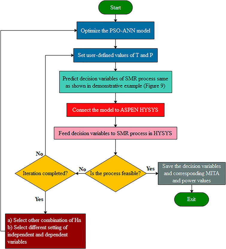
FIGURE 8. Framework of the proposed PSO-ANN model for the SMR process.

FIGURE 9. Demonstrative example of cascaded training and the prediction procedure of the PSO-ANN model.
6 Performance Evaluation
For the performance evaluation, 15 test datasets of the feed conditions were used. The PSO-ANN model was tested on these datasets, and its estimation performance was compared with that of the conventional BP-ANN model. For each set of test data, the SMR-LNG process was in an infeasible state (MITA <1). Thus, new values of all decision variables must be estimated for the feasible operation of the SMR-LNG process. Table 12 shows the prediction performance of the PSO-ANN model on the test datasets. It was concluded that the PSO-ANN model made the SMR-LNG process feasible for 12 out of 15 datasets by accurately estimating the decision variables. The success rate of the PSO-ANN model was 80%. Three cases of failure were observed. However, this 20% failure may be rectified by adapting other permutations of the variables in the cascaded training procedure. For a fair comparison, the estimation of decision variables was also made using the standard BP-ANN model (which does not use the PSO optimizer), as given in Table 13. It was found that the BP-ANN model predicted the decision variables accurately for only two out of the 15 test datasets; hence, the success rate was 13.33%. In the BP-ANN model, owing to its extrapolation behavior, the few predicted flow rates were negative, which is impossible in a real scenario.
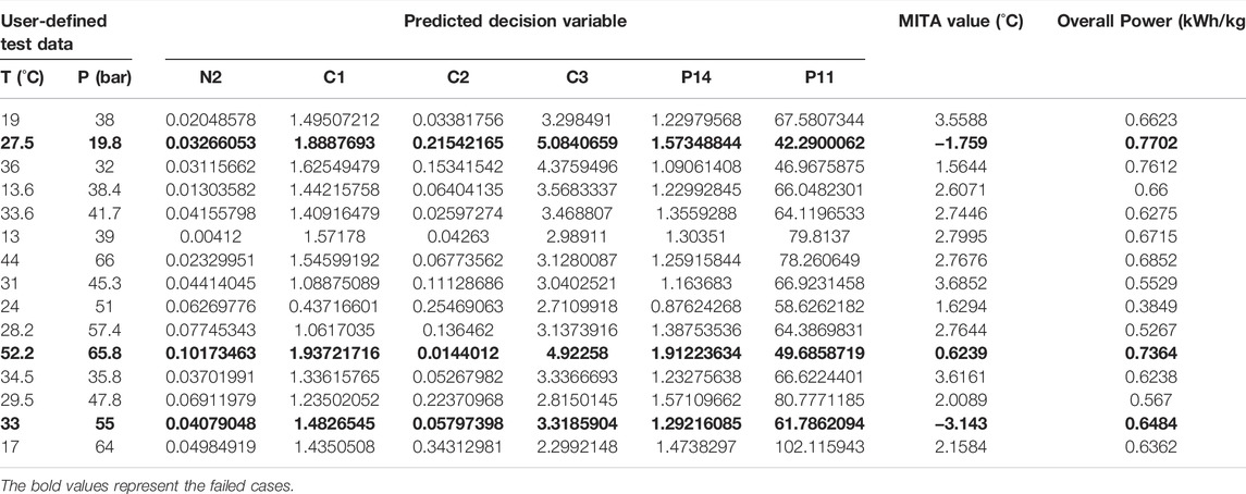
TABLE 12. PSO-ANN performance: estimated decision variables and their corresponding MITA and overall power values against user-defined test data.
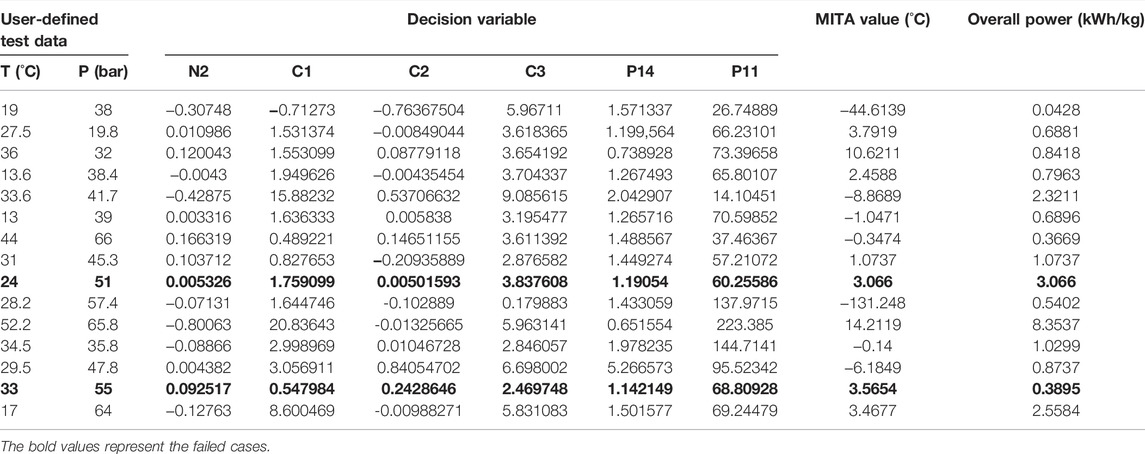
TABLE 13. BP-ANN performance: estimated decision variables and their corresponding MITA and overall power values against user-defined test data.
Figure 10 shows the relationships between different trained models and the output variables for the permutation of the variables given in Table 6. The coefficient of correlation (R) measures the degree of dependence between two quantities. Its value varies from −1 to 1. A higher value of R indicates a stronger relationship. Thus, it is clear from Figure 10 that the probability of prediction correctness is higher for C1 and C3, lower for N2, and medium for C2, P14, and P11. Furthermore, prediction accuracy can be improved by employing any other permutation in the cascaded training procedure.
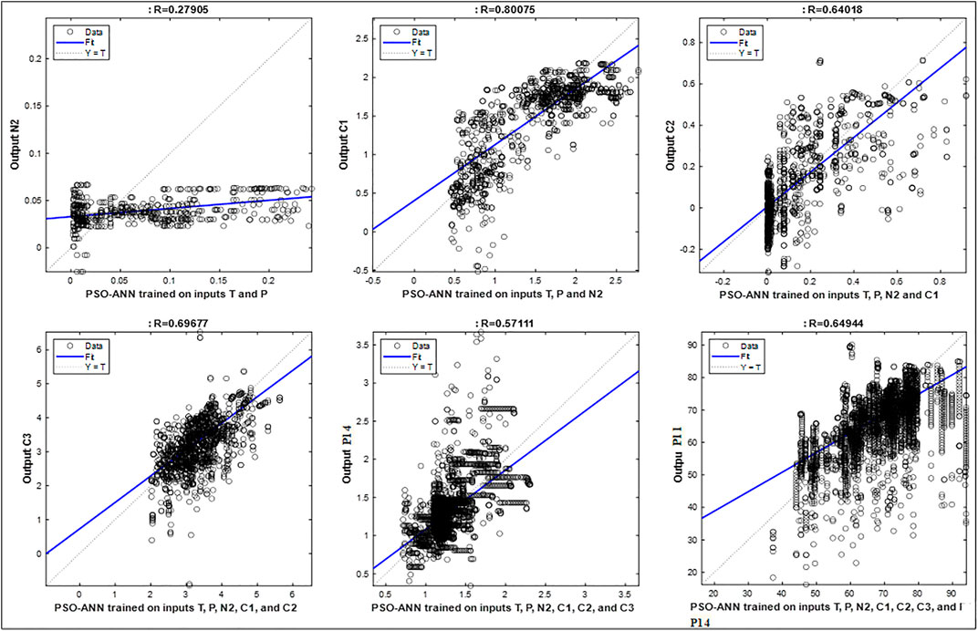
FIGURE 10. Regression relationship between the trained PSO-ANN model and the corresponding dependent variables.
7 Conclusion
NG sources are generally located in remote areas, from which NG is extracted and transported to far-away markets in the form of LNG. The composition and conditions of the extracted NG vary from source to source. These varying conditions can adversely affect the LNG production process, leading to infeasibility. To avoid this problem, a PSO-ANN model is proposed in this study to predict the process behavior in terms of the minimum internal temperature approach (MITA) value at varying decision variables, i.e., NG composition and conditions. The PSO-ANN model showed an 80% success rate for predicting the feasibility of the process through the correct estimation of the decision variables. It was also found that the proposed model is suitable for predicting the feasible set of decision variables, even for unusual sets of user-defined test data. Furthermore, the 20% failure rate may be converted to a success rate by training the model again on a different set of model parameters.
Data Availability Statement
The original contributions presented in the study are included in the article/Supplementary Material; further inquiries can be directed to the corresponding authors.
Author Contributions
All authors listed have made a substantial, direct, and intellectual contribution to the work and approved it for publication.
Funding
This work was supported by the 2021 Yeungnam University Research Grant and by the Priority Research Centre Program through the National Research Foundation of Korea (NRF) funded by the Ministry of Education (2014R1A6A1031189). This work was also supported by the Deanship of Scientific Research at King Khalid University, Abha-KSA, through the General Research Project under grant number (R.G.P. 2/189/43).
Conflict of Interest
The authors declare that the research was conducted in the absence of any commercial or financial relationships that could be construed as a potential conflict of interest.
Publisher’s Note
All claims expressed in this article are solely those of the authors and do not necessarily represent those of their affiliated organizations, or those of the publisher, the editors, and the reviewers. Any product that may be evaluated in this article, or claim that may be made by its manufacturer, is not guaranteed or endorsed by the publisher.
References
Academic, T. M.-P. (1993). Neural Network Recipes in C., and 1993, Undefined Practical Neural Network Recipes in C++. San Diego, CA: Academic Press.
Alam, M., Das, B., and Pant, V. Electric Power Systems Research (2015). Undefined A Comparative Study of Metaheuristic Optimization Approaches for Directional Overcurrent Relays Coordination. Elsevier.
Ali, W., Khan, M. S., Qyyum, M. A., and Lee, M. (2018). Surrogate-Assisted Modeling and Optimization of a Natural-Gas Liquefaction Plant. Comput. Chem. Eng. 118, 132–142. doi:10.1016/j.compchemeng.2018.08.003
Ali, W., Qyyum, M. A., Khan, M. S., Duong, P. L. T., and Lee, M. (2019). Knowledge-Inspired Operational Reliability for Optimal LNG Production at the Offshore Site. Appl. Therm. Eng. 150, 19–29. doi:10.1016/j.applthermaleng.2018.12.165
Amiri, M., Bakhshandeh Amnieh, H., Hasanipanah, M., and Mohammad Khanli, L. (2016). A New Combination of Artificial Neural Network and K-Nearest Neighbors Models to Predict Blast-Induced Ground Vibration and Air-Overpressure. Eng. Comput. 32, 631–644. doi:10.1007/s00366-016-0442-5
Armaghani, D. J., Hajihassani, M., Mohamad, E. T., Marto, A., and Noorani, S. A. (2014). Blasting-Induced Flyrock and Ground Vibration Prediction through an Expert Artificial Neural Network Based on Particle Swarm Optimization. Arab. J. Geosci. 7, 5383–5396. doi:10.1007/s12517-013-1174-0
Aspelund, A., Gundersen, T., Myklebust, J., Nowak, M. P., and Tomasgard, A. (2010). An Optimization-Simulation Model for a Simple LNG Process. Comput. Chem. Eng. 34, 1606–1617. doi:10.1016/j.compchemeng.2009.10.018
Basheer, I. A. (2000). Selection of Methodology for Modeling Hysteresis Behavior of Soils Using Neural Networks. Comput. Aided Civ. Infrastructure 15, 445–463. undefined. doi:10.1111/0885-9507.00206
Cao, L., Liu, J., and Xu, X. (2016). Robustness Analysis of the Mixed Refrigerant Composition Employed in the Single Mixed Refrigerant (SMR) Liquefied Natural Gas (LNG) Process. Appl. Therm. Eng. 93, 1155–1163. doi:10.1016/j.applthermaleng.2015.10.072
Ceryan, N., Okkan, U., and Kesimal, A. (2013). Prediction of Unconfined Compressive Strength of Carbonate Rocks Using Artificial Neural Networks. Environ. Earth Sci. 68, 807–819. doi:10.1007/s12665-012-1783-z
Ghasemi, E. (2017). Particle Swarm Optimization Approach for Forecasting Backbreak Induced by Bench Blasting. Neural Comput. Applic. 28, 1855–1862. doi:10.1007/s00521-016-2182-2
Güllü, H., and Geology, E. E.-E. (2007). A Neural Network Approach for Attenuation Relationships: An Application Using Strong Ground Motion Data from Turkey. Eng. Geol. 93, 65–81. undefined. doi:10.1016/j.enggeo.2007.05.004
Hajihassani, M., Armaghani, D., Sohaei, H., and Acoustics, E. M.-A. (2014). Prediction of Airblast-Overpressure Induced by Blasting Using a Hybrid Artificial Neural Network and Particle Swarm Optimization. Appl. Acoust. 80, 57–67. doi:10.1016/j.apacoust.2014.01.005
Hasan, M. M. F., Karimi, I. A., Alfadala, H. E., and Grootjans, H. (2009). Operational Modeling of Multistream Heat Exchangers with Phase Changes. AIChE J. 55, 150–171. doi:10.1002/aic.11682
He, T., Karimi, I. A., and Ju, Y. (2018). Review on the Design and Optimization of Natural Gas Liquefaction Processes for Onshore and Offshore Applications. Chem. Eng. Res. Des. 132, 89–114. doi:10.1016/j.cherd.2018.01.002
He, T., Liu, Z., Ju, Y., and Parvez, A. M. (2019). A Comprehensive Optimization and Comparison of Modified Single Mixed Refrigerant and Parallel Nitrogen Expansion Liquefaction Process for Small-Scale Mobile LNG Plant. Energy 167, 1–12. doi:10.1016/j.energy.2018.10.169
Hecht-Nielsen, R. (2018). Scanned by CamScanner Kolmogorov's Mapping Neural Network Existence Theorem.
Hornik, K., Stinchcombe, M., and White, H. (1989). Multilayer Feedforward Networks Are Universal Approximators. Neural Netw. 2, 359–366. doi:10.1016/0893-6080(89)90020-8
Hush, D. (1989). “Classification with Neural Networks: A Performance Analysis,” in Proceeding of the IEEE International Conference on Systems Engineering, Fairborn, OH, USA, August 1989 (IEEE).
Jahed Armaghani, D., Hasanipanah, M., Tonnizam Mohamad, E., and Tonnizam Mohamad, E. (2016). A Combination of the ICA-ANN Model to Predict Air-Overpressure Resulting from Blasting. Eng. Comput. 32, 155–171. doi:10.1007/s00366-015-0408-z
Kaastra, I., and Boyd, M. (1996). Designing a Neural Network for Forecasting Financial and Economic Time Series. Neurocomputing 10, 215–236. doi:10.1016/0925-2312(95)00039-9
Kanellopoulos, I., and Wilkinson, G. G. (1997). Strategies and Best Practice for Neural Network Image Classification. Int. J. Remote Sens. 18, 711–725. doi:10.1080/014311697218719
Karlik, B., and Olgac, A. (2010). Performance Analysis of Various Activation Functions in Generalized MLP Architectures of Neural Networks. Int. J. Artif. Intell. Expert Syst. 1, 111–115.
Kesler, M. G., and Lee, B. I. (1975). A Generalized Thermodynamic Correlation Based onThree-Parameter Corresponding States. AIChE J. 21, 510–527. doi:10.1002/aic.690210313
Khan, M. S., Karimi, I. A., and Wood, D. A. (2017). Retrospective and Future Perspective of Natural Gas Liquefaction and Optimization Technologies Contributing to Efficient LNG Supply: A Review. J. Nat. Gas Sci. Eng. 45, 165–188. doi:10.1016/j.jngse.2017.04.035
Lee, G. C., Smith, R., and Zhu, X. X. (2002). Optimal Synthesis of Mixed-Refrigerant Systems for Low-Temperature Processes. Ind. Eng. Chem. Res. 41, 5016–5028. doi:10.1021/ie020057p
Lee, I., Park, J., and Moon, I. (2018). Key Issues and Challenges on the Liquefied Natural Gas Value Chain: A Review from the Process Systems Engineering Point of View. Ind. Eng. Chem. Res. 57, 5805–5818. doi:10.1021/acs.iecr.7b03899
Luu Trung Duong, P., Quang Minh, L., Abdul Qyyum, M., and Lee, M. (2018). Sparse Bayesian Learning for Data Driven Polynomial Chaos Expansion with Application to Chemical Processes. Chem. Eng. Res. Des. 137, 553–565. doi:10.1016/j.cherd.2018.08.006
Meulenkamp, F., and Grima, M. A. (1999). Application of Neural Networks for the Prediction of the Unconfined Compressive Strength (UCS) from Equotip Hardness. Int. J. Rock Mech. Min. Sci. 36, 29–39. doi:10.1016/s0148-9062(98)00173-9
Mohamad, E. T., Jahed Armaghani, D., Momeni, E., and Alavi Nezhad Khalil Abad, S. V. (2015). Prediction of the Unconfined Compressive Strength of Soft Rocks: A PSO-Based ANN Approach. Bull. Eng. Geol. Environ. 74, 745–757. doi:10.1007/s10064-014-0638-0
Mohammad, N., Mohamad Ishak, W. W., Mustapa, S. I., and Ayodele, B. V. (2021). Natural Gas as a Key Alternative Energy Source in Sustainable Renewable Energy Transition: A Mini Review. Front. Energy Res. 9, 237. doi:10.3389/FENRG.2021.625023/BIBTEX
Mokarizadeh Haghighi Shirazi, M., and Mowla, D. (2010). Energy Optimization for Liquefaction Process of Natural Gas in Peak Shaving Plant. Energy 35, 2878–2885. doi:10.1016/j.energy.2010.03.018
Momeni, E., Armaghani, D., Hajihassani, M., and Mohd Amin, M. F. (2015). Prediction of Uniaxial Compressive Strength of Rock Samples Using Hybrid Particle Swarm Optimization-Based Artificial Neural Networks. Measurement 60, 50–63. doi:10.1016/j.measurement.2014.09.075
Mortazavi, A., Alabdulkarem, A., Hwang, Y., and Radermacher, R. (2016). Development of a Robust Refrigerant Mixture for Liquefaction of Highly Uncertain Natural Gas Compositions. Energy 113, 1042–1050. doi:10.1016/j.energy.2016.07.147
Ornek, M., Laman, M., Demir, A., and Yildiz, A. and, and 2012, Prediction of Bearing Capacity of Circular Footings on Soft Clay Stabilized with Granular Soil. Soils Found. 52:69–80.doi:10.1016/j.sandf.2012.01.002
Panigrahi, B., Shi, Y., and Lim, M. (2011). Handbook of Swarm Intelligence: Concepts, Principles and Applications.
Park, J. H., Khan, M. S., and Lee, M. (2015). Modified Coordinate Descent Methodology for Solving Process Design Optimization Problems: Application to Natural Gas Plant. J. Nat. Gas Sci. Eng. 27, 32–41. doi:10.1016/j.jngse.2014.10.014
Park, K., Won, W., and Shin, D. (2016). Effects of Varying the Ambient Temperature on the Performance of a Single Mixed Refrigerant Liquefaction Process. J. Nat. Gas Sci. Eng. 34, 958–968. doi:10.1016/j.jngse.2016.07.069
Peng, D., and Robinson, D. B. (1976). A New Two-Constant Equation of State. Ind. Eng. Chem. Fundam. 15, 59–64. doi:10.1021/i160057a011
Primabudi, E., Morosuk, T., and Tsatsaronis, G. (2019). Multi-Objective Optimization of Propane Pre-Cooled Mixed Refrigerant (C3MR) LNG Process. Energy 185, 492–504. doi:10.1016/j.energy.2019.07.035
Qadeer, K., Qyyum, M. A., and Lee, M. (2018). Krill-Herd-Based Investigation for Energy Saving Opportunities in Offshore Liquefied Natural Gas Processes. Ind. Eng. Chem. Res. 57, 14162–14172. doi:10.1021/acs.iecr.8b02616
Qyyum, M. A., Ali, W., Long, N. V. D., Khan, M. S., and Lee, M. (2018a). Energy Efficiency Enhancement of a Single Mixed Refrigerant LNG Process Using a Novel Hydraulic Turbine. Energy 144, 968–976. doi:10.1016/j.energy.2017.12.084
Qyyum, M. A., Long, N. V. D., Minh, L. Q., and Lee, M. (2018b). Design Optimization of Single Mixed Refrigerant LNG Process Using a Hybrid Modified Coordinate Descent Algorithm. Cryogenics 89, 131–140. doi:10.1016/j.cryogenics.2017.12.005
Qyyum, M. A., Qadeer, K., and Lee, M. (2018c). Comprehensive Review of the Design Optimization of Natural Gas Liquefaction Processes: Current Status and Perspectives. Ind. Eng. Chem. Res. 57, 5819–5844. doi:10.1021/acs.iecr.7b03630
Qyyum, M. A., Duong, P. L. T., Minh, L. Q., Lee, S., and Lee, M. (2019). Dual Mixed Refrigerant LNG Process: Uncertainty Quantification and Dimensional Reduction Sensitivity Analysis. Appl. Energy 250, 1446–1456. doi:10.1016/j.apenergy.2019.05.004
Raja, V., and Rajagopalan, S. (2014). A Comparative Analysis of Optimization Techniques for Artificial Neural Network in Bio Medical Applications. J. Comput. Sci. 10, 106–114. doi:10.3844/jcssp.2014.106.114
Ripley, B. (1993). In aStatistical Aspects of Neural Networks, O Networks on Chaos: Statistical and Probabilistic Aspects. Editors U. Bornndorff-Nielsen, J. Jensen, and W. Kendal.
Rukhaiyar, S., Alam, M. N., and Samadhiya, N. K. (2018). A PSO-ANN Hybrid Model for Predicting Factor of Safety of Slope. Int. J. Geotechnical Eng. 12, 1–11. doi:10.1080/19386362.2017.1305652
Shahin, M. A., Maier, H. R., and Jaksa, M. B. (2002). Predicting Settlement of Shallow Foundations Using Neural Networks. J. Geotech. Geoenvironmental Eng. 128, 785. doi:10.1061/(asce)1090-0241(2002)128:9(785)
Shell LNG outlook (2019). Shell LNG Outlook. Available at: https://www.shell.com/energy-and-innovation/natural-gas/liquefied-natural-gas-lng/lng-outlook-2019.html.
Sonmez, H., Gokceoglu, C., Nefeslioglu, H. A., and Kayabasi, A. (2006). Estimation of Rock Modulus: For Intact Rocks with an Artificial Neural Network and for Rock Masses with a New Empirical Equation. Int. J. Rock Mech. Min. Sci. 43, 224–235. doi:10.1016/j.ijrmms.2005.06.007
Talal, R. (2014). Comparative Study Between the (BA) Algorithm and (PSO) Algorithm to Train (RBF) Network at Data Classification.
Wu, X., Wang, Z., Dai, X., Ge, Q., and Liu, F. (2021). Optimization Design and Analysis of Single-Stage Mixed Refrigerant Liquefaction Process. Front. Energy Res. 9, 626. doi:10.3389/FENRG.2021.766588/BIBTEX
Xie, L., Zhuang, D., Li, Z., and Ding, G. (2022). Technical Characteristics and Development Trend of Printed Circuit Heat Exchanger Applied in Floating Liquefied Natural Gas. Front. Energy Res. 10, 383. doi:10.3389/FENRG.2022.885607
Xiong, X., Lin, W., and Gu, A. (2016). Design and Optimization of Offshore Natural Gas Liquefaction Processes Adopting PLNG (Pressurized Liquefied Natural Gas) Technology. J. Nat. Gas Sci. Eng. 30, 379–387. doi:10.1016/j.jngse.2016.02.046
Yagiz, S., and Gokceoglu, C. (2010). Application of Fuzzy Inference System and Nonlinear Regression Models for Predicting Rock Brittleness. Expert Syst. Appl. 37, 2265–2272. doi:10.1016/j.eswa.2009.07.046
Zhang, J., Meerman, H., Benders, R., and Faaij, A. (2020). Comprehensive Review of Current Natural Gas Liquefaction Processes on Technical and Economic Performance. Appl. Therm. Eng. 166, 114736. doi:10.1016/j.applthermaleng.2019.114736
Nomenclature
NG natural gas
LNG liquefied natural gas
PSO particle swarm optimization
ANN artificial neural network
SMR single mixed refrigerant
TAC total annualized costs
GA genetic algorithm
MITA minimum internal temperature approach
BP back-propagation
MCD modified coordinate descent
PRICO poly-refrigerant integrated cycle operation
LM Levenberg–Marquardt
RMSE root mean square error
Keywords: artificial neural network, natural Gas, single mixed refrigerant, particle swarm optimization, aspen HYSYS
Citation: Ahmad A, Qadeer K, Naquash A, Riaz F, Hasan M, Qyyum MA and Lee M (2022) Particle Swarm-Assisted Artificial Neural Networks for Making Liquefied Natural Gas Processes Feasible Under Varying Feed Conditions. Front. Energy Res. 10:917656. doi: 10.3389/fenrg.2022.917656
Received: 11 April 2022; Accepted: 25 May 2022;
Published: 11 July 2022.
Edited by:
Muhammad Wakil Shahzad, Northumbria University, United KingdomReviewed by:
Arnab Dutta, Birla Institute of Technology and Science, IndiaHamid Reza Rahbari, Ferdowsi University of Mashhad, Iran
Copyright © 2022 Ahmad, Qadeer, Naquash, Riaz, Hasan, Qyyum and Lee. This is an open-access article distributed under the terms of the Creative Commons Attribution License (CC BY). The use, distribution or reproduction in other forums is permitted, provided the original author(s) and the copyright owner(s) are credited and that the original publication in this journal is cited, in accordance with accepted academic practice. No use, distribution or reproduction is permitted which does not comply with these terms.
*Correspondence: Muhammad Abdul Qyyum, bS5xeXl1bUBzcXUuZWR1Lm9t; Moonyong Lee, bXlubGVlQHl1LmFjLmty
†These authors have contributed equally to this work