Solving stochastic hydro unit commitment using benders decomposition and modified stochastic dual dynamic programming

This paper proposes a stochastic hydro unit commitment (SHUC) model for a price-taker hydropower producer in a liberalized market. The objective is to maximize the total revenue of the hydropower producer, including the immediate revenue, future revenue (i.e., opportunity cost), and startup and shutdown cost. The market price uncertainty is taken into account through the scenario tree. The solution of the model is a challenging task due to its non-convex and high-dimensional characteristics. A solution method based on the Benders Decomposition (BD) and Modified Stochastic Dual Dynamic Programming (MSDDP) is proposed to solve the problem efficiently. Firstly, the BD is applied to decompose the original problem into a Benders master problem representing the hydro unit commitment and a Benders subproblem representing the optimal operation of the hydropower plants. The Benders subproblem, which contains a large number of integer variables, is further decomposed by the period and solved by the MSDDP proposed in this paper. Finally, we verify the effectiveness of the SHUC model and the performance of the proposed solution method in case studies.

1 Introduction

The hydro unit commitment (HUC) problem is a significant operational problem in the hydropower system (Li et al., 2014). It is used to determine an optimal commitment schedule of each unit in the hydropower plant for the next day or week while considering various physical constraints, such as water balance and minimum up and down time (Nazari-Heris et al., 2017; Ackooij et al., 2021; Amani and Alizadeh, 2021). Due to its non-convex and high-dimensional characteristics, the HUC problem has always been a challenging task (Cheng et al., 2016; Ackooij et al., 2018).

Due to the potential benefits of the HUC problem, a variety of research has been proposed on the HUC problem over the last few decades, mainly focused on the modeling and solution methods (Parvez et al., 2019; Kong et al., 2020). Much literature takes water consumption minimization as the optimization objective (Li et al., 2014; Cheng et al., 2016; Nazari-Heris et al., 2017; Ackooij et al., 2018; Ackooij et al., 2021; Amani and Alizadeh, 2021), and most of the existing models are deterministic (Li et al., 2014; Cheng et al., 2016; Nazari-Heris et al., 2017; Ackooij et al., 2018; Parvez et al., 2019; Kong et al., 2020; Thaeer Hammid et al., 2020; Ackooij et al., 2021; Amani and Alizadeh, 2021). In a liberalized market, a hydropower producer is usually an entity owning hydropower units and participating in the electricity market with the objective of maximizing its total revenue. The hydropower producer obtains the power generation right and gains profit by submitting bidding to the independent system operator (ISO). The ISO is responsible for market clearing and calculating the electricity price at each time. Therefore, the uncertainty of the market price has a significant impact on the HUC schedule (Wei et al., 2021; Xiao et al., 2021). On the other hand, due to the existence of the reservoir, the hydropower producer can release water at the current stage (which gains immediate revenue) or at a certain stage in the future (which gains future revenue). That is, the immediate revenue represents the revenue that the hydropower producer obtains in the current stage by power generation (Kelman et al., 1998). The future revenue represents the economic value of the water stored in the reservoir. To maximize the total revenue, the HUC schedule needs to make a trade-off between the immediate revenue and future revenue (i.e., opportunity cost). A coordinated scheduling method of the wind-hydro system was proposed in (Abreu et al., 2012). The scheduling method was formulated as a stochastic price-based unit commitment model, which maximizes the immediate revenue of the generation company. Literature (Pérez-Díaz et al., 2010) proposed a dynamic programming model to solve the short-term scheduling problem of a hydropower plant that participates in a liberalized market with the objective of maximizing the immediate revenue. The calculation method of the future revenue was firstly proposed in (Kelman et al., 1998). In the paper, the Stochastic dynamic programming (SDP) was applied to calculate the future revenue of a hydrothermal system in the liberalized market. However, the curse of dimensionality of the SDP limited the further application. Then Stochastic dual dynamic programming (SDDP) proposed in (Pereira and Pinto, 1991) was applied in (Kelman et al., 1998; Pereira et al., 1999; Barroso et al., 2002; Helseth et al., 2016) to calculate the future revenue in a large hydropower system. To the best of our knowledge, none of the existing literature on HUC has taken the future revenue into account.

Due to the nature of non-convexity, the solution of the HUC problem has always been a difficulty. Researchers have developed various solution methods to solve it efficiently (Parvez et al., 2019; Kong et al., 2020; Thaeer Hammid et al., 2020). Conventional methods based on mathematical programming primarily include mixed-integer linear programming (MILP) (Diniz and Maceira, 2008; Tong et al., 2013; Guisández and Pérez-Díaz, 2021), non-linear programming (NLP) (Lima et al., 2013), mixed-integer quadratic programming (MIQP) (Finardi and da Silva, 2006), and dynamic programming (DP) (Seguin et al., 2016). Heuristic algorithms such as artificial neural networks (ANN) (Naresh and Sharma, 2000), genetic algorithm (GA) (Ahmed and Sarma, 2005), and differential evolutionary (DE) (Zha ng et al., 2013) were also reported. We refer to (Parvez et al., 2019; Kong et al., 2020; Thaeer Hammid et al., 2020) for more solution methods on the HUC problem. Recently, decomposition methods, including dual decomposition (Finardi and da Silva, 2006), Benders Decomposition (BD) (Benders, 2005; Moiseeva and Hesam zadeh, 2017; Colonetti and Finardi, 2021), and SDDP (Helseth et al., 2016; Hjelmeland et al., 2019) have gained more and more attention in the hydropower generation scheduling problems due to their good computational performance. SDDP is a state-of-the-art algorithm for long- and medium-term hydropower scheduling problems (Hjelmeland et al., 2019). However, SDDP uses the dual solution to construct the future cost function (FCF), so it cannot be used to solve MILP problems (Hjelmeland et al., 2019). The optimal operation of the hydropower plant is a typical non-convex optimization problem. To tackle this difficulty, the McCormick envelope was used by (Cerisola et al., 2012) to approximate the bilinear relationship between variables. Literature (Steeger and Rebennack, 2017) proposed a Lagrangian relaxation of the non-convex SDDP subproblem, and then Lagrange multipliers instead of dual multipliers were used to construct valid FCF. Recently, literature (Zou et al., 2019) proposed a Stochastic Dual Dynamic integer Programming (SDDiP) algorithm for solving multi-stage stochastic integer programming problems with binary state variables. However, SDDiP has to solve a Lagrangian dual problem at each stage. It is well known that the convergence of the Lagrangian dual problem can be very slow. A novel type of cut called locally valid cut was proposed by (Abgottspon et al., 2014) and introduced to the SDDP framework to enhance a convexified approximation of the FCF. The above references propose different approaches to deal with non-convexity in the SDDP subproblem. The ultimate purpose of these approaches is to construct a valid and tight FCF.

The contributions of this paper are listed as follows.

1) A stochastic hydro unit commitment (SHUC) model is proposed, which aims to maximize the hydropower producer’s total revenue. The opportunity cost and the market price uncertainty are taken into account.

2) A solution method, which decomposes the SHUC problem into two layers, is proposed based on the framework of Benders Decomposition. The outer layer is the Benders master problem, which is used to determine each unit’s startup and shutdown status. The inner layer Benders subproblem is used to determine the optimal operation of the hydropower plants.

3) To efficiently solve the large-scale mixed-integer Benders subproblem, a modified stochastic dual dynamic programming (MSDDP) is proposed based on the Lift-and-Project cutting plane (LAPCP) algorithm.

The rest of the paper is organized as follows. Section 2 proposes the SHUC model. Section 3 proposes the solution method of the SHUC model. In Section 4, we verify the effectiveness of the SHUC model and the computational performance of the solution method in case studies. Finally, Section 5 concludes this paper.

2 Stochastic unit commitment model

2.1 Objective function

In a liberalized market, the objective of the SHUC model is to maximize the total revenue, which can be shown in (Eqs 1–4):

$\max F=\left(R^{\mathbf{im}}+R^{\mathbf{fut}}-C\right)(1)$

$R^{\mathbf{im}}={\displaystyle \sum _{t=1}^T{\displaystyle \sum _{k=1}^K{\displaystyle \sum _{j=1}^{J_k}{\theta }_t{P}_{t,k,j}}}}(2)$

$R^{\mathbf{fut}}={\displaystyle \sum _{k=1}^K{\alpha }_k\left(v_{T,k}\right)}(3)$

$C={\displaystyle \sum _{t=1}^T{\displaystyle \sum _{k=1}^K{\displaystyle \sum _{j=1}^{J_k}\left[S{U}_{k,j}z{u}_{t,k,j}+S{D}_{k,j}z{d}_{t,k,j}\right]}}}(4)$

Where $R^{\mathbf{im}}$, $R^{\mathbf{fut}}$, and C represent the immediate revenue, future revenue, and the sum of the startup and shutdown cost, respectively. T, K, and $J_k$ represent the number of periods, hydropower plants, and units in plant k, respectively. We use ${\theta }_t$ to denote the random variable of market price at period t. $P_{t,k,j}$ represents the power output of unit j in plant k. ${\alpha }_k$ represents the piecewise linear approximation of the future revenue (Moiseeva and Hesam zadeh, 2017), which represents the opportunity cost of the water stored in the reservoirs. It is expressed as a function of the reservoir volumes. $S{U}_{k,j}$ and $S{D}_{k,j}$ represent the startup and shutdown cost of unit j in plant k, respectively. $z{u}_{t,k,j}$ is a binary variable that is equal to 1 if unit j is started up and $z{d}_{t,k,j}$ is a binary variable that is equal to 1 if unit j is shut down.

2.2 Constraints

1) Water balance constraint

$v_{t,k}=v_{t-1,k}+3600\mathrm{\Delta }t\left(-q_{t,k}+I_{t,k}+{\displaystyle \sum _{{\omega }_k\in {\Omega }_k}{q}_{t-\tau ,{\omega }_k}}\right),\forall t,\forall k(5)$

Constraint (Eq. 5) represents the water balance equation between two consecutive periods. Where $v_{t,k}$, $q_{t,k}$ and $I_{t,k}$ represent the reservoir volume, water release, and inflow, respectively. $\mathrm{\Delta }t$ represents the number of hours in one period. ${\Omega }_k$ is the set of hydropower plants which are located upstream of the plant k. $\tau$ represents the water delay time between two adjacent plants.

2) Water release, water discharge and spillage

$q_{t,k}=u_{t,k}+s{p}_{t,k},\forall t,\forall k(6)$

$u_{t,k}={\displaystyle \sum _{j=1}^{J_k}{r}_{t,k,j}},\forall t,\forall k(7)$

$0\le r_{t,k,j}\le z_{t,k,j}{R}_{k,j}^{\max },\forall t,\forall k,\forall j(8)$

Constraint (Eq. 6) defines the relationship between water release, water discharge, and spillage. Constraint (Eq. 7) gives the expression of the water discharge. Constraint (Eq. 8) defines the upper and lower bounds on unit discharge. Where $u_{t,k}$ and $s{p}_{t,k}$ represent the water discharge and spillage, respectively. $r_{t,k,j}$ represents the water discharge of unit j in plant k. $z_{t,k,j}$ is a binary variable that is equal to 1 if unit j is online. $U_{k,j}^{\max }$ represents the maximum of the water discharge of unit j.

3) Fore-bay level, tail-race level, penstock loss, and net head

$h{u}_{t,k}=f{u}_k\left({\overline{v}}_{t,k}\right),\forall t,\forall k(9)$

${\overline{v}}_{t,k}=\frac{v_{t-1,k}+v_{t,k}}{2},\forall t\left\{2,\dots ,24\right\},\forall k(10)$

$h{d}_{t,k}=f{d}_k\left(q_{t,k}\right),\forall t,\forall k(11)$

$h{l}_{t,k,j}=f{l}_{k,j}\left(r_{t,k,j}\right),\forall t,\forall k,\forall j(12)$

$h_{t,k,j}=h{u}_{t,k}-h{d}_{t,k}-h{l}_{t,k,j},\forall t,\forall k,\forall j(13)$

The fore-bay level is formulated as a non-linear function of the reservoir volume (Li et al., 2014), as shown in (Eq. 9). Constraint (Eq. 10) defines the medium volume as the average reservoir volume in two consecutive periods (Pereira et al., 2017). The tail-race level is formulated as a nonlinear function of the water release (Li et al., 2014), as given in (Eq. 11). Constraint (Eq. 12) gives the relationship between the penstock loss and unit discharge (Cheng et al., 2016). Constraint (Eq. 13) defines the expression of the net head. Where $h{u}_{t,k}$ and $h{d}_{t,k}$ represent the fore-bay and tail-race levels of plant k, respectively. $h{l}_{t,k,j}$ and $h_{t,k,j}$ represent the penstock loss and net head of the unit j in plant k, respectively.

4) Future revenue constraints

${\alpha }_k\le {\displaystyle \sum _{k=1}^K{\pi }_{w,k}{v}_{T,k}}+{\beta }_w,w\in \mathrm{\Phi },\forall k(14)$

Constraint (Eq. 14) defines the future revenue of the hydropower producer. Where ${\pi }_{w,k}$ and ${\beta }_w$ denote the slope and intercept of the future revenue, respectively. $v_{T,k}$ represents the reservoir volume at period T. $\Phi$ represents the set of the slope index. The future revenue is expressed as a piecewise linear function of the reservoir volume. It can be obtained by the medium-term scheduling using SDDP. We refer to (Kelman et al., 1998) for more details.

5) Hydropower generation function

$P_{t,k,j}=f{p}_{k.j}\left(r_{t,k,j},h_{t,k,j},{\eta }_{k,j}\right),\forall t,\forall k,\forall j(15)$

${\eta }_{k,j}=f{e}_{k,j}\left(r_{t,k,j},h_{t,k,j}\right),\forall t,\forall k,\forall j(16)$

$0\le P_{t,k,j}\le z_{t,k,j}{P}_{k,j}^{\max },\forall t,\forall k,\forall j(17)$

The hydropower generation function is a non-linear function of the unit discharge, generation efficiency, and net head (Cheng et al., 2016), as shown in (Eq. 15). The generation efficiency of the hydro unit is a non-linear function of the unit discharge and net head (Cheng et al., 2016), as defined in (Eq. 16). Where ${\eta }_{k,j}$ represents the generation efficiency of the unit j. The non-linear relationships in (Eqs 9, 11, 12, 15, 16) can be linearized using the method proposed in (Guisández and Pérez-Díaz, 2021).

7) Forbidden operation zones

$P_{t,k,j}-{\underset{¯}{F}}_{k,j}-{\overline{P}}_{k,j}\left(1-z{o}_{t,k,j}\right)\le 0,\forall t,\forall k,\forall j(18)$

$P_{t,k,j}-{\overline{F}}_{k,j}\left(1-z{o}_{t,k,j}\right)\ge 0,\forall t,\forall k,\forall j(19)$

Constraints (Eq. 18) and (Eq. 19) define the constraints of the forbidden operation zones on the hydro unit. Where $\left[{\underset{¯}{F}}_{k,j},{\overline{F}}_{k,j}\right]$ is the forbidden power output of unit j. $z{o}_{t,k,j}$ is a binary variable that is equal to 1 if $0\le P_{t,k,j}\le {\underset{¯}{F}}_{k,j}$ and 0 if ${\overline{F}}_{k,j}\le P_{t,k,j}\le {\overline{P}}_{k,j}$.

6) Logical constraints

$z_{t,k,j}-z_{t-1,k,j}=z{u}_{t,k,j}-z{d}_{t,k,j},\forall t,\forall k,\forall j(20)$

$z{u}_{t,k,j}+z{d}_{t,k,j}\le 1,\forall t,\forall k,\forall j(21)$

$z{u}_{t,k,j}+{\displaystyle \sum _{\tau =t+1}^{t+UT-1}z{d}_{t,k,j}}\le 1,\forall t,\forall k,\forall j(22)$

$z{d}_{t,k,j}+{\displaystyle \sum _{\tau =t+1}^{t+DT-1}z{u}_{t,k,j}}\le 1,\forall t,\forall k,\forall j(23)$

${\displaystyle \sum _{t=1}^{T}z{u}_{t,k,j}\le ZU},\forall t,\forall k,\forall j(24)$

${\displaystyle \sum _{t=1}^{T}z{d}_{t,k,j}\le ZD},\forall t,\forall k,\forall j(25)$

Constraints (Eq. 20) and (Eq. 21) define the startup and shutdown statuses of the unit j. Constraints (Eq. 22) and (Eq. 23) guarantee the minimum online/offline time of the unit j. Constraints (Eq. 24) and (Eq. 25) limit the maximum numbers of startup and shutdown, respectively. Where UT and DT represent the minimum online and offline time of the unit, respectively. ZU and ZD represent the number of the startup and shutdown of the unit, respectively.

3 Solution method

The SHUC model proposed in Section 2 contains a large number of integer variables. The solution time increases exponentially when the number of scenarios increases. SDDP is an efficient decomposition algorithm for solving multi-stage stochastic programming problems. However, the multiperiod coupling constraints (Eqs 22–25) and integer variables make the SDDP algorithm unable to be applied directly.

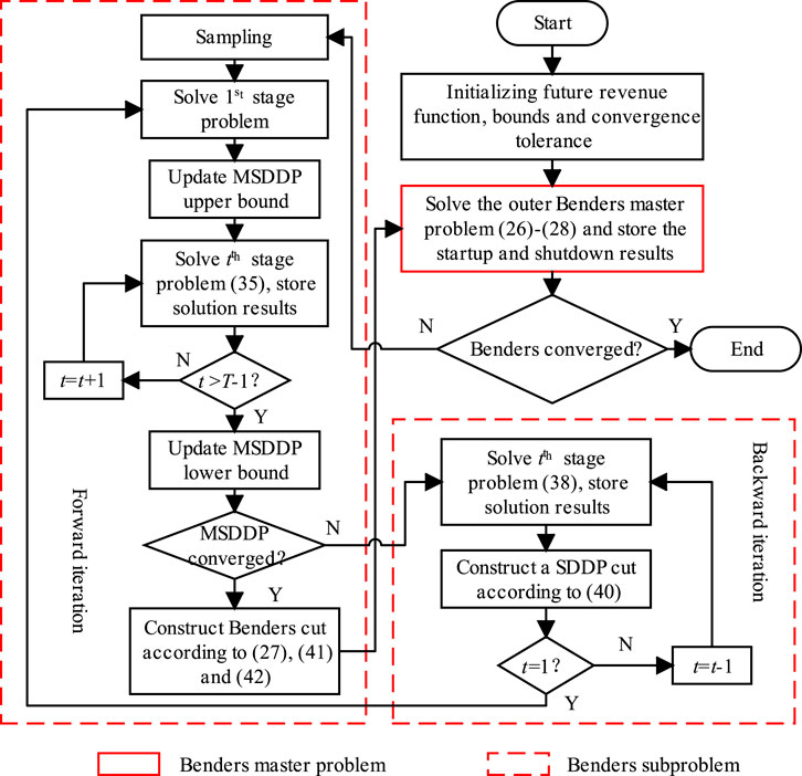
This section proposes a two-layer decomposition solution method based on the BD and MSDDP. We first use the BD to deal with multiperiod coupling constraints. The original problem (Eqs 1–25) is decomposed into a Benders master problem (BMP) [as shown in (Eqs 26–28)] and a Benders subproblem (BSP) [as shown in (Eqs 29–34)]. Then, the BSP is further decomposed according to the period and solved by the MSDDP algorithm proposed in Section 3.2. In each iteration, the BMP provides the startup and shutdown statuses for the BSP, while the BSP decides the optimal operation schedule of each unit and feeds back the parameters used to construct the Benders cut.

The solution method proposed in this section is conceptually similar to the work proposed in (Helseth et al., 2018), the differences between the two methods are listed as follows. 1) The binary variables related to the water level constraints are included in the BSP to provide information for the optimization of the BSP. Therefore, the BSP is formulated as a MILP problem, which cannot be solved by the SDDP. That is, the solution method proposed in (Helseth et al., 2018) will no longer work here. 2) The proposed method solves the BSP to optimal in each iteration of the BD algorithm. Therefore, the cut generated by the BSP is tighter than the method in (Helseth et al., 2018), which leads to a shorter solution time.

To avoid confusion, the cut provided for the BMP is called Benders cut, as shown in (Eq. 27). The cut generated in the backward iteration of the MSDDP is called MSDDP cut, as shown in.

3.1 The outer layer BD algorithm

The BMP is shown in (Eqs 26–28):

$\max \left[\chi -{\displaystyle \sum _{t=1}^T{\displaystyle \sum _{k=1}^K{\displaystyle \sum _{j=1}^{J_k}\left(S{U}_{k,j}z{u}_{t,k,j}+S{D}_{k,j}z{d}_{t,k,j}\right)}}}\right](26)$

$\chi -{\displaystyle \sum _{t=1}^T{\displaystyle \sum _{k=1}^K{\displaystyle \sum _{j=1}^{J_k}{\sigma }_{t,k,j}{z}_{t,k,j}}}}\le l(27)$

$\left(20\right)-\left(25\right)(28)$

Where $\chi$ is a continuous variable representing the objective value of the inner layer BSP. ${\sigma }_{t,k,j}$ and l represent the slope and intercept of the Benders cut, respectively. The calculation of ${\sigma }_{t,k,j}$ and l are discussed in Section 3.2.

The BSP is shown in (Eqs 29–34):

$\max R={\displaystyle \sum _{t=1}^T{\displaystyle \sum _{k=1}^K{\displaystyle \sum _{j=1}^{J_k}{\theta }_t{P}_{t,k,j}}}}+{\displaystyle \sum _{k=1}^K{\alpha }_k\left(v_{T,k}\right)}(29)$

$\left(5\right)-\left(19\right)(30)$

$m_{t,k,j}={\tilde{z}}_{t,k,j}\text{:}\left({\tau }_{t,k,j}\right),\forall t,\forall k,\forall j(31)$

$0\le r_{t,k,j}\le m_{t,k,j}{U}_{k,j}^{\max },\forall t,\forall k,\forall j(32)$

$0\le P_{t,k,j}\le m_{t,k,j}{P}_{k,j}^{\max },\forall t,\forall k,\forall j(33)$

$m_{t,k,j}\in \left[\mathrm{0,1}\right],\forall t,\forall k,\forall j(34)$

Where ${\tilde{z}}_{t,k,j}$ represents the unit startup/shutdown status determined in the BMP. ${\tau }_{t,k,j}$ represents the dual variable of the corresponding constraint.

3.2 The inner layer MSDDP algorithm

We denote the stochastic process of market price by $\left({\theta }_1,\dots ,{\theta }_T\right)$, with ${\theta }_1$ being deterministic. We assume the stochastic process $\left({\theta }_1,\dots ,{\theta }_T\right)$ is stagewise independent. This allows cut sharing between different MSDDP subproblems (Hjelmeland et al., 2019). The stochastic process can be discretized to a scenario tree, in which the realizations in each period are finite, as shown in Figure 1. The number of scenarios in the complete scenario tree is $N={\displaystyle {\prod }_{t=2}^T{N}_t}$. $N_t$ is the number of realizations at period t. This results in replacing the BSP (Eqs 29–34) with the sample average approximation (SAA) problem (Birge and Louveaux, 2011), which can be solved by the MSDDP algorithm proposed in this section.

FIGURE 1

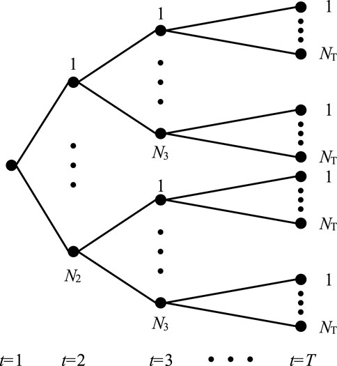
FIGURE 1. The complete scenario tree.

The main idea of the MSDDP contains four parts: convergence criterion, sampling, forward iteration, and backward iteration. The first three parts is similar to the well-known SDDP. For more details, we refer to (Shapiro, 2011).

In the backward iteration of the classical SDDP algorithm, the SDDP cuts are generated using the dual variables of the state transition equation (Pereira and Pinto, 1991; Shapiro, 2011). However, the information of dual variables is unavailable due to the existence of integer variables in (Eq. 30). Inspired by (Balas et al., 1993; Balas et al., 1996), the Lift-and-Project cutting plane algorithm (LAPCP) is developed here to solve the mixed-integer BSP problem through its LP relaxation at each stage. Lift-and-Project cuts are sequentially added to the LP relaxation problem to ensure its optimal solution is the same as the original mixed-integer problem. Finally, the MSDDP cut is generated using the dual solution of the linear relaxation problem.

For ease of presentation, the general mathematical form of the BSP at tth stage can be stated as

$\begin{array}{l}\max c_{t,s}^T{x}_{t,s}+d_{t,s}^T{y}_{t,s}+{\psi }_t\left(x_{t,s}\right)\\ \mathrm{s}\mathrm{.t}\mathbf{.}{B}_{t,s}{x}_{t-1,s}+A_{t,s}{x}_{t,s}+C_{t,s}{y}_{t,s}\ge b_{t,s}\\ x_{t-1,s},x_{t,s}\in {\left\{\mathrm{0,1}\right\}}^n\end{array}(35)$

$\begin{array}{l}{\psi }_t\left(x_{t,s}\right)=\max c_{t+1,s}^T{x}_{t+1,s}+d_{t+1,s}^T{y}_{t+1,s}+{\psi }_{t+1}\left(x_{t+1,s}\right)\\ \mathrm{s}\mathrm{.t}\mathbf{.}{B}_{t+1,s}{x}_{t,s}+A_{t+1,s}{x}_{t+1,s}+C_{t+1,s}{y}_{t+1,s}\ge b_{t+1,s}\\ x_{t,s},x_{t+1,s}\in {\left\{\mathrm{0,1}\right\}}^n\end{array}(36)$

Where s is the scenario index. $x_{t,s}$ and $y_{t,s}$ represent the integer variable and continuous variable, respectively. ${\psi }_t\left(x_{t,s}\right)$ is the future revenue of the tth stage problem. The feasible set of the problem (Eq. 35) is represented as $M_t$. The linear relaxation of $M_t$ is $Y_t$.

The convex hull of the feasible set of (Eq. 35) can be stated as

$D_t=\mathrm{conv}\left\{\begin{array}{l}\left(x_{t-1,s},x_{t,s},y_{t,s}\right):B_{t,s}{x}_{t-1,s}+A_{t,s}{x}_{t,s}+C_{t,s}{y}_{t,s}\ge b_{t,s},\\ x_{t-1,s},x_{t,s}\in {\left\{\mathrm{0,1}\right\}}^n\end{array}\right\}(37)$

According to (Balas, 2011), the optimal solution of (Eq. 38) solves (Eq. 35).

$\begin{array}{l}\max c_{t,s}^T{x}_{t,s}+d_{t,s}^T{y}_{t,s}+{\psi }_t\left(x_{t,s}\right)\\ \mathrm{s}\mathrm{.t}\mathbf{.}\left(x_{t-1,s},x_{t,s},y_{t,s}\right)\in D_t\end{array}(38)$

However, the exact expression of $D_t$ is extremely difficult to obtain due to the exponential dimensions of the problem (Balas, 2011). The LAPCP algorithm is an exact algorithm for solving the MILP problem (Balas et al., 1993). The main idea of LAPCP is to solve the LP relaxation of the original mixed-integer problem (Eq. 35). In each iteration, a Lift-and-Project cut (LPA cut), which cuts off part of $Y_t$, but no point of $M_t$, is generated and added to the LP relaxation problem to approximate $D_t$. The virtue of the LAPCP algorithm allows us to solve (Eq. 35) through the corresponding LP relaxation problem (Eq. 39) in a sequential manner. The flow chart of the LAPCP algorithm for solving the problem (Eq. 39) is shown in Figure 2.

$\begin{array}{l}\max c_{t,s}^T{x}_{t,s}+d_{t,s}^T{y}_{t,s}+{\psi }_t^i\left(x_{t,s}\right)\\ \mathrm{s}\mathrm{.t}\mathbf{.}{A}_{t,s}{x}_{t,s}+C_{t,s}{y}_{t,s}\ge b_{t,s}-B_{t,s}{\widehat{x}}_{t-1,s}\left({\mathit{\vartheta }}_{t,s,1}\right)\\ {\pi }_{t,s}^i{x}_{t,s}+{\lambda }_{t,s}^i{y}_{t,s}\ge {\delta }_{t,s}^i-{\kappa }_{t,s}^i{\widehat{x}}_{t-1,s},i=1,\dots ,I\left({\mathit{\vartheta }}_{t,s,2}^i\right)\\ x_{t,s}\in \left[\mathrm{0,1}\right]\end{array}(39)$

Where ${\widehat{x}}_{t-1,s}$ is the trial value provided by the forward iteration of the MSDDP. ${\pi }_{t,s}^i$, ${\lambda }_{t,s}^i$, ${\kappa }_{t,s}^i$ and ${\delta }_{t,s}^i$ are parameters of the LAP cut. ${\vartheta }_{t,s,1}$ and ${\vartheta }_{t,s,2}$ are dual variables of the corresponding constraints. I represents the number of the LAP cuts.

FIGURE 2

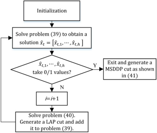
FIGURE 2. The flow chart of the LAPCP algorithm for solving the problem (39).

The parameters of the LAP cut can be obtained by solving (Eq. 40) (Balas et al., 1993).

$\begin{array}{l}\min {\kappa }_{t,s}^i{\widehat{x}}_{t-1,s}^i+{\pi }_{t,s}^i{\widehat{x}}_{t,s}^i+{\lambda }_{t,s}^i{\widehat{y}}_{t,s}^i-{\delta }_{t,s}^i\\ \mathrm{s}\mathrm{.t}\mathbf{.}{\kappa }_{t,s}^i-u_{t,s}^1{B}_{t,s}\ge 0\\ {\sigma }_{t,s}^i-u_{t,s}^{0}e-u_{t,s}^1{W}_{t,s}\ge 0\\ {\kappa }_{t,s}^i-v_{t,s}^1{B}_{t,s}\ge 0\\ {\sigma }_{t,s}^i-v_{t,s}^{0}e-v_{t,s}^1{W}_{t,s}\ge 0\\ -{\delta }_{t,s}^i+v_{t,s}^1{b}_{t,s}+v_{t,s}^0\ge 0\\ u_{t,s}^{1}e+u_{t,s}^0+v_{t,s}^{1}e+v_{t,s}^0=1\\ u_{t,s}^0,u_{t,s}^1,v_{t,s}^0,v_{t,s}^1\ge 0\end{array}(40)$

Where $W_{t,s}=\left[A_{t,s},C_{t,s}\right]$. $u_{t,s}^1$ and $v_{t,s}^1$ are vectors. $u_{t,s}^0$ and $v_{t,s}^0$ are scalars. $e$ is a compatible vector of ones.

The proposed MSDDP algorithm is shown in Table 1. Given ${\widehat{x}}_{t-1,s}$, (Eq. 39) is a LP problem, which indicates that the MSDDP cut can be obtained by solving the corresponding LP dual problem. Therefore, the MSDDP cut of the t-1 stage problem can be generated according to (Eq. 41).

${\phi }_{t-1}\le \frac{1}{N_t}{\displaystyle \sum _{s=1}^{N_t}\left[{\vartheta }_{t,s,1}\left(b_{t,s}-B_{t,s}{x}_{t-1,s}\right)+{\displaystyle \sum _{i=1}^I{\vartheta }_{t,s,2}^i\left({\delta }_{t,s}^i-{\kappa }_{t,s}^i{x}_{t-1,s}\right)}\right]}(41)$

TABLE 1

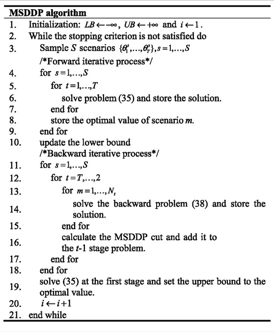
TABLE 1. The flow chart of the MSDDP algorithm.

When the BSM (i.e., the MSDDP algorithm) converges, the Benders cut can be calculated, as shown in (Eq. 27). The calculation of ${\sigma }_{t,k,j}$ and l are shown as follows:

${\sigma }_{t,k,j}=\frac{1}{N_t}{\displaystyle \sum _{s=1}^{N_t}{\tau }_{t,k,j,s},}\forall t,\forall k,\forall j(42)$

$l=R_1-{\displaystyle \sum _{t=1}^T{\displaystyle \sum _{k=1}^K{\displaystyle \sum _{j=1}^{J_k}{\sigma }_{t,k,j}{\tilde{z}}_{t,k,j}^{\mathbf{B}}}}}(43)$

Where $R_1$ represents the optimal value of the inner layer problem at the first stage. To sum up, the flow chart of the proposed solution method to solve the problem (Eqs 1–25) is shown in Figure 3.

FIGURE 3

FIGURE 3. The flow chart of the proposed solution method to solve the problem (1)–(25).

4 Case study

4.1 Basic data

To verify the effectiveness of the proposed SHUC model and solution method. Two realistic case studies are used: the Xiluodu and Xiangjiaba hydropower system (in Sections 4.2.1–4.2.3) and a bigger hydropower system (in Section 4.2.4) reported in (Conejo et al., 2002).

The Xiluodu and Xiangjiaba hydropower system, which includes two hydropower plants (hereinafter referred to as plant Xi and plant Xiang), is located on the Yangtze River, Sichuan Province, in southwestern China. The Xiluodu plant is the third-largest hydropower plant in the world. It is an annual regulation plant that contains 18 large-size units with a total capacity of 12,600 MW. The Xiangjiaba plant, which is located downstream of the Xiluodu plant, includes 8 units with a total capacity of 6,000 MW (Peng et al., 2015). The main technical parameters of the two plants are shown in Table 2. For simplicity, the number of startup and shutdown of the unit is two, and the minimum startup and shutdown time is assumed to be 4 h. The forbidden operation zones of the units are assumed to be $\left[\mathrm{0,0.2}{P}^{\max }\right]$. The start-up and shutdown costs are 300 $/time and 100 $/time, respectively. The convergence tolerance of the outer layer BD algorithm is set as 0.01%. The parameters of the future revenue constraints (Eq. 14) are shown in Table 3. The initial reservoir volumes are 69.0e8 m³ and 45.0e8 m³, respectively. It should be noted that the termination volumes of the two reservoirs are not set. In Section 4.2.2, we show that due to the existence of the future revenue constraints (Eq. 14), the plants terminated discharging at optimal volumes, at which the total revenue of the hydropower producer is maximized.

TABLE 2

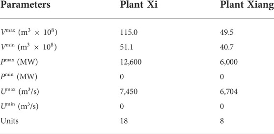
TABLE 2. Technical parameters of the hydropower plants.

TABLE 3

TABLE 3. The parameters of the future revenue constraints.

The generation of the scenario tree includes three steps (Heitsch and Römisch, 2003), as shown in Figure 4. 1) Price forecast. The market price is forecasted using the autoregressive moving average (ARMA) model. 2) Probability distribution estimation. The Pearson 3 distribution is used for probability distribution estimation of the forecast error. The parameter of the probability density function (pdf) of the Pearson 3 distribution is estimated using the historical day-ahead market price of Sichuan Province. 3) Scenario generation. The Monte Carlo sampling method is used to generate discretized scenarios from the forecast price and pdf.

FIGURE 4

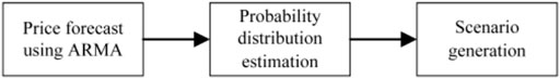
FIGURE 4. The procedure of the scenario tree generation.

A time horizon of 1 day is considered with hourly time steps. Three price nodes are considered at each period, with a total of $3^{23}$ scenarios in the complete scenario tree. The problem scale of the proposed SHUC model in the complete scenario tree is shown in Table 4.

TABLE 4

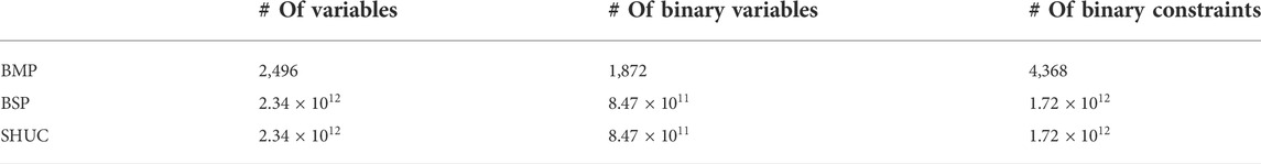
TABLE 4. The problem scale of the BMP, BSP, and SHUC model.

The simulation program was run on a personal computer with an Intel i7-7900K processor, 3.30 GHz, and 16GB RAM. The commercial solver, CPLEX 12.9 under Python environment, was called to solve the model.

4.2 Results

4.2.1 Deterministic case

We first apply our solution method in a deterministic unit commitment model to verify our code. In the deterministic case, the uncertainty of the market price is not considered, i.e., only one price scenario (the forecast price) is input to the unit commitment model. Therefore, the inner layer algorithm is actually a dual dynamic integer programming (DDP) algorithm (Pereira and Pinto, 1991). Therefore, the convergence criterion needs to be modified. Here, the gap between the upper and lower bound ($\epsilon$) is set as the convergence criterion, as shown in (Eq. 44). The convergence tolerance of the DDP algorithm is set as 0.01%.

$\epsilon =\frac{U{B}_{\mathbf{DDP}}-L{B}_{\mathbf{DDP}}}{L{B}_{\mathbf{DDP}}}(44)$

Where $U{B}_{\mathbf{DDP}}$ and $L{B}_{\mathbf{DDP}}$ are the upper and lower bound of the DDP algorithm, respectively.

We apply the CPLEX to solve the deterministic model directly (no decomposition method is used) and compare it with the proposed solution method. The comparison results are shown in Table 5. It can be seen that the relative error between the two methods is less than 0.001%. The solution time of the CPLEX is 8.8 times that of the proposed method, which shows the advantage of the proposed solution method.

TABLE 5

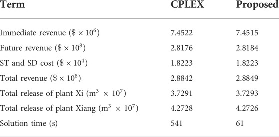
TABLE 5. The comparison of the solution results between CPLEX and the proposed method.

Figure 5 lists the startup and shutdown status of all units in the two plants. Due to the constraints (Eqs 22–25), the number of startup and shutdown and the online/offline time of all units satisfy the pre-set data.

FIGURE 5

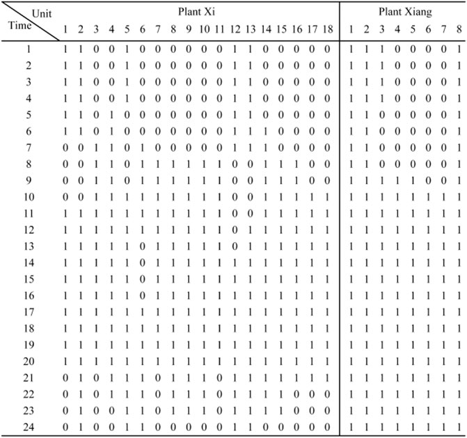
FIGURE 5. The startup and shutdown status of units in the two plants.

Figure 6 shows the 24-hour power generation schedule of two plants. Figure 7 shows the evolution of the reservoir volumes. The termination volumes of the two reservoirs are 68.847e8 m³ and 44.95e8 m³, respectively. During the low price period, the reservoir volume of plant Xi increased by 3.07e6 m³, which indicates that the discharge is less than the inflow. Using the water storage during these periods can lift the water head and improve the power generation efficiency.

FIGURE 6

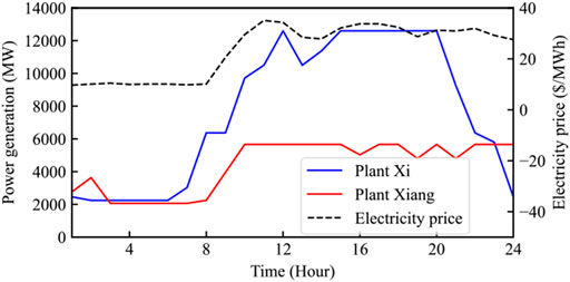
FIGURE 6. The power output of the two plants.

FIGURE 7

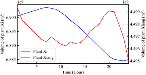
FIGURE 7. The evolution of the reservoir volume of two plants.

4.2.2 Stochastic case

In the stochastic case, the scenario tree generated in Section 4.1 is input to the SHUC model. A set of 500 scenarios is sampled from the complete scenario tree in the forward iteration of the MSDDP algorithm. As in (Pereira and Pinto, 1991), the algorithm stops when the upper bound is within the 95% confidence interval of the lower bound.

The program runs for 2,123 s. Figure 8A shows the upper and lower bounds of the outer layer BD algorithm. The final gap between the upper and lower bounds is 0.0093%. Figure 8B shows the convergence process of the inner layer MSDDP algorithm in the fourth iteration of the BD algorithm. The MSDDP algorithm converges to the 95% confidence interval after 31 iterations.

FIGURE 8

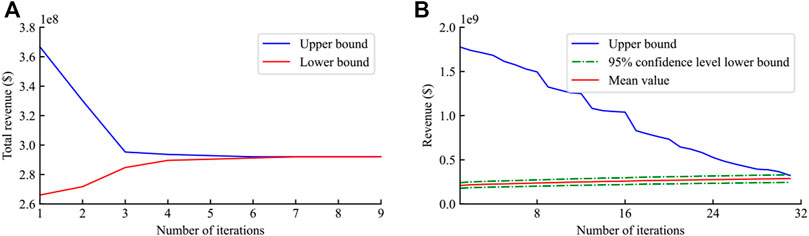
FIGURE 8. The convergence process of the BD algorithm (A) and the MSDDP algorithm in the fourth iteration of the BD algorithm (B).

We then apply the classical Benders Decomposition (CBD) algorithm (Benders, 2005) to solve the SHUC model and compare it with the proposed solution method. The running time is limited to 3 h. The comparison of the solution results is shown in Table 6. The total revenue of the two methods is 2.8036 × 10⁸$ and 2.9204 × 10⁸$, respectively. The revenue of the proposed method is 4% higher than the CBD algorithm. In terms of computational performance, the CBD goes through 25 iterations and finally does not converge to the pre-set tolerance (0.01%). The final gap of the CBD is 3.16%. When using the CBD algorithm to solve the SHUC model, the integer variables must be stored in the master problem, resulting in the loss of effective information related to the optimization direction of the discrete variables. It can only rely on the dual information provided by the subproblem to assist in the optimization of the mater problem. Therefore, more solution time is needed.

TABLE 6

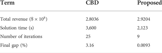
TABLE 6. The comparison of the solution results between CBD and the proposed method.

The value of the stochastic solution (VSS) (Heitsch and Römisch, 2003) is an index used to test the quality of the solution of the stochastic programming problem, as shown in (Eq. 45).

$VSS=RP-EEV(45)$

Where RP represents the optimal value of the stochastic case, which is equal to the weighted average of the objective value of all scenarios. EEV represents the optimal value of the deterministic case.

Compared with the deterministic case, the total revenue of the stochastic case increases by 6.5902 × 10⁶$, accounting for 2.3% of the total revenue. That is, the value of VSS is 6.5902 × 10⁶$. This value represents the cost of ignoring the market price uncertainty in the unit commitment model.

As mentioned in Section 4.1, the termination volumes of the two reservoirs are not set. We end this section by discussing the impact of future revenue constraints (Eq. 14). We set the parameters of the future revenue constraints ${\pi }_{w,k}$ and ${\beta }_w$ to be zero, which enforced the $R^{\text{fut}}$ in the objective function equal to zero. Then the boundary condition (i.e., the termination volumes) should be set in the model to terminate the calculation. The total revenue ratios in different termination volumes to the value in Table 4 (“Proposed”) are shown in Figure 9. It can be seen that the maximum value of the total revenue is equal to the value in Table 6. This indicated that constraints (Eq. 14) could terminate discharging at optimal termination volumes, at which the total revenue of the hydropower producer is maximized. The incorporation of constraints (Eq. 14) in the SHUC model can make a balance between the immediate revenue and the future revenue of the hydropower producer to maximize the total revenue.

FIGURE 9

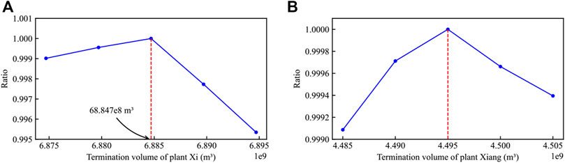
FIGURE 9. The total revenue ratios in different termination volumes to the value in Table 4: (A) the termination volume of plant Xiang is 44.95e8 m³, and (B) the termination volume of plant Xi is 68.847e8 m³.

4.2.3 The impact of the confidence level

Table 7 compares the results of the proposed solution method under different confidence levels. Column 1 represents the final gap of the BD algorithm. The second column represents the iteration number of the BD algorithm. The third column represents the average time used per iteration. Column 4 represents the solution time of the BD algorithm. Finally, column 5 represents the total revenue.

TABLE 7

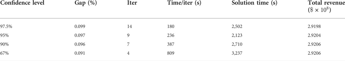
TABLE 7. Comparison of solution results under different confidence levels.

It can be seen that the proposed solution method finally converged under different confidence levels. With the increase of the confidence level, the number of iterations of the BD algorithm decreases while the time used per iteration increases. In fact, the solution obtained in the MSDDP algorithm is getting closer to the optimal solution with the increase in the confidence level. Therefore, the Benders cut provided to the BMP is tighter. While the solution time needed in the MSDDP algorithm also increases. It should be noted that the solution time of the model is shortest when the confidence level is 90%. Therefore, it is necessary to make a trade-off between the solution accuracy of the MSDDP and the number of iterations to minimize the overall solution time. Finally, we can observe that the difference in total revenue under different confidence levels is extremely small. This is because the confidence level is only used to control the convergence of the inner layer MSDDP algorithm. The convergence of the whole algorithm is determined by the gap between the upper and lower bounds of the outer layer BD algorithm. Therefore, the outer layer BMP will adjust the startup and shutdown status of the unit to achieve global optimization.

4.2.4 Computational performance of the MSDDP

In this section, we test the computational performance of the proposed MSDDP algorithm using the data of the hydropower system reported in (Conejo et al., 2002). The hydropower system contains eight plants, with a total capacity of 3,084 MW. The topology and detailed parameters of the hydropower plants are shown in Figure 10 and Table 8, respectively. For the sake of simplicity, the parameters of the future revenue constraints ${\pi }_{w,k}$ and ${\beta }_w$ are set as zero. The initial volume of the reservoirs is shown in Table 9. The termination volumes are equal to the initial volumes. Two alternative methods [Lagrangian relaxation (Steeger and Rebennack, 2017) and locally valid cut (Abgottspon et al., 2014)] are used in the backward iteration of the BSP and compared with the MSDDP algorithm. The confidence level of the three algorithms is set as 90%. Five sets of market price scenarios are sampled in the forward iteration, including 50, 100, 200, 300, and 500 scenarios, respectively. The running time of the programs is limited to 3 h.

FIGURE 10

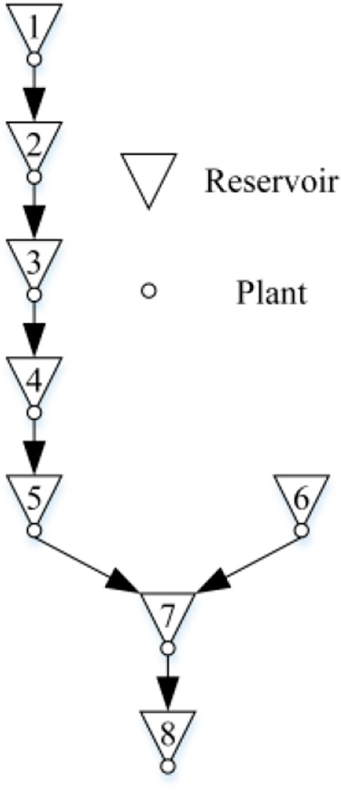
FIGURE 10. The topology of the hydropower system in (Conejo et al., 2002).

TABLE 8

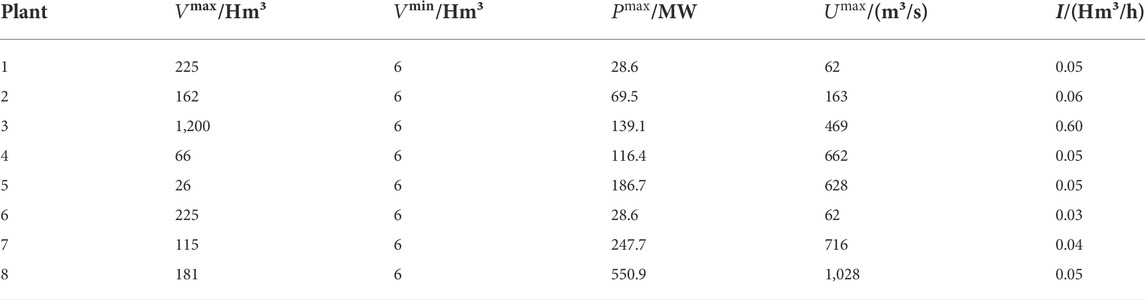
TABLE 8. Technical parameters of the hydropower plants in (Conejo et al., 2002).

TABLE 9

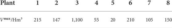
TABLE 9. The initial volume of the reservoirs in (Conejo et al., 2002).

Table 10 shows the comparison of the computational performance of the three algorithms. The first column represents the number of scenarios sampled in the forward iteration. It can be seen that the computation time and the time used per iteration increase with the increase of the forward sample scenarios. This is because more subproblems need to be solved as we increase the number of sample scenarios in the forward iteration. The MSDDP converged to the pre-set tolerance with different choices of the number of the forward sample scenarios. The solution time of the MSDDP algorithm is the shortest among the three algorithms. The LVC and LR method cannot converge to the pre-set tolerance within 3 h when the number of sampled scenarios is 500. It should be noted that the iteration number of the MSDDP algorithm is less than the other two algorithms, which illustrates that the cuts generated by the MSDDP algorithm are the tightest.

TABLE 10

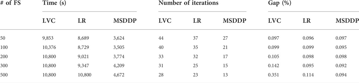
TABLE 10. Computational performance of the locally valid cut (LVC), Lagrangian relaxation (LR) and MSDDP.

5 Conclusion

This paper proposes a stochastic unit commitment model for a price-taker hydropower producer in a liberalized market. The objective is to maximize the total revenue. The opportunity cost and the market price uncertainty are taken into account. To solve the stochastic unit commitment problem efficiently, a solution method based on the Benders decomposition and modified stochastic dual dynamic programming algorithm is proposed. Finally, we verified the effectiveness of the proposed model and solution method in case studies. The simulation results show that: 1) Compared with the deterministic model, the proposed stochastic unit commitment model can increase the total revenue of the hydropower producer by 2.3%, so it is necessary to consider the uncertainty of the market price. 2) The incorporation of future revenue constraints can make a balance between the immediate revenue and the future revenue to maximize the total revenue of the hydropower producer. 3) The proposed solution method can efficiently solve the large-scale stochastic unit commitment problem. Compared with the existing methods, the proposed solution method can significantly reduce the solution time and achieve global optimization.

The following aspects can be further expanded in future research.

1) The proposed SHUC model is actually a two-stage unit commitment model, in which the commitment schedule for the entire scheduling horizon is decided before the uncertainty is realized. The extension of the unit commitment model on the multi-stage model will be promising research.

2) The extension of the modified stochastic dual dynamic programming on the stage-dependent case may be interesting research.

Data availability statement

The original contributions presented in the study are included in the article/Supplementary Material, further inquiries can be directed to the corresponding author.

Author contributions

ZL carried out the formulation of the model, presentation of solution method, case analysis, and wrote the first draft. PY assisted in the formulation of the model and improvement of the solution method. YY and GL assisted in the case analysis. YT helped the revision of the manuscript.

Conflict of interest

The authors declare that the research was conducted in the absence of any commercial or financial relationships that could be construed as a potential conflict of interest.

Publisher’s note

All claims expressed in this article are solely those of the authors and do not necessarily represent those of their affiliated organizations, or those of the publisher, the editors and the reviewers. Any product that may be evaluated in this article, or claim that may be made by its manufacturer, is not guaranteed or endorsed by the publisher.

References

Abgottspon, H., Njálsson, K., Bucher, M. A., and Andersson, G. (2014). “Risk-averse medium-term hydro optimization considering provision of spinning reserves,” in 2014 International Conference on Probabilistic Methods Applied to Power Systems (PMAPS), Durham, UK, 07-10 July 2014 (IEEE).

CrossRef Full Text | Google Scholar

Abreu, L. V. L., Khodayar, M. E., Shahidehpour, M., and Wu, L. (2012). Risk-constrained coordination of cascaded hydro units with variable wind power generation. IEEE Trans. Sustain. Energy 3 (3), 359–368. doi:10.1109/tste.2012.2186322

CrossRef Full Text | Google Scholar

Ackooij, W. V., Ambrosio, C. D., Liberti, L., Taktak, R., Thomopulos, D., and Toubaline, S. (2018). Shortest path problem variants for the hydro unit commitment problem. Electron. Notes Discrete Math. 69, 309–316. doi:10.1016/j.endm.2018.07.040

CrossRef Full Text | Google Scholar

Ackooij, W. V., D'Ambrosio, C., Thomopulos, D., and Trindade, R. S. (2021). Decomposition and shortest path problem formulation for solving the hydro unit commitment and scheduling in a hydro valley. Eur. J. Operational Res. 291 (3), 935–943. doi:10.1016/j.ejor.2020.12.029

CrossRef Full Text | Google Scholar

Ahmed, J. A., and Sarma, A. K. (2005). Genetic algorithm for optimal operating policy of a multipurpose reservoir. Water Resour. Manage. 19 (2), 145–161. doi:10.1007/s11269-005-2704-7

CrossRef Full Text | Google Scholar

Amani, A., and Alizadeh, H. (2021). Solving hydropower unit commitment problem using a novel sequential mixed integer linear programming approach. Water Resour. Manag. 35 (3), 1711–1729. doi:10.1007/s11269-021-02806-6

CrossRef Full Text | Google Scholar

Balas, E., Ceria, S., and CornuéJols, G. (1993). A lift-and-project cutting plane algorithm for mixed 0-1 programs. Math. Program. Ser. A B 58, 295–324. doi:10.1007/BF01581273

CrossRef Full Text | Google Scholar

Balas, E., Ceria, S., and Cornuéjols, G. (1996). Mixed 0-1 programming by lift-and-project in a branch-and-cut framework. Manag. Sci. 42 (9), 1229–1246. doi:10.1287/mnsc.42.9.1229

CrossRef Full Text | Google Scholar

Balas, E. (2011). Disjunctive programming. Pittsburgh, PA: John Wiley & Sons.

Google Scholar

Barroso, L. A. N., Fampa, M. H. C., Kelman, R., Pereira, M. V., and Lino, P. (2002). Market power issues in bid-based hydrothermal dispatch. Ann. Operations Res. 117 (1), 247–270. doi:10.1023/a:1021537910823

CrossRef Full Text | Google Scholar

Benders, J. F. (2005). Partitioning procedures for solving mixed-variables programming problems. Comput. Manag. Sci. 2 (1), 3–19. doi:10.1007/s10287-004-0020-y

CrossRef Full Text | Google Scholar

Birge, J. R., and Louveaux, F. (2011). Introduction to stochastic programming. Chicago, IL: Springer Science & Business Media.

Google Scholar

Cerisola, S., Latorre, J. M., and Ramos, A. (2012). Stochastic dual dynamic programming applied to nonconvex hydrothermal models. Eur. J. Operational Res. 218 (3), 687–697. doi:10.1016/j.ejor.2011.11.040

CrossRef Full Text | Google Scholar

Cheng, C., Wang, J., and Wu, X. (2016). Hydro unit commitment with a head-sensitive reservoir and multiple vibration zones using MILP. IEEE Trans. Power Syst. 31 (6), 4842–4852. doi:10.1109/tpwrs.2016.2522469

CrossRef Full Text | Google Scholar

Colonetti, B., and Finardi, E. C. (2021). Stochastic hydrothermal unit commitment models via stabilized benders decomposition. Electr. Eng. 103 (4), 2197–2211. doi:10.1007/s00202-020-01206-0

CrossRef Full Text | Google Scholar

Conejo, A. J., Arroyo, J. M., Contreras, J., and Villamor, F. (2002). Self-scheduling of a hydro producer in a pool-based electricity market. IEEE Trans. Power Syst. 17 (4), 1265–1272. doi:10.1109/tpwrs.2002.804951

CrossRef Full Text | Google Scholar

Diniz, A. L., and Maceira, M. E. P. (2008). A four-dimensional model of hydro generation for the short-term hydrothermal dispatch problem considering head and spillage effects. IEEE Trans. Power Syst. 23 (3), 1298–1308. doi:10.1109/tpwrs.2008.922253

CrossRef Full Text | Google Scholar

Finardi, E. C., and da Silva, E. L. (2006). Solving the hydro unit commitment problem via dual decomposition and sequential quadratic programming. IEEE Trans. Power Syst. 21 (2), 835–844. doi:10.1109/tpwrs.2006.873121

CrossRef Full Text | Google Scholar

Guisández, I., and Pérez-Díaz, J. I. (2021). Mixed integer linear programming formulations for the hydro production function in a unit-based short-term scheduling problem. Int. J. Electr. Power Energy Syst. 128 (1), 106747. doi:10.1016/j.ijepes.2020.106747

CrossRef Full Text | Google Scholar

Heitsch, H., and Römisch, W. (2003). Scenario reduction algorithms in stochastic programming. Comput. Optim. Appl. 24 (2), 187–206. doi:10.1023/a:1021805924152

CrossRef Full Text | Google Scholar

Helseth, A., Fodstad, M., and Mo, B. (2018). Optimal hydropower maintenance scheduling in liberalized markets. IEEE Trans. Power Syst. 33 (6), 6989–6998. doi:10.1109/tpwrs.2018.2840043

CrossRef Full Text | Google Scholar

Helseth, A., Fodstad, M., and Mo, B. (2016). Optimal medium-term hydropower scheduling considering energy and reserve capacity markets. IEEE Trans. Sustain. Energy 7 (3), 934–942. doi:10.1109/tste.2015.2509447

CrossRef Full Text | Google Scholar

Hjelmeland, M. N., Zou, J., Helseth, A., and Ahmed, S. (2019). Nonconvex medium-term hydropower scheduling by stochastic dual dynamic integer programming. IEEE Trans. Sustain. Energy 10, 481–490. doi:10.1109/TSTE.2018.2805164

CrossRef Full Text | Google Scholar

Kelman, M., Pereira, M., and Campodónico, N. (1998). Long-term hydro scheduling based on stochastic models. EPSOM 98, 23–25.

Google Scholar

Kong, J., Skjelbred, H. I., and Fosso, O. B. (2020). An overview of formulations and optimization methods for the unit-based short-term hydro scheduling problem. Electr. Power Syst. Res. 178, 106027. doi:10.1016/j.epsr.2019.106027

CrossRef Full Text | Google Scholar

Li, X., Li, T., Wei, J., Wang, G., and Yeh, W. W. (2014). Hydro unit commitment via mixed integer linear programming: A case study of the three gorges project, China. IEEE Trans. Power Syst. 29 (3), 1232–1241. doi:10.1109/tpwrs.2013.2288933

CrossRef Full Text | Google Scholar

Lima, R. M., Marcovecchio, M. G., Novais, A. Q., and Grossmann, I. E. (2013). On the computational studies of deterministic global optimization of head dependent short-term hydro scheduling. IEEE Trans. Power Syst. 28 (4), 4336–4347. doi:10.1109/tpwrs.2013.2274559

CrossRef Full Text | Google Scholar

Moiseeva, E., and Hesamzadeh, M. R. (2017). Strategic bidding of a hydropower producer under uncertainty: modified benders approach. IEEE Trans. Power Syst. 33, 861–873. doi:10.1109/TPWRS.2017.2696058

CrossRef Full Text | Google Scholar

Naresh, R., and Sharma, J. (2000). Hydro system scheduling using ANN approach. IEEE Trans. Power Syst. 15 (1), 388–395. doi:10.1109/59.852149

CrossRef Full Text | Google Scholar

Nazari-Heris, M., Mohammadi-Ivatlooa, B., and Gharehpetian, G. B. (2017). Short-term scheduling of hydro-based power plants considering application of heuristic algorithms: A comprehensive review. Renew. Sustain. Energy Rev. 74, 116–129. doi:10.1016/j.rser.2017.02.043

CrossRef Full Text | Google Scholar

Parvez, I., Shen, J., Khan, M., and Cheng, C. (2019). Modeling and solution techniques used for hydro generation scheduling. Water 11 (7), 1392. doi:10.3390/w11071392

CrossRef Full Text | Google Scholar

Peng, L., Zhou, J., Chao, W., Qiao, Q., and Mo, L. (2015). Short-term hydro generation scheduling of Xiluodu and Xiangjiaba cascade hydropower stations using improved binary-real coded bee colony optimization algorithm. Energy Convers. Manag. 91, 19–31. doi:10.1016/j.enconman.2014.11.036

CrossRef Full Text | Google Scholar

Pereira, A. C., de Oliveira, A. Q., Baptista, E. C., Balbo, A. R., Soler, E. M., Nepomuceno, L., et al. (2017). Network-constrained multiperiod auction for pool-based electricity markets of hydrothermal systems. IEEE Trans. Power Syst. 32 (6), 4501–4514. doi:10.1109/tpwrs.2017.2685245

CrossRef Full Text | Google Scholar

Pereira, M., Campodonico, N., and Kelman, R. (1999). Application of stochastic dual DP and extensions to hydrothermal scheduling. PSRI Technical Report 012/99.

Google Scholar

Pereira, M V. F., and Pinto, L M. V. G. (1991). Multi-stage stochastic optimization applied to energy planning. Math. Program. 52 (1), 359–375. doi:10.1007/bf01582895

CrossRef Full Text | Google Scholar

Pérez-Díaz, J. I., Wilhelmi, J. R., and Arévalo, L. A. (2010). Optimal short-term operation schedule of a hydropower plant in a competitive electricity market. Energy Convers. Manag. 51 (12), 2955–2966. doi:10.1016/j.enconman.2010.06.038

CrossRef Full Text | Google Scholar

Seguin, S., Cote, P., and Audet, C. (2016). Self-scheduling short-term unit commitment and loading problem. IEEE Trans. Power Syst. 31 (1), 133–142. doi:10.1109/tpwrs.2014.2383911

CrossRef Full Text | Google Scholar

Shapiro, A. (2011). Analysis of stochastic dual dynamic programming method. Eur. J. Operational Res. 209 (1), 63–72. doi:10.1016/j.ejor.2010.08.007

CrossRef Full Text | Google Scholar

Steeger, G., and Rebennack, S. (2017). Dynamic convexification within nested Benders decomposition using Lagrangian relaxation: an application to the strategic bidding problem. Eur. J. Operational Res. 257 (2), 669–686. doi:10.1016/j.ejor.2016.08.006

CrossRef Full Text | Google Scholar

Thaeer Hammid, A., Awad, O. I., Sulaiman, M. H., Gunasekaran, S. S., Mostafa, S. A., Manoj Kumar, N., et al. (2020). A review of optimization algorithms in solving hydro generation scheduling problems. Energies 13 (11), 2787. doi:10.3390/en13112787

CrossRef Full Text | Google Scholar

Tong, B., Zhai, Q., and Guan, X. (2013). An MILP based formulation for short-term hydro generation scheduling with analysis of the linearization effects on solution feasibility. IEEE Trans. Power Syst. 28 (4), 3588–3599. doi:10.1109/tpwrs.2013.2274286

CrossRef Full Text | Google Scholar

Wei, C., Zhao, Y., Zheng, Y., Xie, L., and Smedley, K. M. (2021). Analysis and design of a nonisolated high step-down converter with coupled inductor and ZVS operation. IEEE Trans. Ind. Electron. 69 (9), 9007–9018. doi:10.1109/tie.2021.3114721

CrossRef Full Text | Google Scholar

Xiao, D., do Prado, J. C., and Qiao, W. (2021). Optimal joint demand and virtual bidding for a strategic retailer in the short-term electricity market. Electr. Power Syst. Res. 190, 106855. doi:10.1016/j.epsr.2020.106855

CrossRef Full Text | Google Scholar

Zhang, H., Zhou, J., Na, F., Zhang, R., and Zhang, Y. (2013). An efficient multi-objective adaptive differential evolution with chaotic neuron network and its application on long-term hydropower operation with considering ecological environment problem. Int. J. Electr. Power Energy Syst. 45 (1), 60–70. doi:10.1016/j.ijepes.2012.08.069

CrossRef Full Text | Google Scholar

Zou, J., Ahmed, S., and Sun, X. A. (2019). Stochastic dual dynamic integer programming. Math. Program. 175 (1), 461–502. doi:10.1007/s10107-018-1249-5

CrossRef Full Text | Google Scholar