 Xinze Xi1
 Xian Wang
- 1Electric Power Research Institute of Yunnan Power Grid Co., Ltd., Kunming, China
- 2Faculty of Mechanical and Electrical Engineering, Kunming University of Science and Technology, Kunming, China
- 3Yunnan International Joint Laboratory of Intelligent Control and Application of Advanced Equipment, Kunming, China
This study proposes an online finite-time adaptive parameter estimation method for grid-connected voltage source inverter (VSI) with LCL filter. In this framework, a time-continuous state-space system model is first developed, which is different from the nonparametric frequency-response-based method. Then, the parameter estimation error information is extracted by introducing a series of filter operations. Moreover, a sliding mode term is studied and cooperated with the obtained parameter estimation error to design the parameter estimation error-based finite-time adaptive parameter estimation algorithm. With the help of this novel adaptive law, the physical parameters of electrical components can be driven to their true values accurately and fast. Theoretical analysis is conducted in terms of the Lyapunov theory to demonstrate the convergence of the parameter estimation error. Finally, numerical simulation results are provided to illustrate the superiority of the proposed method over the conventional method.
1 Introduction
Voltage source inverters (VSIs) are widely implemented in many grid-connected applications due to their capability of converting the DC source to an AC output. In order to convert the current, the inverter is required to implement the pulse modulation technique which will cause high-order harmonic pollution and may trigger a negative impact on grid-connected performance; especially, it may disturb the supply voltage of sensitive loads or devices tied to the grid (Mohamed (2010); Feng et al. (2022)). In order to attenuate the switching frequency harmonics caused by the VSI and improve the quality of the grid capability, a proper filter is needed and implemented between the VSI and the grid practically (Reznik et al. (2013)). Compared with a traditional L-filter (Gomes et al. (2018)), a high-order LCL filter has been generally used in the electrical power system because of its higher attenuation ability and better dynamic characteristics (Tang et al. (2011; 2015)). Moreover, when the range of power levels up to hundreds of kW, the LCL filter can effectively reduce the overall size and weight of the componentswith a small value of inductors and capacitors (Liserre et al. (2005a)).
However, the three-order LCL filter suffers from the resonance problem, which may lead to oscillation of the power grid (Tang et al. (2015)). Although the LCL filter can accommodate the oscillation phenomenon by properly designing the filter parameters (Massing et al. (2011)), some of these parameters may have uncertainties due to the manufacturing tolerances, temperature changes, and the aging of electrical components in practical application. Moreover, if there is a transformer between the filter and the grid, the leakage inductance of the transformer will also lead to uncertainties in the filter (Schlesinger and Biela (2020)), and these lumped uncertainties will impact the overall grid performance.
Since the proper estimation of grid impedance including the LCL filter and VSI has a significant influence on the grid-connected quality, various work based on frequency-response estimation methods (i.e., also known as nonparametric methods) and model-based estimation methods has been done. This kind of method does not assume an exact model and only requires the injected stimulus and the responses. In the work of Liserre et al. (2005b) and Reigosa et al. (2012)), the grid impedance is identified by injecting sinusoidal currents into a grid, in which the Fourier analysis is introduced at a steady state by using the grid-side current and voltage responses. The utilization of sine sweeps provides the highest signal-to-noise ratio (SNR), and thus, it can achieve high-precision identification of the grid impedance. However, this method is not suitable for online identification due to the measurement time and additional power of electronic hardware.
Though frequency-response-based methods are able to describe the dynamic characteristics of the grid, they cannot get the physical parameters of electrical components directly. Furthermore, in many VSI control applications, model-based methods are commonly employed (the controller gains are related as a function of the LCL filter and VSI parameters), such that the prior-knowledge of these uncertain physical parameters is of vital importance. To address the uncertain parameters that existed in electrical power systems, model-based estimation methods are studied in recent years. In (Mohamed and El-Saadany (2008)), the neural networks (NN) based estimation method is proposed, it can obtain great estimation performance, but the NN-based control performance heavily depends on the convergence estimation and rate of NN weights which leads to heavy computational burden. In (Hoffmann and Fuchs (2013)), an extended Kalman filter (EKF) is applied to estimate the electrical components connected in the grid, but the covariance matrices need a tedious parameter tuning procedure.
According to the certainty equivalence principle, the overall performance of the grid will be greatly improved provided that the high accuracy and fast converge rate of online physical parameter estimation in the grid can be obtained. Especially, the start-up performance of the inverter can be simplified and the transient response can be improved. In the traditional adaptive parameter estimation algorithm framework such as the gradient descent method, a predictor and/or observer are generally used to generate predictor and/or observer error to design the adaptive law (de Mathelin and Lozano (1999)). However, the utilization of the gradient descent method may suffer from the potential bursting phenomenon, especially when the system is subject to the external disturbances. In order to overcome this issue, several prevalent robust adaptive laws have been successively proposed such as e-modification (Ioannou and Kokotovic (1983)), and σ-modification (Ortega and Tang (1989)). One salient of such robust adaptive law is that a leakage term is established to ensure the boundedness of the estimated parameters. However, the introduced damping term prevents the estimated parameters from converging to their true values, which means that there is a trade-off between accuracy and boundedness. It is worth noting that the online test of persistent excitation (PE) condition which is used to prove the parameter estimation convergence still remains a difficult challenge in the parameter estimation field. Therefore, it is worthy to further investigate a novel adaptive parameter estimation algorithm, which can not only estimate the system parameter accurately but also provide an intuitive approach to verity the PE condition.
Motivated by the above discussions, this study will propose a novel parameter estimation algorithm for the grid-converter system with LCL filter. To realize this purpose, a series of filter operations and auxiliary variables are used to extract the parameter estimation error information, which is used to construct a novel leakage term and online validate the PE condition. Then, a sliding mode term is studied and cooperated with a new leakage term to design the adaptive finite-time parameter estimation algorithm, by which the system parameters can be driven to their true values accurately and fast. The parameter estimation error convergence is rigorously proved in terms of the Lyapunov theory. Finally, simulation results are provided to demonstrate the effectiveness of the proposed method.
This study is organized as follows. Section 2 provides the dynamic modeling of the grid-connected VSI with LCL filter in continuous-time model. Section 3 presents the finite-time adaptive estimation algorithm design and analysis, and a comparison to another estimation algorithm. Comparison simulations are given in Section 4. Some conclusions are summarized in Section 5.
2 Dynamic modeling
In this section, continuous-time model for grid-connected VSI with LCL filter is first described. As shown in Figure 1, the inverter is supplied with a constant DC voltage udcand an LCL filter is inserted between VSI and the grid to attenuate the switching frequency harmonics caused by VSI. A current controller is applied to regulate the grid-side inductor current and digital control delay Gdelay of the controller is also considered. Moreover, a parameter estimation scheme is added to the system with external disturbances d(t). Note that the aim of this study is to propose a novel parameter estimation scheme to identify the physical parameters of the LCL filter and the digital control delay of VSI with accuracy and fast converge rate.
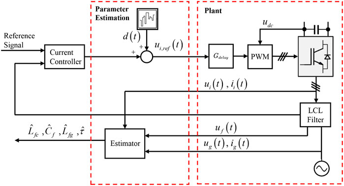
FIGURE 1. Schematic diagram of the estimation setup.
2.1 Model of LCL filter
For the ease of subsequent analysis, a single-phase equivalent circuit model of a typical LCL filter is shown in Figure 2, which is widely used in the grid application. As shown in Figure 2, the symbols ui and ii denote the inverter voltage and inverter current. uf is the voltage across the shunt branch’s filter capacitor, ug and ig represent the grid-side voltage and grid-side current. Li, Lg, and Cf represent the inverter side inductance, the grid-side inductance, and the filter capacitance, respectively. Note that in practical engineering applications, the electrical components such as Li, Lg, and Cf exist uncertainties because of the manufacturing tolerances, temperature changes, and aging phenomenon. Moreover, inductive grid impedance and the leakage inductance caused by the transformer will also lead to the parameter changing of Li and Lg. In order to estimate the physical parameters of electrical components online, the dynamic of the LCL filter can be given by applying the Krichhoff’s law (Massing et al. (2011)), note that equivalent resistors could be ignored since their impedances of them are far less than the one of inductance Li and Lg.
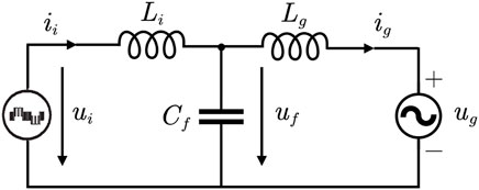
FIGURE 2. Single-phase equivalent circuit diagram.
To facilitate the estimator design, we define the system states as
where
2.2 Model of digitally controlled VSI
The digitally controlled inverters existing time delay includes the computation delay of the microprocessor, sampling period time delay, and time delay of the zero-order hold in the pulse width modulation converter (Agorreta et al. (2010)). Though the three elements are analyzed in the z-domain, few research works focused on the time-domain analysis. In this sense, the following time-continuous model is given:
where τ denotes the sampling period.
Note that Eq. 4 cannot be used to establish the desired state-space form due to its complex transfer function. As analyzed by Agorreta et al. (2010); Houpis (1999); and Houpis and Sheldon (2013), Eq. 4 can be rewritten in terms of the Pade approximation technique as follows:
Based on Eq. 5, a new Gdelay1 can be obtained:
Based on Eq. 2 and 6, the comprehensive state-space form of grid-connected VSI with LCL filter can be formulated as follows:
where
where
ASSUMPTION 1. The system state and the reference control input of the system Eq. 7 are bounded and accessible for measurement.Note that Assumption 1 has been widely used in the estimation field [marino1995adaptive, adetola2008finite], and it can be satisfied by applying a proper controller.
3 Online parameter estimation
In this section, we will propose a finite-time adaptive parameter estimation algorithm to online estimate the unknown parameters encountered in the VSI with LCL filter.
3.1 Finite-time adaptive parameter estimation
For the ease of subsequent analysis, Eq. 7 can be rewritten as
where
where κ > 0 is a positive filter parameter. Note that δf is only used for analysis.
The motivation for adopting the low-pass filter operation can be divided into two aspects. First, the low-pass filter can significantly eliminate the effect of the high-frequency noises (such as measurement noise), which is contributed to improving parameter estimation performance. Second, the measurement of the derivative terms such as
Substituting Eq. 10 into Eq. 9, one can deduce that
It should be pointed out that the non-zero initial condition x (0) may bring an exponentially decaying term
In order to extract the parameter estimation error information with simple algebraic calculation, the auxiliary matrix
where the parameter l > 0 is designed to guarantee the boundness of auxiliary matrix P and vector N. By integrating on both sides of Eq. 12, one can deduce that
Furthermore, another auxiliary vector
where
Generally, the persistent excitation (PE) condition is required to guarantee the parameter estimation convergence in the adaptive parameter estimation. To verify the PE condition online, the following Lemma is given.
Lemma 1:
If the regressor matrix Φ defined in Eq. 9 fulfils the PE condition, the matrix P is positive define, i.e., the minimum eigenvalue of P in Eq. 12 fulfils the condition
Proof: According to the definition of PE (Na et al. (2015)) condition, the inequality
For t > T > 0, Eq. 15 can be rewritten as
Based on Eq. 15 and 16, we can obtain
According to Eq. 17, we can claim that if the matrix P is positive definite, the condition
Remark 1: In order to increase the excitation level, an excitation signal in αβ frame is added to the output of the current loop controller which is also the reference input voltage of inverter uref. The excitation signal is given as un = unα + junβ. We add the excitation signal in β-direction since it can reduce the effects of the inverter nonlinearities on the PWM generator and parameter estimation (Koppinen et al. (2017)). Moreover, the trade-off between excitation power and current harmonic distortion should be carefully considered since a small amplitude of excitation signal will not excite the desired frequency components, while a larger one will cause harmonic distortion in the grid current.
Given the fact that the utilization of parameter estimation error
where Γ1 > 0,
Theorem 1:
For inverter system with LCL filter Eq. 9 and the parameter adaptation law in Eq. 18, the estimation parameter
Proof:
In the inverter system equipped by LCL filter with extra excitation signal, we assume that Φ fulfils the PE condition. And based on Lemma 1, we can guarantee that
where
Focusing on the term
According to Eq. 20 and rewrite it as
Remark 2:
From the above proof, one can find that the convergence rate of estimation error depends on the learning gain Γ1 and excitation level σ. Generally, a large learning gain and excitation level can obtain a faster converge rate, while too large gain may trigger parameter oscillation. The forgetting factor l in Eq. 12 is set to the penalty of the initial condition which is not suggested to be large. Filter parameter κ in Eq. 10 denotes the “bandwidth” of the filter. Hence, there is also a trade-off between converge rate and robustness in selecting the value of the forgetting factor and filter parameter.
3.2 Gradient-based adaptive parameter estimation
In order to further show the superiority of the proposed adaptive law over conventional method, a brief discussion of gradient-based adaptive parameter estimation algorithm is provided in this subsection. First, an observer is designed for the system in Eq. 7:
where λ > 0 denotes the observer gain,
In order to minimize the power of the estimation error e by ∂e2/∂α = 0, one can design the adaptive law by using the observer error e as
where Γ2 denotes the learning gain of gradient-based adaptive law, m2 is a normalizing signal designed by m = 1 + ∥ Φ ∥ as explained by de Mathelin and Lozano (1999). According to Eq. 23, we can find that different from the finite-time estimation algorithm Eq. 18 with parameter estimation error, the gradient-based method depends on a predictor/observer to create the predictor/observer error for driving the adaptive law which may indirect for online parameter estimation.
Remark 3: Grid converters are usually controlled by model-based control algorithms, which means that the estimated parameters like the LCL filter will participate directly/indirectly in the design of the controller. Moreover, from (Xie and Chen (2021); Tao et al. (2022)) we can find that the accuracy and the converge rate of the estimated parameter can impact the overall control performance, which further suggests that a proper estimation algorithm dedicates to grid-connected control. Though there exist some online parameter estimation methods such as gradient-based adaptive law and σ-modification, the estimated parameters may need a fairly time to converge or even not able to converge to the real value. On the contrary, the proposed finite-time adaptive estimation algorithm can drive the estimated parameters toward the real value in finite time. In this sense, the overall control performance can be improved, the controller's overall performance, especially during the start-up period.
4 Simulation
In this section, the parameter estimation of the LCL filter with VSI is simulated in MATLAB/SimPowerSystems software environment. Comparative simulation results are given to demonstrate the effectiveness of the proposed method. The parameters to be estimated and the associate parameters are listed in Table 1 (Koppinen et al. (2017)). Note that the DC voltage is constant and the time delay of digitally control in VSI is considered. Moreover, the sampling frequency is set as fs = 10 kHz and the inverter switching frequency is set at half of the sampling frequency i.e., fPWM = 5 kHz.
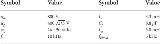
TABLE 1. Simulation system parameters.
The current controller implemented in this simulation is a typical PI controller based on dq synchronous reference frame and the purpose of the controller is to regulate the grid-side inductor current iq. Note that some existing PWM-based control strategies such as repetitive controllers (De Almeida et al. (2014)) and resonant integrator controllers (Yepes et al. (2010)) can be used instead. Moreover, the up-to-date grid-voltage angle ωg can be calculated from the measured grid voltage by the phase-locked loop (PLL) method.
Comparison to gradient-based algorithms: For a fair comparison, the control parameters in the current controller and PLL are taken as the same value, which means that the input signal uref is the same in two estimation process. Moreover, an extra noise
From Figure 3, it can be found that the minimum eigenvalue of matrix P(t) is larger than zero (e.g., λmin (P(t)) > σ > 0). Therefore, the regressor vector Φ satisfies the PE condition according to Lemma 1. Moreover, by calculating the λmin (P(t)), we can online validate the PE condition, which is helpful in practical application. Note that in finite-time estimation, as one can find in previous proof of the theorem, input signals with high excitation levels may improve the convergence rate of estimation errors.
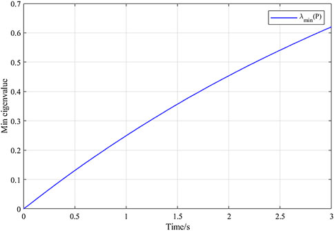
FIGURE 3. Minimum eigenvalue of P(t).
The associated parameters are chosen as
Figure 4 illustrates the comparative parameter estimation performance between the proposed adaptive estimation algorithm and gradient-based estimation algorithm. The estimated parameters based on the aforementioned algorithms are listed in Table 2. As shown in Figure 4 and Table 2, we can find that the proposed adaptive estimation algorithm Eq. 18 obtains a fast parameter convergence speed and accuracy than that of the gradient-based algorithm. The reason for this phenomenon is that the information of parameter estimation error
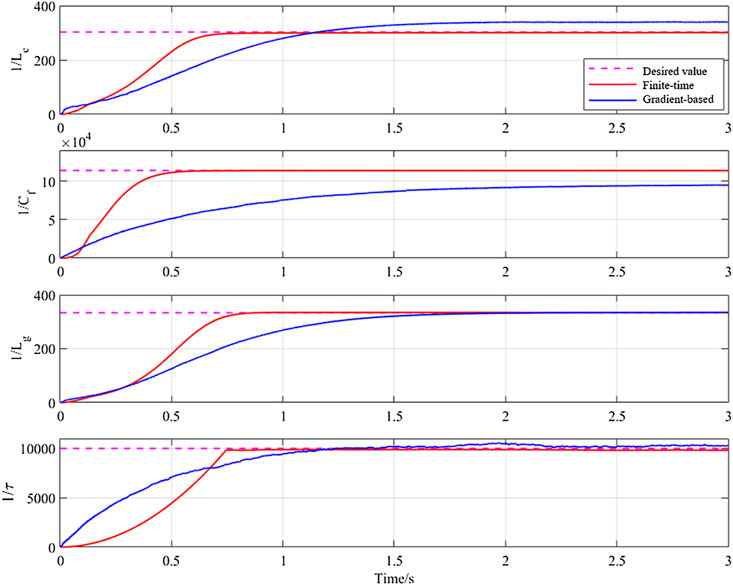
FIGURE 4. Parameter estimation compared with the proposed method and gradient-based method.
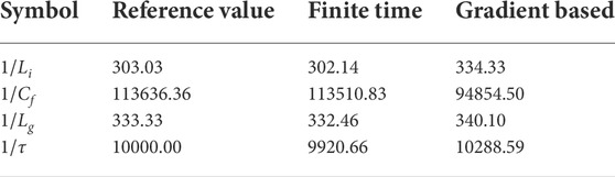
TABLE 2. Estimation of parameters.
Figure 5 provides the frequency responses of the proposed adaptive law and gradient-based adaptive law in terms of the Bode diagram, respectively. We can find from Figure 5 that the proposed adaptive law can accurately estimate the resonant peak and slopes at the high frequency of the LCL filter in the presence of time delay compared with the gradient-based adaptive law due to the precise parameter estimation performance. The improved performance can be also found from the phase angle. Based on the above simulation results, we can further deduce that the proposed parameter estimation method for the LCL filter may provide an alternative way to carry out the corresponding controller design to attenuate the resonant peak to obtain a stable grid current.
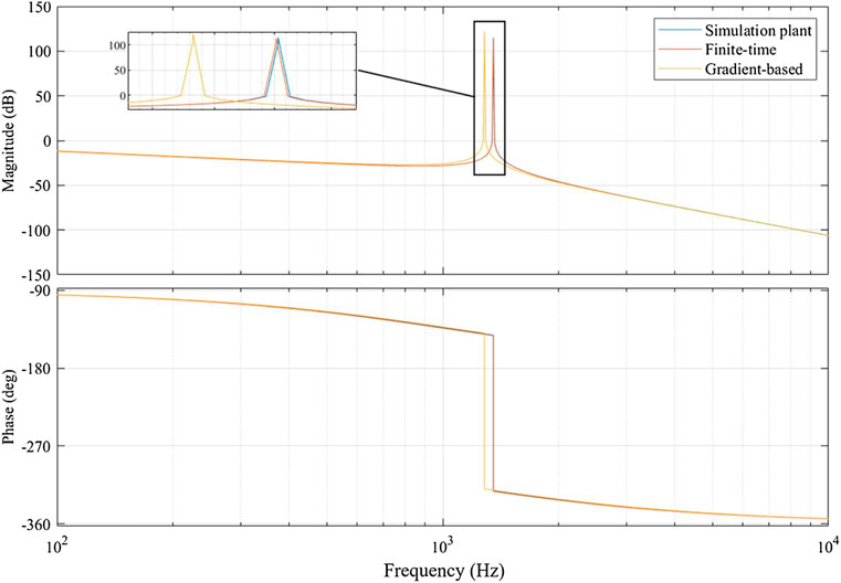
FIGURE 5. Frequency responses of LCL filter with two estimation methods.
5 Conclusion
In this study, an online finite-time adaptive parameter estimation method was proposed for a grid-converter system with LCL filter in time-continuous state-space form. Different from the conventional predictor/observer-based method, the proposed framework could achieve high accuracy and fast converge rate by applying parameter estimation error in driving adaptive law and a sliding mode term is studied and cooperated with new leakage term to design the finite-time adaptive parameter estimation algorithm. Theoretical analysis was studied by Lyapunov theory to demonstrate the convergence of the estimation error. Moreover, a comparative simulation was developed to illustrate the effectiveness of the proposed method. Applying the proposed method to estimate the electrical components can be beneficial for fault diagnosis of the electrical power system. The future work will focus on combining the proposed parameter estimation method with a certain controller to enhance the overall control performance of the grid, and experiments will also carry out in the future.
Data availability statement
The original contributions presented in the study are included in the article/Supplementary Material; further inquiries can be directed to the corresponding author.
Author contributions
XX: analysis, modeling, and writing—original draft. ZS: data curation and writing—original draft. XW: conceptualization and methodology. CX: writing—reviewing the draft. SL: writing—reviewing and editing.
Funding
This work was supported in part by the National Natural Science Foundation of China under Grant 52167011; in part by the National Key Research and Development Program of China under Grant 2019YFE0118000; and in part by the Yunan Fundamental Research Projects under Grant 202001AU070056.
Conflict of interest
XX, CX, and SL were employed by the Electric Power Research Institute of Yunnan Power Grid Co., Ltd.
The remaining authors declare that the research was conducted in the absence of any commercial or financial relationships that could be construed as a potential conflict of interest.
Publisher’s note
All claims expressed in this article are solely those of the authors and do not necessarily represent those of their affiliated organizations, or those of the publisher, the editors, and the reviewers. Any product that may be evaluated in this article, or claim that may be made by its manufacturer, is not guaranteed or endorsed by the publisher.
References
Agorreta, J. L., Borrega, M., López, J., and Marroyo, L. (2010). Modeling and control of N-paralleled grid-connected inverters with LCL filter coupled due to grid impedance in PV plants. IEEE Trans. Power Electron. 26, 770–785. doi:10.1109/TPEL.2010.2095429
Aranovskiy, S., Bobtsov, A. A., Pyrkin, A. A., Ortega, R., and Chaillet, A. (2015). Flux and position observer of permanent magnet synchronous motors with relaxed persistency of excitation Conditions∗∗This article is supported by government of Russian federation (grant 074-U01, GOSZADANIE 2014/190 (project 2118)), the ministry of education and science of Russian federation (project 14.Z50.31.0031). IFAC-PapersOnLine 48, 301–306. doi:10.1016/j.ifacol.2015.09.202
Aranovskiy, S., Bobtsov, A., Ortega, R., and Pyrkin, A. (2016). “Parameters estimation via dynamic regressor extension and mixing,” in 2016 American Control Conference (ACC) (Boston, MA, USA: IEEE), 6971–6976. doi:10.1109/ACC.2016.7526771
De Almeida, P. M., Duarte, J. L., Ribeiro, P. F., and Barbosa, P. G. (2014). Repetitive controller for improving grid-connected photovoltaic systems. IET Power Electron. 7, 1466–1474. doi:10.1049/iet-pel.2013.0546
de Mathelin, M., and Lozano, R. (1999). Robust adaptive identification of slowly time-varying parameters with bounded disturbances. Automatica 35, 1291–1305. doi:10.1016/S0005-1098(99)00026-6
Feng, C., Liang, B., Li, Z., Liu, W., and Wen, F. (2022). Peer-to-peer energy trading under network constraints based on generalized fast dual ascent. IEEE Trans. Smart Grid 1, 3162876. doi:10.1109/tsg.2022.3162876
Gomes, C. C., Cupertino, A. F., and Pereira, H. A. (2018). Damping techniques for grid-connected voltage source converters based on lcl filter: An overview. Renew. Sustain. Energy Rev. 81, 116–135. doi:10.1016/j.rser.2017.07.050
Hoffmann, N., and Fuchs, F. W. (2013). Minimal invasive equivalent grid impedance estimation in inductive–resistive power networks using extended kalman filter. IEEE Trans. Power Electron. 29, 631–641. doi:10.1109/TPEL.2013.2259507
Houpis, C. H. (1999). Quantitative feedback theory: Fundamentals and applications. Boca Raton, FL, USA: CRC Press. doi:10.4324/9780203908051
Houpis, C. H., and Sheldon, S. N. (2013). Linear control system Analysis and design with MATLAB®. Boca Raton, FL, USA: CRC Press.
Ioannou, P. A., and Kokotovic, P. V. (1983). Adaptive systems with reduced models. Berlin, Germany: Springer. doi:10.1007/BFb0006363
Koppinen, J., Kukkola, J., and Hinkkanen, M. (2017). Plug-in identification method for an lcl filter of a grid converter. IEEE Trans. Ind. Electron. 65, 6270–6280. doi:10.1109/TIE.2017.2787546
Liserre, M., Blaabjerg, F., and Hansen, S. (2005a). Design and control of an lcl-filter-based three-phase active rectifier. IEEE Trans. Ind. Appl. 41, 1281–1291. doi:10.1109/TIA.2005.853373
Liserre, M., Blaagjerg, F., and Teodorescu, R. (2005b). “Grid impedance detection via excitation of lcl-filter resonance,” in Fourtieth IAS Annual Meeting. Conference Record of the 2005 Industry Applications Conference, 2005 (Hong Kong, China: IEEE), 910–916. Vol. 2.
Massing, J. R., Stefanello, M., Grundling, H. A., and Pinheiro, H. (2011). Adaptive current control for grid-connected converters with lcl filter. IEEE Trans. Ind. Electron. 59, 4681–4693. doi:10.1109/TIE.2011.2177610
Mohamed, Y. A.-R. I., and El-Saadany, E. F. (2008). Adaptive discrete-time grid-voltage sensorless interfacing scheme for grid-connected dg-inverters based on neural-network identification and deadbeat current regulation. IEEE Trans. Power Electron. 23, 308–321. doi:10.1109/TPEL.2007.911879
Mohamed, Y. A.-R. I. (2010). Mitigation of dynamic, unbalanced, and harmonic voltage disturbances using grid-connected inverters with $LCL$ filter. IEEE Trans. Ind. Electron. 58, 3914–3924. doi:10.1109/TIE.2010.2098372
Na, J., Mahyuddin, M. N., Herrmann, G., Ren, X., and Barber, P. (2015). Robust adaptive finite-time parameter estimation and control for robotic systems. Int. J. Robust Nonlinear Control 25, 3045–3071. doi:10.1002/rnc.3247
Na, J., Wang, S., Liu, Y.-J., Huang, Y., and Ren, X. (2019). Finite-time convergence adaptive neural network control for nonlinear servo systems. IEEE Trans. Cybern. 50, 2568–2579. doi:10.1109/TCYB.2019.2893317
Ortega, R., Praly, L., Aranovskiy, S., Yi, B., and Zhang, W. (2018). On dynamic regressor extension and mixing parameter estimators: Two luenberger observers interpretations. Automatica 95, 548–551. doi:10.1016/j.automatica.2018.06.011
Ortega, R., and Tang, Y. (1989). Robustness of adaptive controllers — A survey. Automatica 25, 651–677. doi:10.1016/0005-1098(89)90023-X
Reigosa, D., Briz, F., Charro, C. B., García, P., and Guerrero, J. M. (2012). Active islanding detection using high-frequency signal injection. IEEE Trans. Ind. Appl. 48, 1588–1597. doi:10.1109/TIA.2012.2209190
Reznik, A., Simões, M. G., Al-Durra, A., and Muyeen, S. (2013). $LCL$ filter design and performance analysis for grid-interconnected systems. IEEE Trans. Ind. Appl. 50, 1225–1232. doi:10.1109/TIA.2013.2274612
Schlesinger, R., and Biela, J. (2020). Comparison of analytical models of transformer leakage inductance: Accuracy versus computational effort. IEEE Trans. Power Electron. 36, 146–156. doi:10.1109/TPEL.2020.3001056
Tang, Y., Loh, P. C., Wang, P., Choo, F. H., and Gao, F. (2011). Exploring inherent damping characteristic of lcl-filters for three-phase grid-connected voltage source inverters. IEEE Trans. Power Electron. 27, 1433–1443. doi:10.1109/TPEL.2011.2162342
Tang, Y., Yao, W., Loh, P. C., and Blaabjerg, F. (2015). Design of lcl filters with lcl resonance frequencies beyond the nyquist frequency for grid-connected converters. IEEE J. Emerg. Sel. Top. Power Electron. 4, 3–14. doi:10.1109/JESTPE.2015.2455042
Tao, M., Chen, Q., He, X., and Xie, S. (2022). Fixed-time filtered adaptive parameter estimation and attitude control for quadrotor uavs. IEEE Trans. Aerosp. Electron. Syst. 1, 3159770. doi:10.1109/TAES.2022.3159770
Xie, S., and Chen, Q. (2021). Adaptive nonsingular predefined-time control for attitude stabilization of rigid spacecrafts. IEEE Trans. Circuits Syst. Ii. 69, 189–193. doi:10.1109/TCSII.2021.3078708
Keywords: adaptive parameter estimation, finite-time convergence, LCL filters, voltage source inverters, parameter identification
Citation: Xi X, Shi Z, Wang X, Xing C and Li S (2022) Adaptive finite-time parameter estimation for grid-connected converter with LCL filter. Front. Energy Res. 10:964216. doi: 10.3389/fenrg.2022.964216
Received: 08 June 2022; Accepted: 12 July 2022;
Published: 05 September 2022.
Edited by:
Changsen Feng, Zhejiang University of Technology, ChinaReviewed by:
Shubo Wang, Qingdao University, ChinaZhijing Liao, Queen Mary University of London, United Kingdom
Yongfeng Lyu, University of Warwick, United Kingdom
Copyright © 2022 Xi, Shi, Wang, Xing and Li. This is an open-access article distributed under the terms of the Creative Commons Attribution License (CC BY). The use, distribution or reproduction in other forums is permitted, provided the original author(s) and the copyright owner(s) are credited and that the original publication in this journal is cited, in accordance with accepted academic practice. No use, distribution or reproduction is permitted which does not comply with these terms.
*Correspondence: Xian Wang, d2FuZ2x5d3hpYW5AMTYzLmNvbQ==