 Yuan Du1
 Yixun Xue
- 1College of Electrical and Power Engineering, Taiyuan University of Technology, Taiyuan, China
- 2Hangzhou Dianzi University Information Engineering College, Hangzhou, China
- 3Guodian Nanjing Automation Co., Ltd., Nanjing, China
- 4State Grid Zhejiang Electric Power Research Institute, Hangzhou, China
With the wide deployment of combined heat and power units, electric boilers, etc., the power system and the heating system are coupled tightly, which necessitates expansion planning in a coordinated manner. Demand response (DR) is considered an effective method for augmenting system flexibility, which would lead to a more beneficial planning strategy in the co-expansion planning strategy. Therefore, we develop a bi-level co-expansion planning model with DR constraints for the integrated electric and heating system to minimize expenses on both investment and operation. The upper level gives the optimal investment strategy of energy facilities, while the lower level is optimal operation problems with DR constraints under the given investment decision. Numerical simulation is employed in the P6H8 system to demonstrate the proposed model.
1 Introduction
The widespread deployment of combined heat and power (CHP) units augments the interconnection between the power system and the heating system (Lin et al., 2020; Khatibi et al., 2021). In this context, the integrated electric and heating system (IEHS) has gained massive attention in recent years. IEHS is an important part of the Energy Internet (Long et al., 2022), and it has received extensive attention in both industry and academia.
Extensive studies on the optimal operation of IEHS can be found in the literature. Li et al. (2016) proposed a combined heat and power dispatch (CHPD) method that exploits the flexibility of the district heating system (DHS) for better wind accommodation in the power system. And Xue et al. (2020) developed a heterogeneous decomposition algorithm to tackle the multi-agent problem in CHPD. In addition to economic dispatch, other operation problems such as unit commitment (Anand et al., 2019) and optimal energy flow (Yao et al., 2021) are also studied.
The aforementioned studies are based on given energy facilities which may not provide sufficient operation flexibility once the load increases (Fu et al., 2020). On this account, the co-expansion planning (CEP) of IEHS is another research priority. Li et al. (2021) proposed a CEP method for hybrid concentrating solar power and CHP plant in IEHS. Cheng et al. (2019) developed a CEP model aimed at minimizing cost and emissions. Martinez Cesena et al. (2016) proposed a CEP model for IEHS to address long-term price uncertainty. Cao et al. (2020) proposed a data-driven method to solve the CEP with uncertainty.
However, the aforementioned studies usually formulate the CEP problem as a single-layer model, which is unreasonable. In industry practice, the investment and operation are determined by the generation company and system operator, respectively (Pineda and Morales, 2019). The generation company determines the investment strategy, which is submitted to the system operator. And the system operator develops a cost-effective operation strategy, which regulates the unit operation. Thus, it is urgent to develop a CEP framework to capture this feature.
Considering the impact of the operation strategies on investment decisions, fully exploiting flexibility resources in IEHS operation will result in more beneficial planning strategies. Demand response (DR) is an important way to mobilize flexible resources on the demand side (Huang et al., 2019; Gjorgievski et al., 2021), which has been studied extensively in quantitative evaluation (D’hulst et al., 2015), economic dispatch (Alipour et al., 2019; Majidi et al., 2019) and unit commitment (Mansour-Saatloo et al., 2020). In contrast, few works focus on the performance of DR on CEP problems. DR could optimize the load curves by intentionally modifying the energy consumption patterns of users to facilitate IEHS in balancing supply and demand (Yin et al., 2016). Thus, DR can be regarded as a potential tool to postpone or even cancel unnecessary facilities planning.
Accordingly, the focus of this paper is to develop a bi-level co-expansion planning (BLCEP) model with DR constraints for IEHS. The main contributions of our work are as follows:
1) We develop a BLCEP framework of IEHS in this paper. The investment of power and heat sources are optimized in the upper level, while the operation problem is optimized in the lower level. In this way, the optimal results can be obtained through the game of the upper-level problem and the lower-level problem.
2) DR is introduced into the BLCEP model, and its cost is considered in the objective function. The electric and heat load curve is optimized by DR, and the operation flexibility of the demand side is exploited. In this way, unnecessary investment in IEHS facilities is prevented.
3) The proposed BLCEP model is transformed into a single-layer model by replacing the lower-level operation model with corresponding Karush-Kuhn-Tucker (KKT) conditions. Therefore, the proposed model can be solved directly with commercial solvers such as CPLEX and Gurobi.
The remainder of this paper is as follows. In Section 2, we proposed a BLCEP framework of IEHS. Based on the framework, a BLCEP model with DR constraints is given in Section 3. In Section 4, the proposed BLCEP model is transformed into a single-level mixed integer linear optimization problem. In Section 5, numerical simulations of the P6H8 system are performed to demonstrate the effectiveness of the proposed model. And the conclusion is given in Section 6.
2 Framework
A typical IEHS is comprised of an electric power system (EPS) and DHSs. In this regard, the expansion planning for IEHS includes planning for both power and heat sources. Figure 1 depicts the BLCEP framework of IEHS. An investment model is presented in the upper level, which is utilized to determine the optimal investment strategy for energy facilities. Based on the investment decision given by the upper level, the IEHS operation problem is optimized to minimize the operation costs at the lower level and feedback to the upper level.
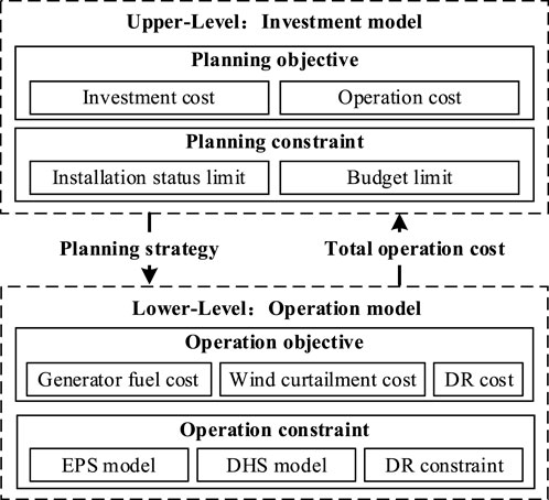
FIGURE 1. Framework of BLCEP of IEHS problem.
Noting that the investment model in the upper level and the operation model in the lower level are mutually influenced. The less investment in expansion, the stricter operation conditions, and the larger operation cost. Similarly, lower operation costs require more relaxed operation conditions, i.e., more investment in energy facilities. Hence, the optimal solution of bi-level programming can be regarded as the gaming between the investment level and operation level (Zeng et al., 2017; Wang et al., 2021).
3 Bi-level co-expansion planning of integrated electric and heating system model formulation
Based on the framework given in Section 2, the BLCEP model is formulated as follows.
3.1 Investment model in the upper level
Denote
The first term indicates the investment cost of energy facilities which consist of generators, wind farms and electric boilers, i.e.,
where dr indicates the discount rate, and it generally takes a value between 6% and 8% (Mu et al., 2020). The second term of (1) indicates operation cost in
The upper-level model is subjected to investment constraints. 1) duplicate investment of energy facilities is prohibited (4)–(6). 2) annual investment cost is limited by budget (7).
where
3.2 Operation model in the lower level
The objective function
where
where
In addition to the objective, operation constraints of DHS and EPS would have to be considered in the model as follows.
3.2.1 District heating system operation constraints
Generally, heat is generated by heating facilities such as CHP units, electric boilers in heat stations, i.e.,
where
As for electric boilers, they can be formulated as
where
where
Let
where
According to the energy conservation, the temperatures of mass flow rate would mix when mass flow into the same heat node, i.e.,
where
Considering heating dissipation during heating transfer, the outlet temperature of mass flow rate in pipelines is lower than the inlet temperature.
where
3.1.2 Electric power system operation constraints
Let
where
3.2.3 Demand response constraints
The demand response is considered in this paper. Denote
To guarantee user satisfaction, the total amount of load in the subperiod
where
4 Solving strategy
For brevity, the BLCEP model proposed in Section 3 is rewritten in matrix form, as follows
where
Since the lower-level operation problem with fixed investment decision is linear, it can be replaced by corresponding KKT conditions as follows:
In (38), the non-linear constraint
where
5 Case study
In this section, a modified P6H8 system is utilized to testify the proposed model. The modified P6H8 system is shown in Figure 2, which comprised a six-buses electric power system and an eight-nodes district heating system. The planning horizon is 10 years, while each year is divided into three typical days (transition season, summer, and winter) with hourly timesteps. The candidate facilities data is presented in Table 1. The annual growth rate of the power load is 2.5%, and that of the heat load is 4%. The discount rate is 8%. The load change rate
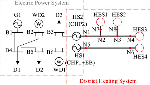
FIGURE 2. A modified P6H8 system.
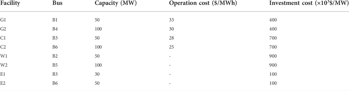
TABLE 1. Candidate facilities data.
To compare and analyze the proposed model, two cases are employed as follows:
Case 1: Determine the planning strategy of IEHS using the BLCEP method without DR.
Case 2: Determine the planning strategy of IEHS using the BLCEP method with DR constraints developed in this paper.
All the test is performed on 11th Gen Intel(R) Core (TM) i7-1165G7 at 2.80GHz CPU, 16GB RAM system. The proposed BLCEP model is coded using Matlab R2020a with Gurobi 9.5.0 Solver.
5.1 Case 1
In Case 1, the IEHS is planned and operated in a coordinated mode without demand response. The installation year of candidate facilities is presented in Table 2, and the co-planning cost is presented in Table 3. During the whole planning horizon, five facilities (i.e., G1, G2, C1, W1, and E1) would have to be installed to satisfy increased loads at a total cost of $ 1.37×10⁸.
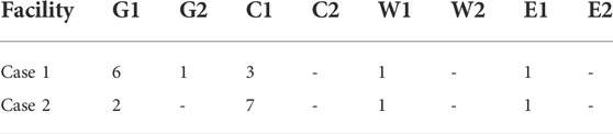
TABLE 2. Installation year of candidate facilities.

TABLE 3. Cost comparison between Case 1 and 2.
5.2 Case 2
We consider a BLCEP method that considers demand response in Case 2. As shown in Figure 3, the peak power loads in the first summer and winter are transferred to valley periods by DR to facilitate the supply-demand balance of power. Due to the tight coupling of power and heat, valley heat loads can be shifted to peak periods in summer for dispatching CHP units to supply peak power loads. Hence, G2 is canceled, as shown in Table 2. As shown in Figure 4. the peak heat loads in the third winter are transferred to valley periods by DR to facilitate the supply-demand balance of heat, so that C1 is postponed.
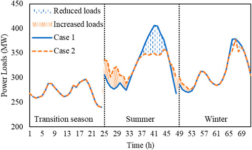
FIGURE 3. Power loads curves in the first year.
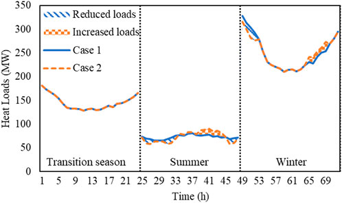
FIGURE 4. Heat loads curves in the third year.
As shown in Table 2, Case 2 cancels G2 installation and postpones C1 installation in comparison to Case 1. Hence, the investment cost could be reduced by $ 0.43 × 10⁸ even if G1 is installed ahead. Considering the shifted loads would like to be supplied by cost-effective units, the generator fuel cost is reduced by $ 0.13 × 10⁸. Besides, wind curtailment costs are reduced by $ 2.02 × 10⁶ by exploiting the flexibility of loads to consume wind power. As a result, the total cost is reduced by $ 0.44 × 10⁸.
6 Conclusion
The proposed BLCEP framework achieves the game optimization of investment and operation, which can be utilized in CEP in other systems. DR is introduced in the BLCEP model and analyzed in the case study. It is found that DR would help the generation company with decision support to develop a more beneficial planning strategy.
The BLCEP model proposed in this paper is oriented to deterministic scenarios. However, intermittent renewable power outputs and variable load demands will bring challenges to IEHS economic and safe operation (Fu, 2022), ultimately affecting planning strategies. In our future works, the uncertainty of renewable power and load demands will be considered in our model.
Data availability statement
The datasets presented in this study can be found in online repositories. The names of the repository/repositories and accession number(s) can be found below: https://docs.google.com/spreadsheets/d/13TcFGtE5cLdSJiCrPx0PsfU3gLrKAqE4/edit?usp=sharing&ouid=115924522171410221124&rtpof=true&sd=true.
Author contributions
YD: Conceptualization, Methodology, Formal Analysis, Writing-Original Draft YX: Conceptualization, Supervision, Writing-Reviewing and Editing LL: Writing- Validation, Reviewing and Editing CY: Visualization JZ: Validation.
Conflict of interest
CY was employed by Guodian Nanjing Automation Co., Ltd.
The remaining authors declare that the research was conducted in the absence of any commercial or financial relationships that could be construed as a potential conflict of interest.
Publisher’s note
All claims expressed in this article are solely those of the authors and do not necessarily represent those of their affiliated organizations, or those of the publisher, the editors and the reviewers. Any product that may be evaluated in this article, or claim that may be made by its manufacturer, is not guaranteed or endorsed by the publisher.
References
Alipour, M., Zare, K., Seyedi, H., and Jalali, M. (2019). Real-time price-based demand response model for combined heat and power systems. Energy 168, 1119–1127. doi:10.1016/j.energy.2018.11.150
Anand, H., Narang, N., and Dhillon, J. S. (2019). Multi-objective combined heat and power unit commitment using particle swarm optimization. Energy 172, 794–807. doi:10.1016/j.energy.2019.01.155
Cao, Y., Wei, W., Wang, J., Mei, S., Shafie-khah, M., and Catalao, J. P. S. (2020). Capacity planning of energy hub in multi-carrier energy networks: A data-driven robust stochastic programming approach. IEEE Trans. Sustain. Energy 11, 3–14. doi:10.1109/TSTE.2018.2878230
Cheng, Y., Zhang, N., Lu, Z., and Kang, C. (2019). Planning multiple energy systems toward low-carbon society: A decentralized approach. IEEE Trans. Smart Grid 10, 4859–4869. doi:10.1109/TSG.2018.2870323
D’hulst, R., Labeeuw, W., Beusen, B., Claessens, S., Deconinck, G., and Vanthournout, K. (2015). Demand response flexibility and flexibility potential of residential smart appliances: Experiences from large pilot test in Belgium. Appl. Energy 155, 79–90. doi:10.1016/j.apenergy.2015.05.101
Fu, X., Guo, Q., and Sun, H. (2020). Statistical machine learning model for stochastic optimal planning of distribution networks considering a dynamic correlation and dimension reduction. IEEE Trans. Smart Grid 11, 2904–2917. doi:10.1109/TSG.2020.2974021
Fu, X. (2022). Statistical machine learning model for capacitor planning considering uncertainties in photovoltaic power. Prot. Control Mod. Power Syst. 7, 5. doi:10.1186/s41601-022-00228-z
Gjorgievski, V. Z., Markovska, N., Abazi, A., and Duić, N. (2021). The potential of power-to-heat demand response to improve the flexibility of the energy system: An empirical review. Renew. Sustain. Energy Rev. 138, 110489. doi:10.1016/j.rser.2020.110489
Huang, W., Zhang, N., Kang, C., Li, M., and Huo, M. (2019). From demand response to integrated demand response: Review and prospect of research and application. Prot. Control Mod. Power Syst. 4, 12. doi:10.1186/s41601-019-0126-4
Khatibi, M., Bendtsen, J. D., Stoustrup, J., and Molbak, T. (2021). Exploiting power-to-heat assets in district heating networks to regulate electric power network. IEEE Trans. Smart Grid 12, 2048–2059. doi:10.1109/TSG.2020.3044348
Li, X., Wu, X., Gui, D., Hua, Y., and Guo, P. (2021). Power system planning based on CSP-CHP system to integrate variable renewable energy. Energy 232, 121064. doi:10.1016/j.energy.2021.121064
Li, Z., Wu, W., Shahidehpour, M., Wang, J., and Zhang, B. (2016). Combined heat and power dispatch considering pipeline energy storage of district heating network. IEEE Trans. Sustain. Energy 7, 12–22. doi:10.1109/TSTE.2015.2467383
Lin, C., Wu, W., Wang, B., Shahidehpour, M., and Zhang, B. (2020). Joint commitment of generation units and heat exchange stations for combined heat and power systems. IEEE Trans. Sustain. Energy 11, 1118–1127. doi:10.1109/TSTE.2019.2917603
Long, H., Fu, X., Kong, W., Chen, H., Zhou, Y., and Yang, F. (2022). Key technologies and applications of rural energy internet in China. Inf. Process. Agric. doi:10.1016/j.inpa.2022.03.001
Majidi, M., Mohammadi-Ivatloo, B., and Anvari-Moghaddam, A. (2019). Optimal robust operation of combined heat and power systems with demand response programs. Appl. Therm. Eng. 149, 1359–1369. doi:10.1016/j.applthermaleng.2018.12.088
Mansour-Saatloo, A., Agabalaye-Rahvar, M., Mirzaei, M. A., Mohammadi-Ivatloo, B., Abapour, M., and Zare, K. (2020). Robust scheduling of hydrogen based smart micro energy hub with integrated demand response. J. Clean. Prod. 267, 122041. doi:10.1016/j.jclepro.2020.122041
Martinez Cesena, E. A., Capuder, T., and Mancarella, P. (2016). Flexible distributed multienergy generation system expansion planning under uncertainty. IEEE Trans. Smart Grid 7, 348–357. doi:10.1109/TSG.2015.2411392
Mu, Y., Chen, W., Yu, X., Jia, H., Hou, K., Wang, C., et al. (2020). A double-layer planning method for integrated community energy systems with varying energy conversion efficiencies. Appl. Energy 279, 115700. doi:10.1016/j.apenergy.2020.115700
Pineda, S., and Morales, J. M. (2019). Solving linear bilevel problems using big-Ms: Not all that glitters is gold. IEEE Trans. Power Syst. 34, 2469–2471. doi:10.1109/TPWRS.2019.2892607
Shao, C., Shahidehpour, M., and Ding, Y. (2020). Market-based integrated generation expansion planning of electric power system and district heating systems. IEEE Trans. Sustain. Energy 11, 2483–2493. doi:10.1109/TSTE.2019.2962756
Wang, D., Zhi, Y., Jia, H., Hou, K., Zhang, S., Du, W., et al. (2019). Optimal scheduling strategy of district integrated heat and power system with wind power and multiple energy stations considering thermal inertia of buildings under different heating regulation modes. Appl. Energy 240, 341–358. doi:10.1016/j.apenergy.2019.01.199
Wang, L., Zhu, Z., Jiang, C., and Li, Z. (2021). Bi-level robust optimization for distribution system with multiple microgrids considering uncertainty distribution locational marginal price. IEEE Trans. Smart Grid 12, 1104–1117. doi:10.1109/TSG.2020.3037556
Xue, Y., Li, Z., Lin, C., Guo, Q., and Sun, H. (2020). Coordinated dispatch of integrated electric and district heating systems using heterogeneous decomposition. IEEE Trans. Sustain. Energy 11, 1495–1507. doi:10.1109/TSTE.2019.2929183
Yao, S., Gu, W., Lu, S., Zhou, S., Wu, Z., Pan, G., et al. (2021). Dynamic optimal energy flow in the heat and electricity integrated energy system. IEEE Trans. Sustain. Energy 12, 179–190. doi:10.1109/TSTE.2020.2988682
Yin, R., Kara, E. C., Li, Y., DeForest, N., Wang, K., Yong, T., et al. (2016). Quantifying flexibility of commercial and residential loads for demand response using setpoint changes. Appl. Energy 177, 149–164. doi:10.1016/j.apenergy.2016.05.090
Keywords: co-expansion planning, integrated electric and heating system, district heating system, bi-level programming, demand response
Citation: Du Y, Xue Y, Lu L, Yu C and Zhang J (2022) A bi-level co-expansion planning of integrated electric and heating system considering demand response. Front. Energy Res. 10:999948. doi: 10.3389/fenrg.2022.999948
Received: 21 July 2022; Accepted: 19 August 2022;
Published: 27 September 2022.
Edited by:
Xueqian Fu, China Agricultural University, ChinaReviewed by:
Lingling Wang, Shanghai Jiao Tong University, ChinaBo Liu, Kansas State University, United States
Copyright © 2022 Du, Xue, Lu, Yu and Zhang. This is an open-access article distributed under the terms of the Creative Commons Attribution License (CC BY). The use, distribution or reproduction in other forums is permitted, provided the original author(s) and the copyright owner(s) are credited and that the original publication in this journal is cited, in accordance with accepted academic practice. No use, distribution or reproduction is permitted which does not comply with these terms.
*Correspondence: Yixun Xue, eHVleWl4dW5AdHl1dC5lZHUuY24=; Lina Lu, bHVsaW5hMDIxQDE2My5jb20=