A novel fault monitoring method based on impedance estimation of power line communication equipment

Due to the close relationship between power grid fault and impedance, there is a significant defect in the use of power line communication (PLC) equipment to monitor and locate power grid faults, which is the lack of real-time impedance information. Therefore, this study proposes a new fault monitoring method based on impedance estimation of power line communication equipment. The channel frequency response (CFR) obtained from the PLC receiver is used to estimate the high-frequency input impedance to monitor and locate the ground fault of the power grid in real time. Firstly, based on the multi-conductor transmission line theory, bottom-up channel modeling method and impedance estimation technology, the basic principles of fault monitoring and location methods are clarified. Then, modeling and analysis of cables in different situations are carried out, and the characteristics of the factors affecting the impedance in CFR are extracted by variational modal decomposition (VMD), and the estimation results of impedance are obtained by inversion analysis. Based on this, the impedance change and machine learning algorithm are used to track and identify the abnormal state of the power line to achieve high-sensitivity positioning of the cable fault. The simulation results show that the method has a good identification effect on high and low impedance cable fault, and has a better effect on low resistance fault monitoring. The fault location error is less than 2.13%, and has a good positioning accuracy.

Introduction

As the power electronic power system continues to promote, the control of the power electronic converter changes the fault characteristics of the power grid. For example, the fault current is reduced by power electronic control. The Alternating Current (AC) sequence component is isolated, making almost all current protection principles based on AC work frequency quantities fail (current, voltage, distance, zero sequence, negative sequence, etc.), even differential protection due to short circuit current controlled by power electronic reduction also fail. These situations present new challenges for the monitoring of grid faults (Aucoin et al., 1982; Lee et al., 1985; Balser et al., 1986; Wang et al., 2018; Bhandia et al., 2020; Guillen et al., 2022).

Reusing power line communication (PLC) devices that spread throughout the grid to monitor faults has become a hot research topic (Lai et al., 2005; Sedighi et al., 2005; Costa et al., 2015; Chul-Hwan et al., 2002; Liang et al., 2022). This method is not affected by fault currents and is thus suitable for power electronic grid fault monitoring. Moreover, research has proven that this method is also effective for high impedance fault (HIF) that are difficult to monitor (Chul-Hwan et al., 2002; Lai et al., 2005). However, one drawback of such methods is that they do not use the broadband impedance information closely associated with the fault for real-time monitoring. This paper takes this as a breakthrough to start the research of new fault monitoring methods.

Considerable research has been conducted on fault monitoring and localization, and have achieved specific research results. These methods include voltage-, current-(Aucoin et al., 1982; Lee et al., 1985; Balser et al., 1986; Wang et al., 2018; Bhandia et al., 2020), and PLC-based methods (Sedighi et al., 2005; Costa et al., 2015; Chul-Hwan et al., 2002; Lai et al., 2005; Michalik et al., 2007; Michalik et al., 2008). Conventional methods based on voltage and current: Aucoin et al. (1982) proposed using current waveforms in the 2–10-kHz band as fault features and features of high-frequency information for high-impedance fault monitoring. Lee et al. (1985) used a microcomputer to obtain information on three-phase currents, zero-sequence currents, and network locations to monitor faults. Balser et al. (1986) observed substation fundamental and third and fifth harmonic unbalance of feeder currents and set the unbalance threshold to monitor faults. Wang et al. (2018) proposed a novel high-impedance fault detection method based on non-linear voltage and current characteristics. Bhandia et al. (2020) used voltage and current waveform distortion detection of the distribution system to distinguish and detect HIF. Sedighi et al. (2005) proposed a novel method for high-impedance fault detection based on a pattern recognition system in which wavelet transform was used for signal decomposition and feature extraction. Costa et al. (2015) used boundary distortion and wavelet transform for real-time monitoring of HIFs. Furthermore, discrete wavelet transform was used to monitor HIF (Chul-Hwan et al., 2002; Lai et al., 2005; Michalik et al., 2007). Artificial intelligence (Michalik et al., 2008; García et al., 2014; Routray et al., 2015; Lu et al., 2022) is commonly used to perform high-impedance fault detection. PLC-based methods: Stefanidis et al. (2019) studied the applicability of high impedance fault (HIF) detection and location method based on high frequency signal injection into overhead transmission lines (TLs). Use the power line communication (PLC) infrastructure to transmit and receive high-frequency signals. Huo et al. (2018) studied the use of power line communication (PLC) to monitor the state of the power grid, and the principle that the PLC channel will change when the network fails, so as to monitor the power grid failure. This method does not combine fault and impedance. Cao et al. (2016) describes the fault location principle of zero sequence current phase, and closes the node to isolate the fault through power line communication. This method only uses the communication function of PLC, and has not integrated the power line communication with the physical state of power grid. Milioudis et al. (2015); Milioudis et al. (2012a); Milioudis et al. (2012b) proposed using PLC devices to monitor faults by calculating the difference in the unit impulse response. High-impedance faults that can be easily missed by overcurrent protection can be detected using this method. Furthermore, dynamic monitoring can be realized using less equipment. In this method, initial information-physical fusion can be realized. However, such a solution through phenomena is yet to be investigated comprehensively. Passerini et al. (2019) and subsequent studies implemented dynamic monitoring of complex distribution network faults based on the impedance characteristics of the PLC band, allowing real-time tracking of fault progress. However, initial studies required specialized equipment for impedance monitoring.

Most traditional fault voltage and current based methods applied to future highly power electronic grids will degrade monitoring performance as power electronic control reduces fault currents and isolates the AC sequence component (Aucoin et al., 1982; Lee et al., 1985; Balser et al., 1986; Wang et al., 2018; Bhandia et al., 2020; Jia et al., 2018). Most of the existing monitoring methods use low-frequency monitoring quantity, thus may ignore the fault information in the high frequency band; and in locating the fault often need to install additional equipment for signal injection or monitoring, which increases the cost to some extent (Teng et al., 2014; Niu et al., 2021). In existing PLC-based intelligent sensing methods, channel frequency-domain response (or channel transmission function) is generally considered for fault sensing, whereas the real-time impedance characteristics that are closely related to faults have not been studied extensively.

The main contribution of this study is in introducing real-time impedance estimation techniques into PLC-based fault monitoring, thus increasing sensitivity and accuracy. Moreover, combines channel frequency response (CFR) and grid impedance using machine learning techniques (Prasad et al., 2019; Huo et al., 2021; Huo et al., 2020) that are frequently used in cable monitoring, and predicts grid impedance directly from CFR data using impedance estimation techniques. The expected input impedance is then used for fault detection and location. The CFR data can be obtained easily from PLC equipment and can be used to respond to faults quickly. Because PLC technology is already applied to lay power lines, additional equipment is not required in the proposed method, which reduces costs. The high-frequency range of PLC technology allows access to information in the high-frequency band.

Theoretical analysis

First, CFR can be obtained in real time by PLC equipment. According to the relationship between CFR and impedance spectrum, the characteristics of CFR are extracted by variational modal decomposition (VMD), and the key factors affecting impedance are obtained. Through back analysis, the machine learning algorithm model of decision tree is established, and the impedance estimation model is obtained. Using the input impedance predicted by CFR and impedance estimation technology obtained by power line communication equipment, the fault monitoring matrix is constructed to detect the fault from the perspective of channel frequency response (CFR) and input impedance. Impedance data contains some location information. The fault location is determined by impedance data and wave velocity, and the distance function is obtained. The overall scheme diagram is shown in Figure 1.

FIGURE 1

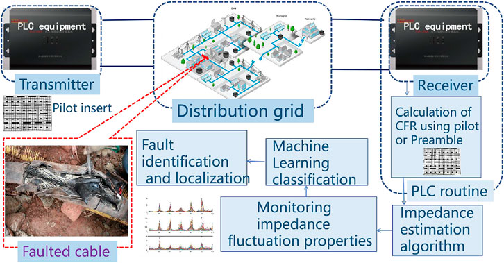
FIGURE 1. Overall scheme diagram.

Power line channel modeling

This section uses a bottom-up approach to model the PLC channel to obtain the CFR of the system (Niu et al., 2021), where CFR is the voltage ratio between two nodes (transmitter and receiver). According to the transmission line theory, the characteristics of the transmission line are mainly expressed by the characteristic impedance and transmission constant, $\mathit{Z}$; $\mathit{\gamma }$ can be obtained from equations (1); (2), which are calculated according to the resistance, inductance, conductivity and capacitance (R, L, G and C) per unit length (Meng et al., 2004; Papaleonidopoulos et al., 2003; Paul et al., 1994).

${\mathit{Z}}_{\mathbf{0}}=\sqrt{\frac{\mathit{R}+\mathit{j}\mathbf{2}\mathit{\pi }\mathit{f}\mathit{L}}{\mathit{G}+\mathit{j}\mathbf{2}\mathit{\pi }\mathit{f}\mathit{C}}}(1)$

$\mathit{\gamma }=\mathit{\alpha }+\mathit{j}\mathit{\beta }=\sqrt{\left(\mathit{R}+\mathit{j}\mathbf{2}\mathit{\pi }\mathit{f}\mathit{L}\right)\left(\mathit{G}+\mathit{j}\mathbf{2}\mathit{\pi }\mathit{f}\mathit{C}\right)}(2)$

The bottom-up channel modeling method needs to consider the network topology and simplify the network topology; As shown in Figure 2, the path between two nodes (Tx and Rx) in a typical network topology is called the trunk path (Tonello et al., 2009; Versolatto et al., 2010). All nodes on the trunk path are divided into n basic units according to the trunk path, and each basic unit has a unique trunk part and branch part; Further, the branch portion may have no branches, branches, or multiple branches. To simplify the calculation, the equivalent branch impedance of nodes with different branch levels is transmitted back to the trunk part (Paul et al., 2008). According to the bottom-up approach, each unit is divided into three parts, namely the first part, the second part and the branch part. Calculate the CFR of each basic unit. The detailed topology of each basic unit is shown in Figure 2.

FIGURE 2

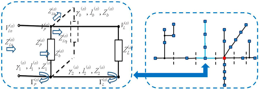
FIGURE 2. Typical network topology diagram.

As illustrated in Figure 2, the input impedance of the first part of the receiver can be obtained from the following equation:

${{{{\mathit{Z}}_{\mathit{i}\mathit{n}}}^{\left(\mathit{n}\right)}=\mathit{Z}}_{\mathbf{1}}}^{\left(\mathit{n}\right)}\hspace{0.17em}\frac{{{\mathit{Z}}_{\mathit{p}}}^{\left(\mathit{n}\right)}+{{\mathit{Z}}_{\mathbf{1}}}^{\left(\mathit{n}\right)}\mathit{tanh}\left({{\mathit{\gamma }}_{\mathbf{1}}}^{\left(\mathit{n}\right)}{{\mathit{l}}_{\mathbf{1}}}^{\left(\mathit{n}\right)}\right)}{{{\mathit{Z}}_{\mathbf{1}}}^{\left(\mathit{n}\right)}+{{\mathit{Z}}_{\mathit{p}}}^{\left(\mathit{n}\right)}\mathit{tanh}\left({{\mathit{\gamma }}_{\mathbf{1}}}^{\left(\mathit{n}\right)}{{\mathit{l}}_{\mathbf{1}}}^{\left(\mathit{n}\right)}\right)}(3)$

where ${\mathit{Z}}_1$ is the characteristic impedance, γ is the transmission constant, $\mathit{l}$ is the line length, and ${\mathit{Z}}_{\mathit{p}}$ can be obtained from the following equation:

${{\mathit{Z}}_{\mathit{P}}}^{\left(\mathit{n}\right)}=\frac{{{\mathit{Z}}_{\mathit{L}}}^{\left(\mathit{n}\right)}{{\mathit{Z}}_{\mathit{i}\mathit{n}\mathit{b}}}^{\left(\mathit{n}\right)}}{{{\mathit{Z}}_{\mathit{L}}}^{\left(\mathit{n}\right)}+{{\mathit{Z}}_{\mathit{i}\mathit{n}\mathit{b}}}^{\left(\mathit{n}\right)}}(4)$

Here, ${\mathit{Z}}_{\mathit{L}}$ is the impedance on the load side of the network, and ${\mathit{Z}}_{\mathit{i}\mathit{n}\mathit{b}}$ is the impedance on the branch side of the network. The CFR of the nth basic unit can be obtained by the voltage ratio of the receiving side to the transmitting side, expressed by the following equation:

${\mathit{H}}^{\left(\mathit{n}\right)}\left(\mathit{f}\right)=\frac{{{\mathit{V}}_{\mathit{l}}}^{\left(\mathit{n}\right)}}{{{\mathit{V}}_{\mathit{i}\mathit{n}}}^{\left(\mathit{n}\right)}}=\frac{{{\mathit{V}}_{\mathit{l}}}^{\left(\mathit{n}\right)}}{{{\mathit{V}}_{\mathit{p}}}^{\left(\mathit{n}\right)}}\frac{{{\mathit{V}}_{\mathit{p}}}^{\left(\mathit{n}\right)}}{{{\mathit{V}}_{\mathit{i}\mathit{n}}}^{\left(\mathit{n}\right)}}(5)$

$\frac{{{\mathit{V}}_{\mathit{l}}}^{\left(\mathit{n}\right)}}{{{\mathit{V}}_{\mathit{p}}}^{\left(\mathit{n}\right)}}=\frac{\mathbf{1}+{{\mathit{\Gamma }}_{\mathit{L}}}^{\left(\mathit{n}\right)}}{{\mathit{e}}^{{{\mathit{\gamma }}_{\mathbf{2}}}^{\left(\mathit{n}\right)}{{\mathit{l}}_{\mathbf{2}}}^{\left(\mathit{n}\right)}}+{{\mathit{\Gamma }}_{\mathit{L}}}^{\left(\mathit{n}\right)}{\mathit{e}}^{-{{\mathit{\gamma }}_{\mathbf{2}}}^{\left(\mathit{n}\right)}{{\mathit{l}}_{\mathbf{2}}}^{\left(\mathit{n}\right)}}}(6)$

$\frac{{{\mathit{V}}_{\mathit{p}}}^{\left(\mathit{n}\right)}}{{{\mathit{V}}_{\mathit{i}\mathit{n}}}^{\left(\mathit{n}\right)}}=\frac{\mathbf{1}+{{\mathit{\Gamma }}_{\mathit{p}}}^{\left(\mathit{n}\right)}}{{\mathit{e}}^{{{\mathit{\gamma }}_{\mathbf{1}}}^{\left(\mathit{n}\right)}{{\mathit{l}}_{\mathbf{1}}}^{\left(\mathit{n}\right)}}+{{\mathit{\Gamma }}_{\mathit{p}}}^{\left(\mathit{n}\right)}{\mathit{e}}^{-{{\mathit{\gamma }}_{\mathbf{1}}}^{\left(\mathit{n}\right)}{{\mathit{l}}_{\mathbf{1}}}^{\left(\mathit{n}\right)}}}(7)$

${{\mathit{\Gamma }}_{\mathit{L}}}^{\left(\mathit{n}\right)}=\frac{{{\mathit{Z}}_{\mathit{L}}}^{\left(\mathit{n}\right)}-{{\mathit{Z}}_{\mathbf{2}}}^{\left(\mathit{n}\right)}}{{{\mathit{Z}}_{\mathit{L}}}^{\left(\mathit{n}\right)}+{{\mathit{Z}}_{\mathbf{2}}}^{\left(\mathit{n}\right)}}(8)$

${{\mathit{\Gamma }}_{\mathit{P}}}^{\left(\mathit{n}\right)}=\frac{{{\mathit{Z}}_{\mathit{P}}}^{\left(\mathit{n}\right)}-{{\mathit{Z}}_{\mathbf{1}}}^{\left(\mathit{n}\right)}}{{{\mathit{Z}}_{\mathit{p}}}^{\left(\mathit{n}\right)}+{{\mathit{Z}}_{\mathbf{1}}}^{\left(\mathit{n}\right)}}(9)$

Where ${\mathit{Z}}_2$ is the characteristic impedance of the line of the basic unit part 2, ${\gamma }_2$ is the transmission constant of the line of the basic unit part 2, ${\mathit{l}}_2$ is the line length of the line of the basic unit part 2, ${\mathit{\Gamma }}_{\mathit{P}}$ is the reflection coefficient of the basic unit part 1, ${\Gamma }_{\mathit{L}}$ is the reflection coefficient of the basic unit part 2.

Using these equation, we can obtain the CFR of the nth basic unit. Therefore, iterating from the back to front, the CFR of each basic unit can be determined. The total channel frequency response can be obtained using the following equation:

$\mathit{H}\left(\mathit{f}\right)={\displaystyle \prod }_{\mathit{n}=\mathbf{1}}^{\mathit{N}}{\mathit{H}}^{\left(\mathit{n}\right)}\left(\mathit{f}\right)(10)$

Similarly, the CFR between any two points can be determined by simply cascading the CFR of all the essential cells between the two points.

Faulty cable model

First, when a ground fault is generated, it will cause a transient change in the topology, and this change will cause a more drastic change in the CFR and impedance spectrum.

Since the ground fault is mainly manifested in one fault point, the fault is simulated by the resistance ${\mathit{R}}_{\mathit{f}}$, the cable in case of fault is equated into a distributed parameter model, as displayed in Figure 3, to describe the transmission characteristics of the signal in the cable (Xie et al., 2017). The CFR in case of a cable fault is obtained through previously proposed channel modeling.

FIGURE 3

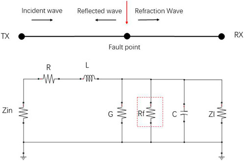
FIGURE 3. Fault cable equivalence diagram.

The resistance R, inductance L, capacitance C, and conductance G at each unit length of the cable can be approximated by the following equation (van der Wielen et al., 2008):

$\mathit{R}\approx \frac{\mathbf{1}}{\mathbf{2}\mathit{\pi }}\sqrt{\frac{{\mathit{\mu }}_{\mathbf{0}}\mathit{\omega }}{\mathbf{2}}}\left(\frac{\mathbf{1}}{{\mathit{r}}_{\mathit{c}}}\sqrt{{\mathit{\rho }}_{\mathit{c}}}+\frac{\mathbf{1}}{{\mathit{r}}_{\mathit{s}}}\sqrt{{\mathit{\rho }}_{\mathit{s}}}\right)(11)$

$\mathit{L}\approx \frac{{\mathit{\mu }}_{\mathbf{0}}}{\mathbf{2}\mathit{\pi }}\mathit{ln}\frac{{\mathit{r}}_{\mathit{s}}}{{\mathit{r}}_{\mathit{c}}}+\frac{\mathbf{1}}{\mathbf{4}\mathit{\pi }}\sqrt{\frac{{\mathbf{2}\mathit{\mu }}_{\mathbf{0}}}{\mathit{\omega }}}\left(\frac{\mathbf{1}}{{\mathit{r}}_{\mathit{c}}}\sqrt{{\mathit{\rho }}_{\mathit{c}}}+\frac{\mathbf{1}}{{\mathit{r}}_{\mathit{s}}}\sqrt{{\mathit{\rho }}_{\mathit{s}}}\right)(12)$

$\mathit{C}=\frac{\mathbf{2}\mathit{\pi }\mathit{\epsilon }}{\mathit{ln}\left({\mathit{r}}_{\mathit{s}}/{\mathit{r}}_{\mathit{c}}\right)}(13)$

$\mathit{G}=\frac{\mathbf{2}\mathit{\pi }\mathit{\delta }}{\mathit{ln}\left({\mathit{r}}_{\mathit{s}}/{\mathit{r}}_{\mathit{c}}\right)}(14)$

where the angular frequency ω = 2πf, ${\mathit{r}}_{\mathit{c}}$, and ${\mathit{r}}_{\mathit{s}}$ are the cable core version diameter and shield inner radius, respectively, ${\rho }_{\mathit{c}}$ and ${\rho }_{\mathit{s}}$ are the cable core resistivity and shield resistivity, respectively, ${\mu }_0$ is the vacuum permeability, ε is the dielectric constant of the dielectric, and δ is the dielectric conductivity. Knowing the distribution parameters of the cable, the channel can be modeled by the bottom-up presented approach above for the normal and fault cases. Its transmission characteristics change when a fault occurs, as displayed in Figure 3. When the value of ${\mathit{R}}_{\mathit{f}}$ is greater than 10 ${\mathit{Z}}_0$, it is a high impedance fault, for ${\mathit{R}}_{\mathit{f}}$ less than 10 ${\mathit{Z}}_0$, it is a low impedance fault, and ${\mathit{Z}}_0$ is the characteristic impedance of the cable (Lu et al., 2004). The high and low resistance fault sizes in this paper’s simulation section are set to 10 ${\mathit{Z}}_0$ and ${\mathit{Z}}_0$, or 500 and 50 Ω, respectively.

Fault detection theory

Eq. 3 indicates that when a ground fault occurs, the branch and backbone structure of the network changes. Changes in structure will affect the topology and reflection coefficient of the network; changes in structure will also affect the impedance of each part. Under the influence of both, the input impedance will also change (Passerini et al., 2017). Therefore, whether a fault occurs from the perspective of input impedance can be determined, and the following equation is defined from the perspective of fault detection.

$\mathit{\Delta }\left(\mathit{I}\mathit{N}\right)=\frac{{\mathit{Z}}_{\mathit{N}\mathit{F}}-{\mathit{Z}}_{\mathit{f}\mathit{a}\mathit{u}\mathit{l}\mathit{t}}}{{\mathit{Z}}_{\mathit{N}\mathit{F}}}\times \mathbf{100}\left(\%\right)(15)$

Here, ${\mathit{Z}}_{\mathit{N}\mathit{F}}$ is the input impedance under normal conditions, and ${\mathit{Z}}_{\mathit{f}\mathit{a}\mathit{u}\mathit{l}\mathit{t}}$ is under fault conditions.

However, no direct correlation was observed between CFR and input impedance in the aforementioned derivation, even though a certain mathematical relationship exists. In (Papaleonidopoulos et al., 2003), the input impedance was postulated to depend on the ratio between two functions (current transfer function and voltage transfer function) (Piante et al., 2019) as follows:

${\mathit{H}}_{\mathit{V}}=\frac{{\mathit{Z}}_{\mathit{l}}}{{\mathit{Z}}_{\mathit{i}\mathit{n}}}{\mathit{H}}_{\mathit{I}}={\mathit{Z}}_{\mathit{l}}{\mathit{Y}}_{\mathit{i}\mathit{n}}{\mathit{H}}_{\mathit{I}}(16)$

Therefore, a relationship exists between the voltage transfer function and the input impedance, and the correlation is apparent when the current transfer function is constant as follows (Piante et al., 2019):

$\frac{{\mathit{H}}_{\mathit{N}\mathit{F}}-{\mathit{H}}_{\mathit{f}\mathit{a}\mathit{u}\mathit{l}\mathit{t}}}{{\mathit{H}}_{\mathit{N}\mathit{F}}}=\frac{{\mathit{Z}}_{\mathit{l}}{\mathit{Y}}_{\mathit{i}\mathit{n}}{\mathit{H}}_{\mathit{I}}-{\mathit{Z}}_{\mathit{l}}{\mathit{Y}}_{\mathit{inf}}{\mathit{H}}_{\mathit{I}\mathit{f}}}{{\mathit{Z}}_{\mathit{l}}{\mathit{Y}}_{\mathit{i}\mathit{n}}{\mathit{H}}_{\mathit{I}}}=\frac{{\mathit{Y}}_{\mathit{i}\mathit{n}}-{\mathit{Y}}_{\mathit{inf}}\frac{{\mathit{H}}_{\mathit{I}\mathit{f}}}{{\mathit{H}}_{\mathit{I}}}}{{\mathit{Y}}_{\mathit{i}\mathit{n}}}(17)$

where ${\mathit{H}}_{\mathit{N}\mathit{F}}$ is the voltage transfer function under normal conditions, ${\mathit{H}}_{\mathit{f}\mathit{a}\mathit{u}\mathit{l}\mathit{t}}$ is the voltage transfer function under fault conditions. Furthermore, ${\mathit{H}}_{\mathit{I}}$ is the current transfer function under normal conditions, ${\mathit{H}}_{\mathit{I}\mathit{f}}$ is the current transfer function under fault conditions, and the change of input impedance before and after a fault is apparent,Y_in is the admittance value of the first part of the receiver. The fault can be monitored using the input impedance; as expressed in Eq. 17, the voltage transfer function can be used to observe the fault, and the frequency domain of the voltage transfer function is the CFR. Therefore, the fault can be detected from the perspective of the CFR, which can be measured by the PLC equipment.

Therefore, the input impedance and CFR allow the detection of faults, as shown below:

$\mathit{\Delta }\left(\mathit{I}\mathit{N}\right)=\frac{{|\mathit{Z}}_{\mathit{N}\mathit{F}}|-{|\mathit{Z}}_{\mathit{f}\mathit{a}\mathit{u}\mathit{l}\mathit{t}}|}{\left|{\mathit{Z}}_{\mathit{N}\mathit{F}}\right|}\times \mathbf{100}\left(\%\right)(18)$

$\mathit{\Delta }\left(\mathit{C}\mathit{F}\mathit{R}\right)=\frac{{|\mathit{H}}_{\mathit{N}\mathit{F}}\left(\mathit{f}\right)\left|-{|\mathit{H}}_{\mathit{f}\mathit{a}\mathit{u}\mathit{l}\mathit{t}}\left(\mathit{f}\right)\right|}{\left|{\mathit{H}}_{\mathit{N}\mathit{F}}\left(\mathit{f}\right)\right|}\times \mathbf{100}\left(\%\right)(19)$

Fault location theory

After fault detection, fault location should be determined. When the network topology changes due to faults, enough fault information can be obtained from Eqs 18, 19, which can be used to determine the fault location. Since CFR is greatly affected, the fault can be determined from the perspective of input impedance. Moreover, the input impedance is obtained by using the impedance estimation technique, which does not require additional measurement equipment and is presented in Chapter three. After obtaining the input impedance, only the input impedance is subjected to the inverse fast Fourier transform (IFFT):

$\mathit{\Delta }\left(\mathit{I}\mathit{N}\right)\stackrel{\mathit{I}\mathit{F}\mathit{F}\mathit{T}}{\to }\mathit{\Delta }\left(\mathit{t}\right)(20)$

To achieve fault positioning, the electromagnetic wave propagation speed in the cable should be calculated at high frequency. The faster the wave propagation speed is, the highest is close to the speed of light. At high frequencies, the propagation speed of electromagnetic waves is independent of frequency and is mainly determined by the primary transmission constants L and C of the cable line, and the electromagnetic wave speed can be expressed as follows:

$\mathit{v}=\frac{\mathbf{1}}{\sqrt{\mathit{L}\mathit{C}}}(21)$

Combining the wave velocity (21) with the input impedance Eq. 20 in time domain yields a function of distance.

$\mathit{d}\left(\mathit{v}\mathit{t}\right)=\mathit{\Delta }\left(\mathit{t}\times \mathit{v}\right)(22)$

Therefore, The obtained equation is a function of distance and variation, from which information about the fault location can be obtained. The input impedance is obtained through iteration easily by using the modeling process. When a fault occurs, the input impedance at the fault point and the input impedance of the node after the fault point change. Therefore, the fault location can be determined according to this characteristic.

Technical route and impedance estimation

According to the method proposed in (Liang et al., 2019), CFR is used to predict the impedance, that is, impedance estimation technology. Obtain CFR in real time through PLC equipment. According to the relationship between CFR and impedance spectrum, the characteristics of CFR are extracted by variational modal decomposition (VMD), and the key factors affecting impedance are obtained. The impedance estimation model is obtained by using the decision tree machine learning algorithm model.

Impedance estimation

The impedance estimation technique is categorized into the following steps, as displayed in Figure 4.

FIGURE 4

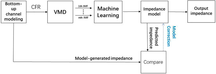
FIGURE 4. Flow chart of impedance estimation technique.

First, the CFR is obtained by modeling the channel in a bottom-up approach. A close relationship exists between the input impedance and CFR; therefore, machine learning techniques are used to predict the input impedance, using the CFR as the input and the input impedance as the output. However, some error exists when using the CFR directly as the input. Therefore, feature extraction is performed for the CFR using VMD. In this study, the impedance estimation technique was introduced using a set of CFR data as an example, and a set of channel frequency response data is displayed in Figure 5.

FIGURE 5

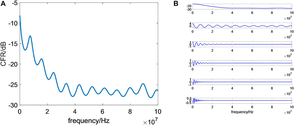
FIGURE 5. A set of CFR data and VMD result. (A) is the CFR data, (B) is the VMD result.

The CFR was then subjected to VMD decomposition and performed on the CFR data in Figure 5A to obtain six sets of eigenmode functions (IMF components), as displayed in Figure 5B. High-frequency components exist in the IMF of Figure 5B, and the high-frequency components are used as the input produces errors in the prediction results. Therefore, the IMF should be analyzed. Experimental results revealed that the first three components of the VMD decomposition were selected for superior prediction.

In the third step, machine learning is used to predict impedance. Experimental results have revealed the first three quantities in the IMF after decomposition using VMD are closely related to the impedance; therefore, after removing the curve’s high frequency noise, the first three quantities are selected as the input to the decision tree, and the amplitude and phase of the impedance are used as the output. The data from the preliminary modeling are compared to verify the accuracy of the impedance estimation technique. The results are displayed in Figure 6, which revealed that the impedance estimation technique exhibits excellent impedance prediction results; The results show that the predicted value from the simulation procedure is also in line with the set real value.

FIGURE 6

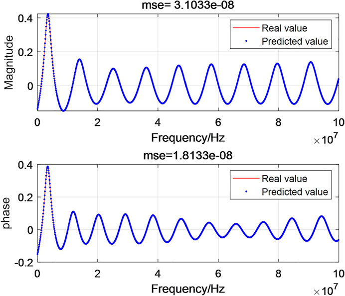
FIGURE 6. Predicted results of impedance estimation.

Impedance estimation techniques can predict impedance accurately, and the expected input impedance can be used for fault detection. When the CFR is obtained, the CFR can be used for fault detection. The impedance estimation technique can be used predict the impedance, and the input impedance can be used for fault detection and location. By contrast, the CFR can be obtained directly by using power line communication equipment.

Simulation

In this chapter, The simulation model is built in matlab software, and the transmission line model is modeled and processed by combining the bottom-up modeling method and the theory of transmission line. Combined with the change of network topology under fault conditions, the CFR of the receiving end is changed. According to the relationship between CFR and input impedance, the VMD and machine learning methods are used to predict the impedance. Then, according to the change of impedance spectrum under normal and fault conditions, the fault is monitored and the fault is located. First, a random topology using measured load data and random trunk and branch lengths is constructed, and then any set of data from it is taken for detailed analysis. Second, the fault detection is performed by CFR data and impedance data, and the fault detection effects of the two different methods are compared and analyzed, and finally, the fault location effect using the predicted input impedance is demonstrated.

The subsequent simulation will use a single-core power cable as the object of study, and simulations have been performed based on the actual parameters of the cable, and Figure 7 shows the simplified structure of the single-core cable (Wagenaars et al., 2010).

FIGURE 7

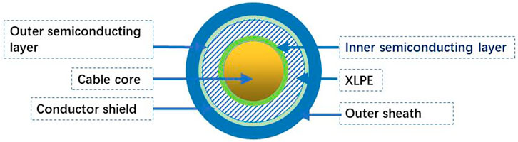
FIGURE 7. Simplified structure diagram of single-core cable.

The parameters of 240-mm² single-core cross-linked polyethylene cable (XLPE cable) are presented in Table 1, and the properties of XLPE cable are listed in Table 2.

TABLE 1

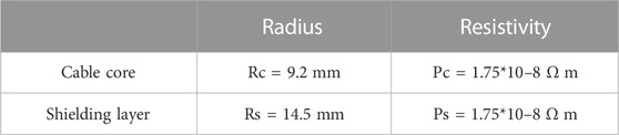
TABLE 1. The parameters of XLPE cable.

TABLE 2

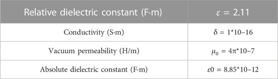
TABLE 2. The properties of XLPE.

Given the above parameters, the cable can be modeled according to the cable modeling method described previously.

First, 500 sets of CFR data under normal conditions are generated. The trunk length of each basic unit is randomly generated in the range of 1000m–2000m, the branch length is randomly generated in the range of 500m–1000m, and the load impedance is set to the measured load impedance data Xiaoxian et al. (2007). The 500 group CFR data is shown in Figure 8, each set of CFR data showed a trend of oscillation attenuation with the increase of frequency.

FIGURE 8

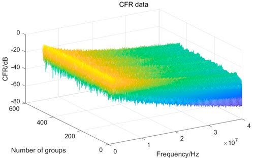
FIGURE 8. 500 sets of CFR.

Fault detection

To reflect the randomness of the extraction model, taking out any group from 500 groups of random data, and its topology is shown in Figure 9. The total length of the network backbone was 2591m, with two branches; branch lengths were 524 and 841 m respectively. The red color represents the backbone network, and it is divided into 579 m AB segment, 1172 m BC segment, and 783 m CD segment.

FIGURE 9

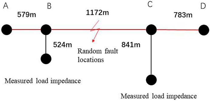
FIGURE 9. Topological network structure diagram.

First, the network displayed in Figure 9 is simulated to obtain the CFR under normal conditions, as displayed in Figure 10A.

FIGURE 10

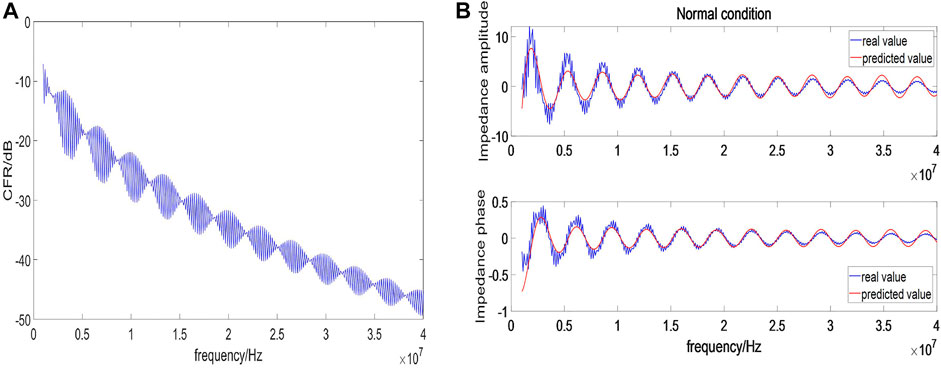
FIGURE 10. The data under normal conditions, (A) is the CFR data under normal conditions, (B) is the impedance date under normal conditions.

Based on the impedance estimation technique verified above, the system input impedance under normal conditions is predicted, and the prediction effect is shown in Figure 10B.

The input impedance changes when a grid ground fault occurs. By monitoring the input impedance at point B in Figure 9, a fault between BD can be observed because when a fault occurs in the BD segment, it causes the input impedance at point B to change. A 500-Ω high-impedance fault and a 50-Ω low-impedance fault are set in the BD segment, and the fault distance is set randomly in the BD segment; 300 sets are set in the BC segment, and 200 groups are set in the CD segment; therefore, 500 sets of fault data are generated, and 500 sets of input impedance and CFR data are shown in Figures 11A, B.

FIGURE 11

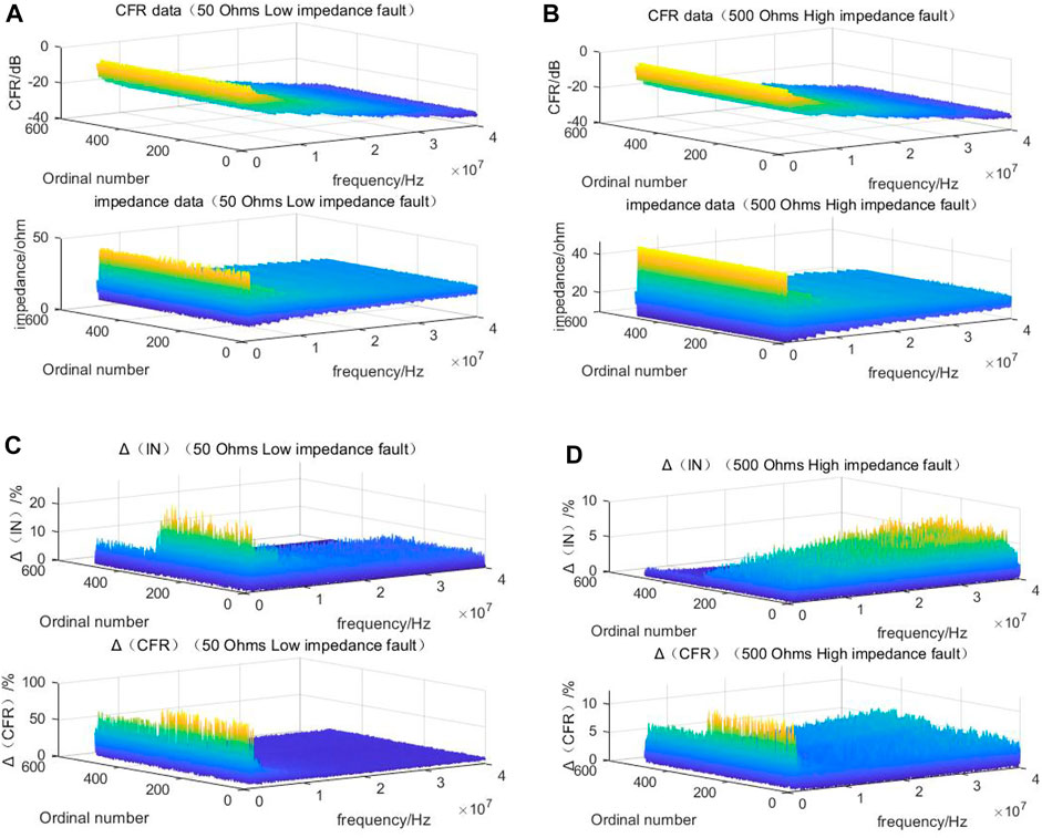
FIGURE 11. 500 sets of CFR, impedance data and Δ values. (A, B) are CFR data and impedance data for low impedance and high impedance fault, respectively(C, D) are Δ values for low impedance and high impedance fault, respectively.

Figure 11A displays a low-impedance fault with a fault impedance of 50 Ω, and Figure 11B displays a high-impedance fault with a fault impedance of 500 Ω. The 500 sets of CFR data and 500 sets of input impedance amplitude data used in the study are shown. When the CFR data and the input impedance data are obtained, the data are calculated by using Eqs 18, 19 above to obtain the Δ value characterizing the system variation obtained from the CFR and input impedance, respectively. The Δ-values for the low-impedance fault and high-impedance fault cases are displayed in Figures 11C, D.

Figure 11C details a low impedance fault with a fault impedance of 50 Ω, and Figure 11D indicates a high-impedance fault with a fault impedance of 500 Ω. Five hundred sets of Δ(CFR) and Δ(IN), obtained from CFR and input impedance, respectively.

When the Δ value is obtained, Δ(CFR) and Δ(IN) are analyzed separately. If the peak value of Δ is more significant, the system exhibits more apparent changes and can be easily monitored. The peak values of 500 sets of Δ data are illustrated in Figure 12. Eventually, the Δ data can be analyzed to obtain fault information.

FIGURE 12

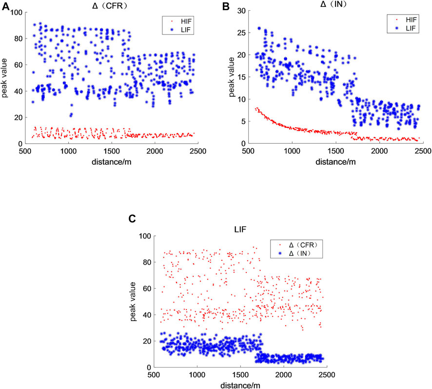
FIGURE 12. Comparison of 500 sets of Δ data. (A) is the Δ data comparison of CFR in the case of HIF and LIF. (B) is the Δ data comparison of IN in the case of HIF and LIF. (C) is the comparison of CFR and IN under LIF.

Figure 12A shows the data for Δ(CFR), Figure 12B shows the data for Δ(IN), and Figure 12C displays a comparison between Δ(CFR) and Δ(IN) for the low-impedance case. A comparison of the effectiveness of two of these techniques for monitoring faults is shown in Table 3 Figures 12A, B reveal that both different technologies have good monitoring results for high and low resistance faults, the peak value of low impedance faults is always higher than that of high impedance faults, so low impedance faults are easier to monitor. This method can be applied to monitor LIFs and HIFs. As displayed in Figure 12C, a branch exists at 1751 m in the topology. When using the input impedance for fault detection, a clear stratification is observed in Δ(IN), and also can roughly identify the fault before or after the branch; however, this effect is not clear when using CFR. And the Δ(CFR) is more significant than Δ(IN) when using CFR for fault detection. As illustrated in Figures 12C, D and Figure 12, 500 groups of random faults Δ Values have specific peaks; therefore, Δ Value can be used to detect faults.

TABLE 3

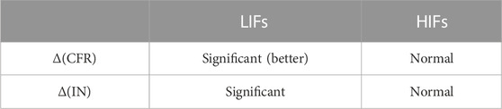
TABLE 3. Comparison of the effectiveness of different technologies for monitoring faults.

Fault location

When using the aforementioned location method for fault location, the input impedance changes when the network changes; which provides sufficient information about fault location. The topological network displayed in Figure 9 was used for fault location. Figure 13 shows the input impedance data (with actual as well as predicted values) for faults occurring at 1,000 and 1,500 m with 50 and 500 Ω. The input impedance predicted using impedance estimation techniques is then used for fault location.

FIGURE 13

FIGURE 13. Input impedance values of different faults at different locations.

When fault location is performed, the PLC device acquires the real-time CFR and estimates the current input impedance waveform from the real-time CFR. Then the IFFT of the impedance is obtained from Eq. 20. The wave speed can be obtained from Eq. 21. From the wave speed, a function (22) of distance can be obtained, by which the fault point can be located. Figure 14 shows the localization results for different fault impedances.

FIGURE 14

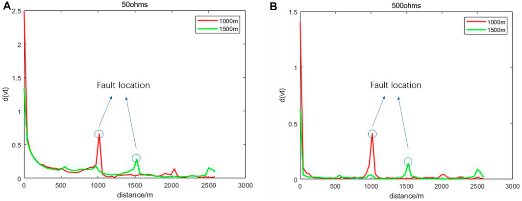
FIGURE 14. Positioning effect under different conditions. (A) is the fault location effect under LIF. (B) is the fault location effect under HIF.

The figure shows that there is a clear wave peak at the location of the 1,000 and 1,500 m point, the peak contains the location information of the fault point, the position corresponding to the peak is the position of the fault point, so the fault can be located by peak finding. Among them, the results of fault impedance localization are shown in Table 4.

TABLE 4

TABLE 4. Localization results of different fault impedances at different distances.

As presented in the table, the positioning, although a specific error exists, from the perspective of using the input impedance to locate the fault, the fault can be an approximate location of the calculation. This fault monitoring and location algorithm has a positive effect on high and low resistance fault monitoring and can be applied in fault monitoring.

If the fault occurs on the branch, the above method can also be used to detect and locate the fault. First, the receiver is connected to the branch end, the position of the transmitter remains unchanged, and the original network topology is changed. The original branch part can be regarded as the backbone part of the new topology. Then, the same method as above is used to achieve Fault detection and location.

Conclusion

An enhanced fault monitoring method based on power line carrier communication was proposed. In this method, an impedance estimation algorithm was used to monitor real-time impedance fluctuations to accomplish accurate fault location. The following conclusions were verified through theory and simulation.

1) The fault can be monitored in real time using the impedance estimation information only by computing and comparing the Δ value, and impedance positioning can be carried out in real time and with high precision within the access network, without the need for additional equipment, making it an ideal option for ground fault monitoring.

2) For high and low impedance faults occurring at 1,500–2,500 m, the proposed method can be used to achieve complete monitoring success with a localization error of approximately 50 m, while at fault locations closer than 1,500 m, the proposed method has better monitoring results and high localization accuracy. The method is not affected by fault current.

3)Although the peak value of CFR technology in monitoring high and low impedance faults is higher than that of input impedance technology, the technology proposed in this paper can not only realize the correct monitoring of high and low resistance faults, but also achieve better positioning effect. The positioning error is less than 2.13%, and online monitoring and positioning can be realized only by relying on the carrier equipment on the existing power grid.

Data availability statement

The original contributions presented in the study are included in the article/supplementary material, further inquiries can be directed to the corresponding author.

Author contributions

DL put forward the research direction, organized the research activities, provided theory guidance, and completed the revision of the article. KZ completed the principal analysis and the method design, performed the simulation, and drafted the article. All five were involved in revising the paper. All authors have read and agreed to the published version of the manuscript.

Funding

This research was supported by the National Natural Science Foundation of China (Grant No. 51707154) and the Provincial Education Department (Program No. 15JK1511).

Conflict of interest

The authors declare that the research was conducted in the absence of any commercial or financial relationships that could be construed as a potential conflict of interest.

Publisher’s note

All claims expressed in this article are solely those of the authors and do not necessarily represent those of their affiliated organizations, or those of the publisher, the editors and the reviewers. Any product that may be evaluated in this article, or claim that may be made by its manufacturer, is not guaranteed or endorsed by the publisher.

References

Aucoin, B. M., and Russell, B. D. (1982). Distribution high impedance Fault Detection utilizing high frequency current components. IEEE Power Eng. Rev. 2 (6), 46–47. doi:10.1109/MPER.1982.5521003

CrossRef Full Text | Google Scholar

Balser, S. J., Clements, K. A., and Lawrence, D. J. (1986). A microprocessor-based technique for detection of high impedance faults. IEEE Trans. Power Deliv. 1 (3), 252–258. doi:10.1109/TPWRD.1986.4308000

CrossRef Full Text | Google Scholar

Bhandia, R., Chavez, J. d. J., Cvetković, M., and Palensky, P. (2020). High impedance Fault Detection using advanced distortion detection technique. IEEE Trans. Power Deliv. 35 (6), 2598–2611. doi:10.1109/TPWRD.2020.2973829

CrossRef Full Text | Google Scholar

Cao, A., Zeman, T., and Hrad, J. (2016). “Medium-voltage faults location and handling with the help of powerline communication systems,” in 2016 17th International Conference on Mechatronics - Mechatronika (ME), Prague, Czechia, 1–4.

Google Scholar

Chul-Hwan Kim, Hyun Kim, Ko, Young-Hun, Byun, Sung-Hyun, Aggarwal, R. K., and Johns, A. T. (2002). A novel fault-detection technique of high-impedance arcing faults in transmission lines using the wavelet transform. IEEE Trans. Power Deliv. 17 (4), 921–929. doi:10.1109/TPWRD.2002.803780

CrossRef Full Text | Google Scholar

Costa, F. B., Souza, B. A., Brito, N. S. D., Silva, J. A. C. B., and Santos, W. C. (2015). Real-time detection of transients induced by high-impedance faults based on the boundary wavelet transform. IEEE Trans. Industry Appl. 51 (6), 5312–5323, Nov. doi:10.1109/TIA.2015.2434993

CrossRef Full Text | Google Scholar

García, J. C., García, V. V., and Kagan, N. (2014). “Detection of high impedance faults in overhead multi grounded networks,” in 2014 11th IEEE/IAS International Conference on Industry Applications, Juiz de Fora, Brazil, 1–6. doi:10.1109/INDUSCON.2014.7059480

CrossRef Full Text | Google Scholar

Guillen, D., Olveres, J., Torres-García, V., and Escalante-Ramírez, B. (2022). Hermite transform based algorithm for detection and classification of high impedance faults. IEEE Access 10, 79962–79973. doi:10.1109/ACCESS.2022.3194525

CrossRef Full Text | Google Scholar

Huo, Y., Prasad, G., Lampe, L., and Leung, V. C. M. (2020). “Advanced Smart Grid Monitoring: Intelligent Cable Diagnostics using Neural Networks,” in 2020 IEEE International Symposium on Power Line Communications and its Applications (ISPLC), Malaga, Spain, 1–6. doi:10.1109/ISPLC48789.2020.9115403

CrossRef Full Text | Google Scholar

Huo, Y., Prasad, G., Atanackovic, L., Lampe, L., and Leung, V. C. M. (2018). “Grid surveillance and diagnostics using power line communications,” in 2018 IEEE International Symposium on Power Line Communications and its Applications (ISPLC), Manchester, UK, 1–6. doi:10.1109/ISPLC.2018.8360200

CrossRef Full Text | Google Scholar

Huo, Y., Prasad, G., Lampe, L., Leung, V. C. M., Vijay, R., and Prabhakar, T. (2021). “Measurement Aided Training of Machine Learning Techniques for Fault Detection Using PLC Signals,” in 2021 IEEE International Symposium on Power Line Communications and its Applications (ISPLC), Aachen, Germany, 78–83. doi:10.1109/ISPLC52837.2021.9628699

CrossRef Full Text | Google Scholar

Jia, K., Bi, T., Ren, Z., Thomas, D. W. P., and Sumner, M. (2018). High frequency impedance based fault location in distribution system with DGs. IEEE Trans. Smart Grid 9 (2), 807–816. doi:10.1109/TSG.2016.2566673

CrossRef Full Text | Google Scholar

Lai, T. M., Snider, L. A., Lo, E., and Sutanto, D. (2005). High-impedance fault detection using discrete wavelet transform and frequency range and RMS conversion. IEEE Trans. Power Deliv. 20 (1), 397–407. doi:10.1109/TPWRD.2004.837836

CrossRef Full Text | Google Scholar

Lee, R. E., and Osborn, R. H. (1985). A microcomputer based data acquisition system for high impedance fault analysis. IEEE Power Eng. ReviewPER- 5 (10), 35. doi:10.1109/MPER.1985.5528687

CrossRef Full Text | Google Scholar

Liang, D., Guo, H., and Zheng, T. (2019). Real-time impedance estimation for power line communication. IEEE Access 7, 88107–88115. doi:10.1109/ACCESS.2019.2925464

CrossRef Full Text | Google Scholar

Liang, D., Wang, Y., Guo, H., Huo, Y., and Huang, C. Intelligent sensing strategy for grid anomalies using power line communication devices. IEEE Sensors J. doi:10.1109/JSEN.2022.3166899

CrossRef Full Text | Google Scholar

Lu, Honggang, Qin, Jian, and Chen, Xiangxun (2004). Overview of power cable fault location. Power Syst. Technol. 28 (20), 58–63. (in chinese).

Google Scholar

Lu, H., Zhang, W. -H., Wang, Y., and Xiao, X. -Y. (2022). Cable Incipient Fault Identification method using power disturbance waveform feature learning. IEEE Access 10, 86078–86091. doi:10.1109/ACCESS.2022.3197200

CrossRef Full Text | Google Scholar

Meng, H., Chen, S., Guan, Y. L., Law, C. L., So, P. L., Gunawan, E., et al. (2004). Modeling of transfer Characteristics for the broadband power line communication channel. IEEE Trans. Power Deliv. 19 (3), 1057–1064. doi:10.1109/TPWRD.2004.824430

CrossRef Full Text | Google Scholar

Michalik, M., Lukowicz, M., Rebizant, W., Lee, S. -J., and Kang, S. -H. (2008). New ANN-based algorithms for detecting HIFs in multigrounded MV networks. IEEE Trans. Power Deliv. 23 (1), 58–66. doi:10.1109/TPWRD.2007.911146

CrossRef Full Text | Google Scholar

Michalik, M., Lukowicz, M., Rebizant, W., Lee, S. -J., and Kang, S. -H. (2007). Verification of the wavelet-based HIF detecting algorithm performance in solidly grounded MV networks. IEEE Trans. Power Deliv. 22 (4), 2057–2064. doi:10.1109/TPWRD.2007.905283

CrossRef Full Text | Google Scholar

Milioudis, A. N., Andreou, G. T., and Labridis, D. P. (2015). Detection and location of high impedance faults in multiconductor overhead distribution lines using power line communication devices. IEEE Trans. Smart Grid 6 (2), 894–902. doi:10.1109/TSG.2014.2365855

CrossRef Full Text | Google Scholar

Milioudis, A. N., Andreou, G. T., and Labridis, D. P. (2012a). Enhanced protection scheme for Smart grids using power line communications techniques—Part I: Detection of high impedance fault occurrence. IEEE Trans. Smart Grid 3 (4), 1621–1630. doi:10.1109/TSG.2012.2208987

CrossRef Full Text | Google Scholar

Milioudis, A. N., Andreou, G. T., and Labridis, D. P. (2012b). Enhanced protection scheme for Smart grids using power line communications techniques—Part II: Location of high impedance fault position. IEEE Trans. Smart Grid 3 (4), 1631–1640. doi:10.1109/TSG.2012.2208988

CrossRef Full Text | Google Scholar

Niu, L., Wu, G., and Xu, Z. (2021). Single-phase fault line selection in distribution network based on signal injection method. IEEE Access 9, 21567–21578. doi:10.1109/ACCESS.2021.3055236

CrossRef Full Text | Google Scholar

Papaleonidopoulos, I. C., Capsalis, C. N., Karagiannopoulos, C. G., and Theodorou, N. J. (2003). “Statistical analysis and simulation of indoor single-phase low voltage power-line communication channels on the basis of multipath propagation,” in IEEE Transactions on Consumer Electronics 49 (1), 89–99. doi:10.1109/TCE.2003.1205460

CrossRef Full Text | Google Scholar

Passerini, F., and Tonello, A. M. (2017). “Power line fault detection and localization using high frequency impedance measurement,” in 2017 IEEE International Symposium on Power Line Communications and its Applications (ISPLC), Madrid, Spain, 1–5. doi:10.1109/ISPLC.2017.7897102

CrossRef Full Text | Google Scholar

Passerini, F., and Tonello, A. M. (2019). Smart grid monitoring using power line modems: Anomaly detection and localization. IEEE Trans. Smart Grid 10 (6), 6178–6186, Nov. doi:10.1109/TSG.2019.2899264

CrossRef Full Text | Google Scholar

Paul, C. R. (2008). Analysis of multiconductor transmission lines. Hoboken, NJ, USA: John Wiley and Sons.

Google Scholar

Paul, Clayton R. (1994). Analysis of multiconductor transmission lines. Newyork, NJ, USA: John Wiley.

Google Scholar

Piante, M. D., and Tonello, A. M. (2019). “Channel and Admittance Dependence Analysis in PLC with Implications to Power Loading/Savings,” in 2019 IEEE International Symposium on Power Line Communications and its Applications (ISPLC), Prague, Czech, 1–6. doi:10.1109/ISPLC.2019.8693391

CrossRef Full Text | Google Scholar

Prasad, G., Huo, Y., Lampe, L., and Leung, V. C. M. (2019). “Machine Learning Based Physical-Layer Intrusion Detection and Location for the Smart Grid,” in 2019 IEEE International Conference on Communications, Control, and Computing Technologies for Smart Grids (SmartGridComm), Beijing, China, 1–6. doi:10.1109/SmartGridComm.2019.8909779

CrossRef Full Text | Google Scholar

Routray, P., Mishra, M., and Rout, P. K. (2015). “High Impedance Fault detection in radial distribution system using S-Transform and neural network,” in 2015 IEEE Power, Communication and Information Technology Conference (PCITC), Bhubaneswar, India, 545–551. doi:10.1109/PCITC.2015.7438225

CrossRef Full Text | Google Scholar

Sedighi, A. . -R., Haghifam, M. . -R., Malik, O. P., and Ghassemian, M. . -H. (2005). High impedance fault detection based on wavelet transform and statistical pattern recognition. IEEE Trans. Power Deliv. 20 (4), 2414–2421. doi:10.1109/TPWRD.2005.852367

CrossRef Full Text | Google Scholar

Stefanidis, P. D., Papadopoulos, T. A., Arsoniadis, C. G., Nikolaidis, V. C., and Chrysochos, A. I. (2019). “Application of Power Line Communication and Traveling Waves for High Impedance Fault Detection in Overhead Transmission Lines,” in 2019 54th International Universities Power Engineering Conference (UPEC), Bucharest, Romania, 1–6. doi:10.1109/UPEC.2019.8893519

CrossRef Full Text | Google Scholar

Teng, J. -H., Huang, W. -H., and Luan, S. -W. (2014). Automatic and fast faulted line-section location method for distribution systems based on fault indicators. IEEE Trans. Power Syst. 29 (4), 1653–1662. doi:10.1109/TPWRS.2013.2294338

CrossRef Full Text | Google Scholar

Tonello, A. M., and Zheng, T. (2009). “Bottom-up transfer function generator for broadband PLC statistical channel modeling,” in 2009 IEEE International Symposium on Power Line Communications and Its Applications, Dresden, Germany, 7–12. doi:10.1109/ISPLC.2009.4913395

CrossRef Full Text | Google Scholar

van der Wielen, P. C. J. M., and Steennis, E. F. (2008). A centralized condition monitoring system for MV power cables based on on-line partial discharge detection and location. Beijing, China: International Conference on Condition Monitoring and Diagnosis, 1166–1170. doi:10.1109/CMD.2008.4580495

CrossRef Full Text | Google Scholar

Versolatto, F., and Tonello, A. M. (2010). Analysis of the PLC channel statistics using a bottom-up random simulator. Rio de Janeiro, Brazil: ISPLC2010, 236–241. doi:10.1109/ISPLC.2010.5479902

CrossRef Full Text | Google Scholar

Wagenaars, P., Wouters, P. A. A. F., Van Der Wielen, P. C. J. M., and Steennis, E. F. (2010). Approximation of transmission line parameters of single-core and three-core XLPE cables. IEEE Trans. Dielectr. Electr. Insulation 17 (1), 106–115. doi:10.1109/TDEI.2010.5412008

CrossRef Full Text | Google Scholar

Wang, B., Geng, J., and Dong, X. (2018). High-impedance Fault Detection based on nonlinear voltage–current characteristic profile identification. IEEE Trans. Smart Grid 9 (4), 3783–3791. doi:10.1109/TSG.2016.2642988

CrossRef Full Text | Google Scholar

Xiaoxian, Y., Tao, Z., Baohui, Z., Fengchun, Y., Jiandong, D., and Minghui, S. (2007). Research of impedance characteristics for medium-voltage power networks. IEEE Trans. Power Deliv. 22 (2), 870–878. doi:10.1109/TPWRD.2006.881573

CrossRef Full Text | Google Scholar

Xie, Min, Zhou, Kai, and Zhao, Shilin (2017). A new location method of local defects in power cables based on reflection coefficient spectrum. Power Syst. Technol. 41 (09), 3083–3089. (in chinese). doi:10.13335/j.1000-3673.pst.2016.2859

CrossRef Full Text | Google Scholar