 Rini Varghese P1
 M. S. P. Subathra2*
 S. Thomas George3
 Nallapaneni Manoj Kumar4,5,6*
 Easter Selvan Suviseshamuthu7
 Sanchari Deb8*
- 1Department of Electrical and Electronics Engineering, School of Engineering and Technology, Karunya Institute of Technology and Sciences, Coimbatore, Tamil Nadu, India
- 2Department of Robotics Engineering, School of Engineering and Technology, Karunya Institute of Technology and Sciences, Coimbatore, Tamil Nadu, India
- 3Department of Biomedical Engineering, School of Engineering and Technology, Karunya Institute of Technology and Sciences, Coimbatore, Tamil Nadu, India
- 4School of Energy and Environment, City University of Hong Kong, Kowloon, Hong Kong SAR, China
- 5Department of Electrical Engineering, Graphic Era (Deemed to be University), Dehradun, Uttarakhand, India
- 6Center for Research and Innovation in Science, Technology, Engineering, Arts, and Mathematics (STEAM) Education, HICCER—Hariterde International Council of Circular Economy Research, Palakkad, Kerala, India
- 7Center for Mobility and Rehabilitation Engineering Research, Kessler Foundation, West Orange, NJ, United States
- 8School of Engineering, University of Warwick, Coventry, United Kingdom
High-impedance fault (HIF) is always a threat and the biggest challenge in the power transmission and distribution system (PTDS). For a PTDS to operate effectively, HIF diagnosis is essential. However, given the HIF’s nature and the involved complexity, detection, identification, and fault location are difficult. This will be even more complicated in conventional PTDSs as they are inefficient and highly vulnerable. Given the importance and urgent need for HIF diagnosis in PTDS, this study reviews state-of-the-art HIF phenomenon and detection techniques and proposes the use of “various signal processing techniques for fault feature extraction” and “ different classifiers for identifying HIF.” First, HIF current/voltage signals are analyzed using signal processing techniques, which include the discrete wavelet transform (DWT), pattern recognition, Kalman filtering, TT transform, mathematical morphology (MM), S transform (ST), fast Fourier transform (FFT), principal component analysis (PCA), linear discriminant analysis (LDA), and wavelet transforms, such as dual-tree, maximum overlap discrete wavelet transform (MODWT), and lifting wavelet transform (LWT). Second, the various HIF and non-HIF faults are classified using intelligent classifiers. The intelligent classifiers include artificial neural networks (ANNs), probabilistic neural networks (PNNs), genetic algorithms (GAs), fuzzy logic, adaptive neuro-fuzzy interface system, support vector machine (SVM), extreme learning machine (ELM), adaptive resonance theory, random forests (RFs), decision trees (DTs), and convolution neural networks (CNNs). In addition to the comparative discussion of various classifier techniques, their evaluation criterion and performance are prioritized. Third, this review also studied different test systems, such as radial distribution network, mesh distribution network, IEEE 4 node, IEEE 13 node feeder, IEEE 34 node feeder, IEEE 39 node feeder, IEEE 123 node feeder, Palash feeder, and test microgrid systems, to assess the pertinence of various HIF detection schemes and the behavior along with methods to locate the HIF. Overall, we believe this review would serve as a comprehensive compendium of advanced techniques for HIF diagnosis in different test systems.
1 Introduction
Faults are often observed in electrical power transmission and distribution systems (PTDSs). The faults in a PTDS will distract the current from the intended path (Ali et al., 2014; Russell and Benner, 1995). The fault causes an irregular condition that decreases the strength of insulation between the conductors (Russell and Benner, 1995; Theron et al., 2018). There are numerous fault types, among which high-impedance faults (HIFs) are critical. HIF occurs when a conductor touches a tree with a high impedance or when a broken conductor touches the ground (Chen et al., 2013; Aljohani and Habiballah, 2020a). The HIF draws non-predictable currents from the distribution network, sometimes leading to arcing (Chen et al., 2013). This is visually represented and shown in Figure 1. Such faults can impose fire risks and cause an electrical shock that endangers electrical system operators, engineers, live stocks, and individuals' lives (Aljohani and Habiballah, 2020a; Sultan et al., 1994). In industrial applications, HIF detection is inevitable to ensure the safety of working persons and equipment and continuity in the service for critical loads. Thus, HIF detection and diagnosis are vital to ensure safety and continuous PTDS operation. However, its detection is quite challenging because HIFs are often not recorded as faults; hence, the reported cases are fewer than the observed ones (Ali et al., 2014). As the fault current draws less current, it remains unnoticed and persists for days. Owing to small fault currents, HIFs are difficult to detect using traditional protection relays and should be addressed through algorithms. HIF depends on various factors, such as the ground surface type, humidity, type of conductor, environmental conditions, and voltage degree, of which surface humidity and surface materials are the most influenced (Sedighizadeh et al., 2010). Many HIFs have similar features that can be represented because of differences in the arc parameters, such as conductance and time constant (Vyshnavi and Prasad, 2018; Chen et al., 2016). Low impedance fault (LIF) (Kavaskar and Mohanty, 2019; Kannan and Rathinam, 2012) is short-circuiting, followed by a high current that is sensed by a breaker.
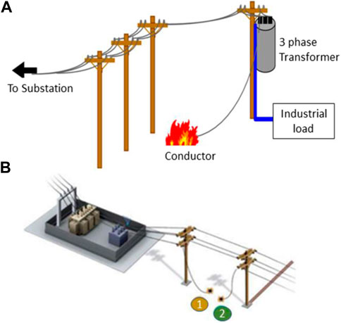
FIGURE 1. HIF in the downed conductor. (A) Arcing in the downed conductor. (B) Source end and load end conductors (Roberts et al., 2001; Suliman and Ghazal, 2019).
Arc type fault (HIF) usually occurs when a current-carrying conductor touches the ground or with another conductor through a high-impedance medium for a short time. HIF is a disturbance in a power system of approximately 15–25 kV that blocks the current required to trip the overcurrent relay (Ali et al., 2014; Calhoun et al., 1982). The voltage–current characteristics are highly dependent on various materials (Ali et al., 2014), including tree branches, lawns, gravel, stout gravel, asphalt, concrete, crushed stone, board blocks, and cement (Russell et al., 1988). Furthermore, deteriorated insulators due to cracks, dust, humidity, and ice, among others, are some of the main triggers of HIF in PTDSs (Langeroudi and Abdelaziz, 2020). The long-term persistence of HIF is undesirable for profitable and smooth operations (Langeroudi and Abdelaziz, 2020). Various faults and incorrect operations can cause blackouts (Kjølle et al., 2006). Various vulnerable surfaces to HIF with the corresponding fault currents as indicated by Sedighizadeh et al. (2010) and Tengdin et al. (1996) are wet sand 15A, dry sod 20A, dry grass 25A, wet sod 40A, wet grass 50A, reinforced concrete 75A, dry asphalt <1A, and dry sand <1A. HIFs are sub-classified into active and passive faults (Jota and Jota, 1999). Active faults possess fault currents below the threshold values of protection relays accompanied by an electric arc. An electric arc does not follow passive faults. They are challenging to detect as there is no indication of the energization of the conductor and can be detected by phase unbalance analysis. The studies evaluated that approximately 10% of the distribution faults in power systems are HIF, of which 25%–32% of the down conductors are not detected with overcurrent relays (Sultan and Swift, 1992). Hence, the detection and isolation of HIF become important. Studies show that conventional protection methods identify only 17.5% of staged HIFs, but the introduction of hybrid energies to distribution grids made the HIF detection demand necessary. An efficient detection method of HIF became necessary to eliminate false tripping and stabilize the power supply. Unlike other faults that endanger electrical appliances, HIF threatens human life. The formation of flammable gases after a HIF interception, which is near flammable material, can cause a fire or explosion. HIF can be caused by a broken or unbroken conductor. Figure 2 shows ice and a tree causing HIF in unbroken and broken conductors (Theron et al., 2018).
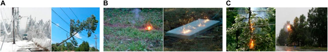
FIGURE 2. (A) Ice and a tree causing HIF in unbroken conductors (Theron et al., 2018). (B) HIF arcing on grass (Sedighizadeh et al., 2010) and concrete (Carpenter et al., 2005). (C) Unbroken conductors (Louis, 2015).
As shown by Gururajapathy et al. (2017), faults in power systems can be broadly classified into symmetrical or asymmetrical faults and balanced or unbalanced faults, among which unbalanced loads are more frequent and can be categorized as series and shunt faults. Series faults are caused by broken conductors or otherwise unbalanced series impedances. These faults can be recognized by an increase in voltage and frequency and a reduction in the current of the faulty feeder. However, in the shunt fault, there will be a fall in frequency and voltage and a rise in current, which is common in power systems. The percentage of occurrence in the power system for a single-line-to-ground fault (SLGF) is 70% which, is less severe. In line-to-line fault (LLF), it is 15%, and the severity is less. In LLF, it is 10% and less severe, whereas the triple-line-to-ground fault (LLLGF) is more severe, and occurrence is only 5%. When any phase of the transmission system comes in contact with the ground or neutral wire, an SLGF occurs due to wind and tree falling, among others. In LLF, the occurrence can be due to heavy wind or when two conductors contact each other, which can happen in overhead and underground systems. The variation of impendence spreads over a wide range in this case, and it is difficult to predict the upper and lower limits. Double-line-to-ground fault (DLGF) occurs when a tree falls on the two phases of the transmission system connecting the ground, which is considered asymmetric and a severe event if not cleared in a certain time. LLLGF is symmetrical owing to equipment failure or a tower falling on the transmission line. This is considered a serious situation as the voltages become zero, and the current may be too high. Low fault current resulting from contact with the high-impedance surface, asymmetry (Sultan et al., 1994) resulting from the presence of silica on the contact surface, randomness (Benner et al., 1989) resulting from rapid electrical discharges and floating conductors on the surface of the field, and non-linearity resulting from the different soil layer resistivity (Ali et al., 2014) are the key characteristics of the HIF. The non-linearity results from the fact that the HIF characteristic curve of the voltage–current is non-linear. Low-frequency components are present in the voltage and current waveform due to the non-linearity of HIF, which can range up to 600 Hz for current and 300 Hz for voltage. The fault current has different waveforms, and a disparity in the peak value and shape is called asymmetry for the positive and negative half periods. HIF is called an arcing fault because it is preceded by an arc, producing a few cycles of conduction followed by cycles of non-conduction. The current HIF value increases for a few cycles and holds a constant value. The current range changes over time, making it non-stationary. Random values are both the current magnitude during conduction and non-conduction periods. Arc results in the present waveform’s high-frequency components, and because of the non-linearity of the HIF waveform, it contains harmonics. HIF normally occurs at medium voltages and becomes severe at low voltages and less severe at a high voltage above 25 kV. HIF is influenced by several factors, such as feeder configuration, voltage level, weather conditions, and load type (Louis, 2015). HIF detectors find it hard to detect conductors in run-out conditions or undergo severe weather conditions, tree contacts, and a history of excessive breakage. Researchers working on HIF detection concentrated on lab-based staged fault studies. Owing to the critical nature of the faults, industry and academia focus more on simulations and software studies. Early and accurate fault detection will reduce interruption time and increase the safety and reliability of the power system. Advanced signal processing techniques depend on specialized knowledge and the accuracy of the measured data. The modern power system is currently challenged by the growing volumes of data of different natures, the need for data storage, the introduction of distributed generations, and technological advancements. However, the simulation techniques are still in their developing state. During the signal processing analysis, the hidden characteristics of the measured data are revealed, such as randomness, non-linearity, and asymmetry. Machine learning techniques can acquire hidden data from the measured data, thus providing a promising way to meet the challenges in the power system. These fault characteristics are used by the classifiers to discriminate HIFs from other disturbances.
2 HIF detection
The power system network generally has a healthy state and a faulty state. The fault identification task has three main steps: measurements (current, voltage, current and voltage, and magnetic field intensity), feature extraction, and classification (Carr, 1981). Signal processing techniques are frequently used to increase the effectiveness of HIF detection techniques. The signal processing techniques’ characteristics extracted their hidden characteristics and measured the three-phase voltage/current signals for HIF detection, improving versatility, stability, and economy. Based on these extracted features, the classifier discriminates whether the HIF event occurred.
Figure 3 shows the basic steps involved in HIF detection using signal processing techniques. The signal processing techniques commonly used for HIF detection schemes are discrete wavelet transform (DWT) (Elkalashy et al., 2007a; Elkalashy et al., 2008; Elkalashy et al., 2007b; Ibrahim et al., 2010a), principal component analysis (PCA) (Sarlak and Shahrtash, 2008), linear discriminant analysis (LDA) (Sarlak and Shahrtash, 2008), continuous wavelet transform (CWT), extended Kalman filter (EKF) (Soheili et al., 2018), time–time transform (TTT) (Nikoofekr et al., 2013), dual-tree complex wavelet transform (DTWT) (Moravej et al., 2015), S transform (ST) (Routray et al., 2016), maximum overlap discrete wavelet transform (MODWT) (Kar and Samantaray, 2017), fast Fourier transform (FFT) (Bin Sulaiman et al., 2017), Stockwell transform (Balser et al., 1982), mathematical morphology filters (MMF) (Sekar and Mohanty, 2018), and lifting wavelet transform (LWT) (Narasimhulu et al., 2020). The description of these signal processing tools used in HIF detection techniques is discussed in Section 2.3, emphasizing time-domain analysis, frequency-domain analysis, and time–frequency-domain analysis. The selected features are extracted from the input signal and then compared to a threshold value in signal processing techniques for HIF detection. Setting the threshold value is challenging because HIF would not be detected if the threshold is set too high. If it is set to an extremely low value, the relay will trip even with light disturbances. This issue can be resolved by introducing intelligent classifiers along with signal processing techniques.
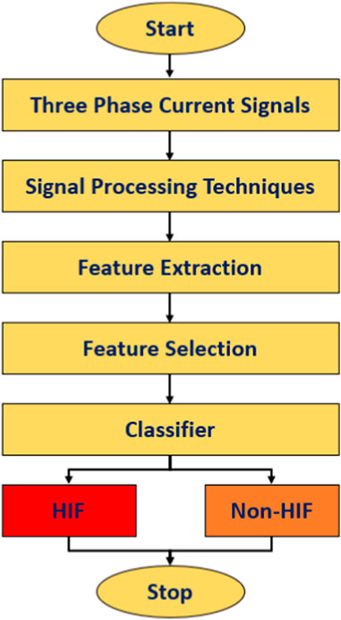
FIGURE 3. Steps involved in pattern classification of HIF detection.
Commonly used intelligent classifiers in signal processing-based HIF detection techniques are probabilistic neural network (PNN) (Samantaray et al., 2008), artificial neural network (ANN) (Baqui et al., 2011), adaptive resonant theory (ART) neural network and Fuzzy ARTMAP (Nikoofekr et al., 2013), extreme learning machines (ELMs) (Reddy et al., 2013), genetic algorithm (GA) (Xie et al., 2013a), support vector machine (SVM) (Bhongade and Golhani, 2016), adaptive neuro-fuzzy inference system (ANFIS) (Veerasamy et al., 2018), decision tree (DT) (Sekar and Mohanty, 2018), random forest (RF) (Sekar and Mohanty, 2020), convolution neural network (CNN) (Fan and Yin, 2019), and fuzzy logic control (FLC) (Suliman and Ghazal, 2019) explained in Section 4. These intelligent classifiers improved the efficiency, speed, and accuracy of signal processing-based procedures by detecting HIFs without the use of threshold settings.
The practical detection of HIFs was explained by Kistler et al. (2019), who used two relay-based HIF detection algorithms. The former uses the odd-harmonic contents of phase current, whereas the latter uses the inter-harmonic contents. The first algorithm uses total odd harmonic content from phase currents using the FIR filter. A threshold value was set, and the odd harmonic contents were compared. If the difference is more significant than the threshold, the counter increments, and the alarm is set. The second algorithm uses the sum of the difference of inter harmonic content that uses a reference and compares it to the measured sum of difference currents to detect the increase in the sum of difference currents during an HIF. The second algorithm was more successful for HIF detection, mainly on grassy surfaces, and slightly less for fully contact good insulators that do not cause an arc. The algorithm’s performance was tested in a live conductor by the Electric Power Research Institute and PPL electric utilities (SEL, 2007).
Mitigation of forest fires and human safety issues were addressed by Gashteroodkhani et al. (2021) through the practical detection of HIFs. Two strategies for fault current detection, one based on the non-harmonic content of fault currents and the other on the odd-harmonic content of fault currents, are explained and evaluated in a hardware-in-the-loop (HIL) platform employing a real-time digital simulator (RTDS). With 1,736 relay events reported, the first algorithm detected 95% of the HIFs, whereas the second detected only 5% of HIFs. The test system chosen was from a distribution network in the Northern Nevada area with a 14.4-kV three-phase three-wire feeder. Chakraborty and Das (2019) explained that smart meters are installed for voltage measurements compared with a threshold value to detect the presence of HIFs. It is tested in six different situations of three broken and three unbroken conductors. The method is implemented along with a single-phase energy meter capable of detecting the presence of HIFs, voltage sag-swells, capacitor/load switching (Panigrahi et al., 2018; Prasad et al., 2022), transformer and feeder energization (Biswal et al., 2022), power electronic loads, arc furnace loads, and distributed generators (DG). The method gives satisfactory results in HIF detection. The detection methods proposed in previous studies (Lima et al., 2018; Yang et al., 2006; Sedighi et al., 2005a; Abdelgayed et al., 2017; Wang et al., 2019) also experimented on real-time systems discussed in the various sections of the manuscript. Discrimination of HIF along with cross-country faults was explained by Ashok and Yadav (2021). A simulation model of the IEEE 13-bus system is used to obtain the three-phase current signals, and MODWPT is used for feature extraction. The real-time field data from Chhattisgarh State Power Transmission Network are collected and tested using the same algorithm. Classification of HIF, non-HIF boundary fault conditions, capacitor switching, reactor string switching, load switching, power swing effects, the effect of noise, lightly load conditions, and electric arc furnace effects in PTDSs is done. The classification is conducted by setting a threshold value for the energy envelop index. The response time of the proposed method for each case is recorded, which is less than 14.3 m. When compared with earlier studies (Ghaderi et al., 2017; Sedighizadeh et al., 2010; Vyshnavi and Prasad, 2018, this study gives an insight into various test systems used for testing various HIF detection methods and studies the nature of HIF, which is discussed in Section 3.
2.1 Measurements
Measurements such as current measurement, voltage measurement, and both current-voltage measurements extract features for fault analysis. An HIF is accompanied by the intermittence of arc (Chen et al., 2013). The arcing fault contains low- and high-frequency components in the current frequency spectrum. The low frequency-based technique results in lower-order harmonics with even, odd, and intermittent harmonics extracted for HIF detection. High frequency-based techniques show short variations in the HIF current.
Voltage measurement is performed by extracting three-phase voltage signals proposed by Ali et al. (2014) during the HIF phenomenon in an underground distribution network. Bakar et al. (2014) performed a voltage measurement at the primary substation and compared fault features with the database generated from the simulation. The method has a single measurement and multiple branches that can detect multiple faulty sections. Detection of HIFs by voltage measurement is efficient only when there is a voltage drop between the relay and fault location. The proposed method by Wang et al. (2018) used the discriminant vector of negative and zero sequence current and voltage in the substation.
Current and voltage measurement has improved reliability compared to the latter measurements. Magnetic field intensity measurement increases the cost and complexity of the detection technique (Bahador et al., 2018).
2.2 Signal processing techniques and feature extraction
Signal processing techniques are widely used to improve the effectiveness of high-impedance defect detection approaches. Signal processing techniques extract the hidden properties of observed three-phase signals for HIF detection, enhancing adaptability, stability, and cost-effectiveness. More informative data are obtained using various analyses based on these extracted data, such as time-domain analysis, frequency-domain analysis, and time–frequency analysis (Chen et al., 1990; Sarlak and Shahrtash, 2013). Table 1 gives a detailed comparison of various signal processing techniques for HIF detection using intelligent classifiers.
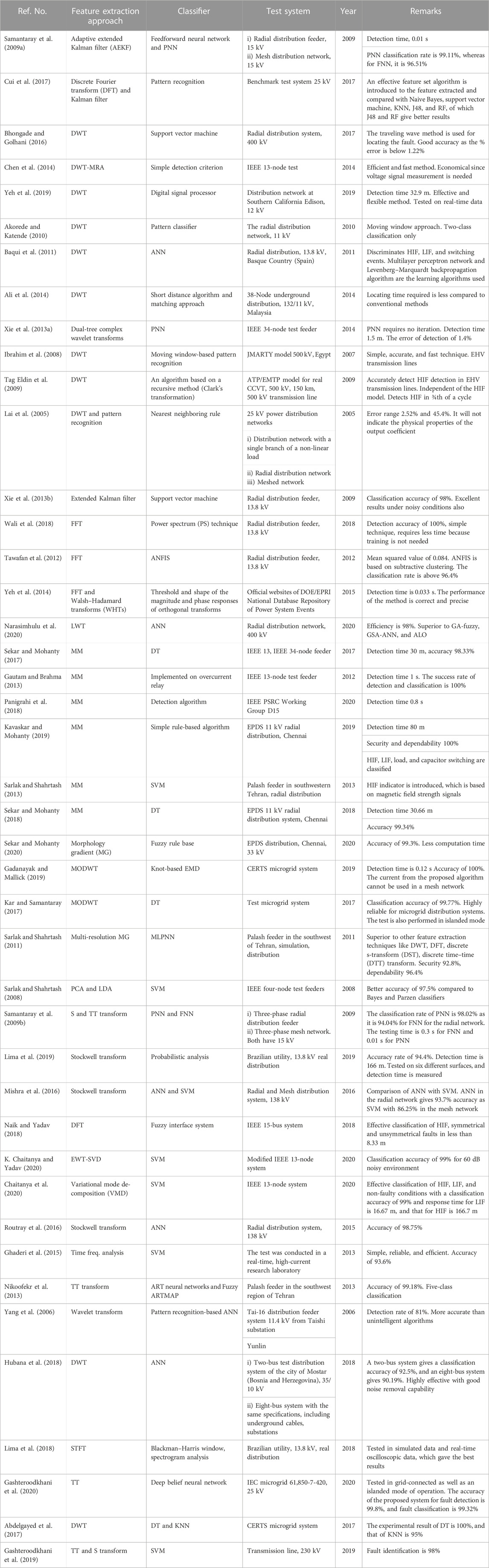
TABLE 1. Comparison of various signal processing techniques for HIF detection using intelligent classifiers.
2.3 Domain analysis
2.3.1 Time-domain analysis
The time-domain analysis uses the measure of zero-sequence voltage and current for feature extraction of HIF. The time-domain analysis is based on arc current waveform. Time-domain takes out the temporary irregularities in the HIF waveform, making the system computationally complex (Lee and Bishop, 1985).
Nezamzadeh-Ejieh and Sadeghkhani (2020) proposed that Kullback–Leibler divergence extracts the non-linearity and asymmetry characteristics of two half-cycles of the current waveform from the substation in a time-domain detection of HIF. The method is tested in 13-node and IEEE 34 systems (the Institute of Electrical and Electronics Engineers). Without any harmonic component analysis or training set, the method can identify an HIF by calculating the energization of feeders, voltage swag, and swell.
Mathematical morphology (MM) is a signal processing technique applied to issues in the power system illustrated in the literature (Sekar and Mohanty, 2018; Panigrahi et al., 2018). MM uses simple arithmetic operations, such as set theory and integral geometry, and due to its simple calculations, the processing time is less.
The basic functions in MM are dilation and erosion (Kavaskar and Mohanty, 2019). MM is non-linear, and it is time-domain processing of the signal widely used to extract high- and low-frequency signals. Here, the proposed MM, along with data mining DT, is used for HIF detection. Statistical features are extracted, which serve as input to DT and RF for discriminating with non-HIF conditions (load switching, capacitor switching, and inrush current).
The morphology gradient filter extracts statistical features from the features. A rule set is created using RF, which will accept the crisp inputs using a fuzzy-based algorithm proposed by Sekar and Mohanty (2020). This method detects HIFs and normal events with high dependability. The chosen sampling rate was 60 samples/cycle, requiring less memory space and less computational time.
The adaptive extended Kalman filter (AEKF) estimates the harmonic components in fault currents for non-linear loading conditions (Samantaray et al., 2009a). The harmonic components estimated by the technique are fundamental, third, fifth, seventh, eleventh, and thirteenth harmonics. Based on the Kalman filtering principle, Girgis et al. (1990) built an approach based on the time-varying existence of the fundamental and harmonic components to obtain the best estimate of the time variations of the harmonic components. Faridnia et al. (2012) presented a partial co-relation function for HIF detection from voltage and current relays. The method is tested in a radial feeder system with two HIF models in PSCAD/EMTDC. Twelve indices-based correlation function is implemented and tested on a wide data set to obtain accurate results for HIF detection.
2.3.2 Frequency-domain analysis
Frequency-domain analysis extracts harmonics in the current spectrum. In the current spectrum, an HIF event will produce low- and high-frequency components. Low-frequency components are based on non-linearity results, whereas high-frequency components are based on sudden and random changes in a non-stationary HIF current waveform. FFT extracts the current signal data after the simulation is applied to a power spectrum (PS) technique that can detect an HIF and distinguish it from non-faulty conditions, such as capacitor banks, non-linear loads, and linear loads, which have the same features (Wali et al., 2018). FFT is used to calculate the impulse response of the frequency domain (Scott, 1994). Aucoin and Russell (1982) utilized high-frequency current components to detect HIF. The low-frequency spectrum is compared with the harmonics of the current waveform measured in the primary substation over a week (Emanuel et al., 1990).
2.3.3 Time–frequency domain
The wavelet methods are more potent as they extract the frequency and instant or position for signal analysis. Time–frequency analysis (TFA) could effectively detect discontinuities, repeated patterns, and non-stationary aspects of signals. It measures the energy of the signal at each moment of time and frequency coordinates. TFA has been successfully applied to various power system applications, such as the evaluation of power efficiency, security of power systems, and pathfinding for disturbances of capacitor switching.
Lima et al. (2018) proposed a method that uses a short-time Fourier transform for feature extraction that extracts harmonic components of phase current as of the magnitude and phase of the third harmonic component and magnitude of second and fifth harmonics to identify the presence of HIFs. The window length chosen is directly proportional to frequency resolution and inversely proportional to time resolution. The sampling frequency is 15.6 kHz. A Brazilian distribution feeder of 13.8 kV is used to evaluate the methodology. A Blackman–Harris window with five cycles is chosen for this method, and the spectrum analysis is performed. The method was tested in sand, asphalt, gravel, grass, cobblestones, and local soil. The detection time is less than 200 ms.
The ST is an extended wavelet transform class based on Gaussian window shifting and scalable localizing. The S transform has absolute phase information and good time–frequency resolution for all frequencies. Unlike wavelet transformation, the ST is extremely resistant to noise (Mishra et al., 2016). Morlet wavelet transform differentiates between HIFs and regular switching events and investigates faults for different surfaces, including Portland cement, wet soil, and grass (Huang and Hsieh, 1999). DWT decomposes time-domain signals into different harmonics in the time–frequency domain, and the extracted features are used to train ANN (Baqui et al., 2011). The mother wavelet of Daubechies is superior to others, such as Morlet, symet, and rbior, as it can accurately detect low-amplitude signals. The method was also verified on various wet and dry surfaces.
The proposed method uses DWT, and high- and low-frequency voltage components at various system points are measured (Santos et al., 2017). The energy spectrum of the detailed and approximation coefficient is calculated. The method is evaluated using a 13.8-kV Brazilian distribution feeder with a signal-to-noise ratio (SNR) of 60 dB, and the two-time varying resistances HIF model is used. The method requires no monitoring devices and information about the feeder and load parameters. The method is reliable and efficiently identifies the HIF with a 70% search field reduction obtained.
Wavelet transform decomposes and extracts the features, PCA performs feature selection, and the Bayesian classifier discriminates the HIF with normal events (Sedighi et al., 2005a). Various tests were conducted on wet and dry surfaces. A pattern recognition system is proposed and is simulated using EMTP software. A real-time experiment is performed in Qeshm island, Iran, and an HIF is created in 8,209 m and 8,446 m locations from the site. The sampling rate of the data is 24.67 kHz, and the classifier success rate is 97.6%.
In (Li and Li, 2005) arc fault detection with automatically modified time windows to differentiate arc fault from non-arc fault is done using wavelet packet transform-based. At level 3 decomposition, db10 is used at a sampling frequency of 12.5 kHz. The window length in this study is 1/2 cycle (1.25 ms in 400 Hz for an airplane). The size of the moving window is 1/4 cycle (0.625 m in 400 Hz), such that ∆t = 0.625 m. The proposed method is powerful with simple calculations.
Michalik et al. (2006) proposed an approach in which a wavelet-based measurement is performed for zero-sequence voltage and current signals. This method gave fast and reliable HIF detection and location and obtained better performance compared to conventional methods. ANN is used for classification, and the decision module is implemented in real-time using a single neuron. The proposed method gives good results with low-impedance permanent ground faults.
Lazkano et al.’s (2004) method is based on the decomposition of three-phase unbalanced current data utilizing wavelet transform techniques. Arc phenomena linked with an HIF can be detected due to the WT’s time-frequency characteristic, and the signal is broken down into frequency sub-bands. The Db4 mother wavelet was chosen for the four-level decomposition of the arc current signal. A 20-kV Tuejar feeder of Spain is selected and simulated to test the proposed method, which gives satisfactory results.
De Alvarenga Ferreira and Mariano Lessa Assis (2019) illustrated a novel approach for HIF detection in smart grids using multi-resolution signal decomposition to decompose the DWT coefficient. The HIF model used for testing is the Kizilcay arc model. The IEEE 13-node test feeder simulated in PSCAD/EMTP is used to evaluate the proposed method. Level 3 decomposition with db8 mother wavelet function is adopted for the proposed work. Various conditions are illustrated with HIF and non-HIF conditions, such as capacitor switching. The method provides robust, fast, and reliable HIF detection.
Features of Earth faults due to leaning trees are extracted from the phase currents and voltages using the DWT (Elkalashy et al., 2007b; Elkalashy et al., 2007a; Elkalashy, 2007). The detailed coefficient of current and voltage is used, whose product is taken to compute power. A positive polarity of power gives a healthy feeder, and negative polarity gives a faulty feeder. The method has been tested on a leaning tree in a laboratory setup.
The wavelet-based algorithm is used to detect HIF detection (Michalik et al., 2007). The algorithm works great for ground fault currents above 3A, irrespective of phase and location. The method is tested in the Next-Generation Power Technology Center and KEPCo, South Korea. The sampling rate is 10k Hz, and the detection time ranges from 0.2 to 0.7s depending on the distance.
Stockwell’s transform extracts the parameters in both the time and frequency domains proposed by Lima et al. (2019) that select the statistical features discussed in Table 1. The simulated data and real-time field data (from the substation) provide the two databases for the method validation that can discriminate an HIF with other power system disturbances. The method is efficient and accurate in action.
Balser et al. (1982) utilized Hilbert transform (HT) for HIF detection in transmission lines in which an uncompensated line, series compensated line, single-pole tripping situation, and a load change are tested. The method is simulated in MATLAB/SIMULINK, and the data sampling rate is 1 kHz. An HIF detector is placed in certain locations that indicate whether a fault occurred. The method gives good accuracy and consistency. The HIF detection method using optimal transient extracting transform (OTET) was proposed by Prasad et al. (2022) and can be used in grid-connected and islanded mode systems, and is also reliable in unbalanced and harmonic contaminated signals. Biswal et al. (2022) reconstructed the features extracted from the current signals using the Savitzky–Golay filter (SGF) using the matrix pencil method (MPM), and the Teager energy of the error is estimated. The proposed method is verified in the Aalborg test feeder and modified IEEE 30-bus test systems and proven with an accuracy of 98.6%.
3 Test systems
In this section, various test systems are discussed for HIF detection. The various standard test systems were selected and simulated using MATLAB/SIMULINK, PSCAD, EMTP-RV, EMTP-ATP, and a real-time laboratory setup to investigate the performance of the different algorithms for HIF location and detection. Faults at the distribution system are a priority because the risk is greater relative to HIFs at the transmission level. An acceptable test system is selected for a suitable case study for simulation purposes and performance validation of the proposed methods. Proper data signals from the power system must be obtained under various possible operating scenarios to validate the proposed approaches. For technological and economic reasons, field fault testing on actual power systems is known to be difficult, with field test findings often having certain limitations. PDS must be correctly modeled because of these reasons. Table 1 gives a detailed discussion of various signal processing techniques for HIF detection using intelligent classifiers with various test systems used. Table 2 gives a comparison of various test systems used in HIF detection.
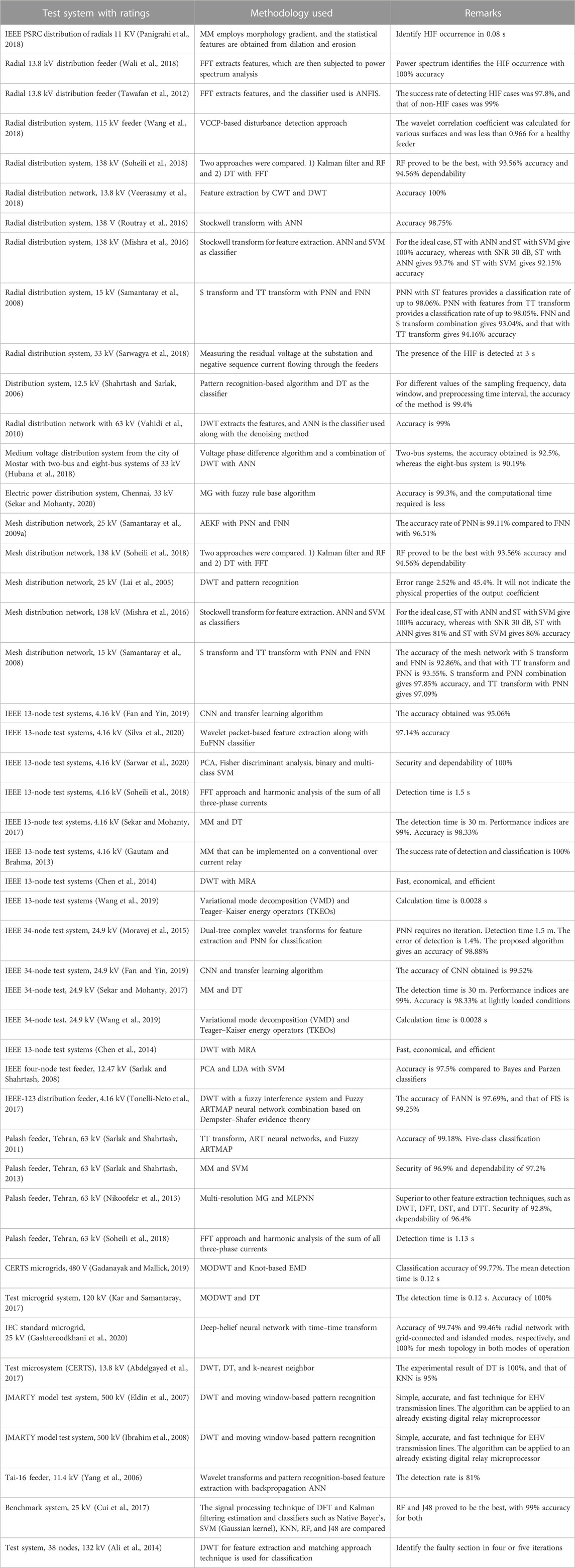
TABLE 2. Comparison of various test systems.
3.1 Radial distribution network
Shahrtash and Sarlak (2006) used a pattern recognition-based approach for HIF detection with DT as the classifier. The power distribution system is illustrated in which the system voltage is 12.5 kV, the short circuit level (at the infinite bus) is 866 MVA, and a time constant of 45 ms is shown in Figure 4A. The following data about transmission lines are given inductance of transmission line of 825 nH/m, resistance of transmission of 313 Ω/m, and line length of 33 km. The loads connected are a capacitor load rated 4.08 MVAr, transformer (10/0.4 kV) connected in delta-star, three-phase thyristor converter as harmonic load, and nominal load current of 630 A. The best results are obtained in even, odd, and in-between harmonics below 400 Hz. The classification factor is based on entropy, which is the effectiveness of an attribute in classifying data. A total of 2,583 and 1,331 cases were used for training and testing purposes, respectively. For different values of the sampling frequency of 2 kHz, a data window size of 2 cycles, and a pre-processing-time interval of 30 cycles, the accuracy of the proposed method was 99.4%.
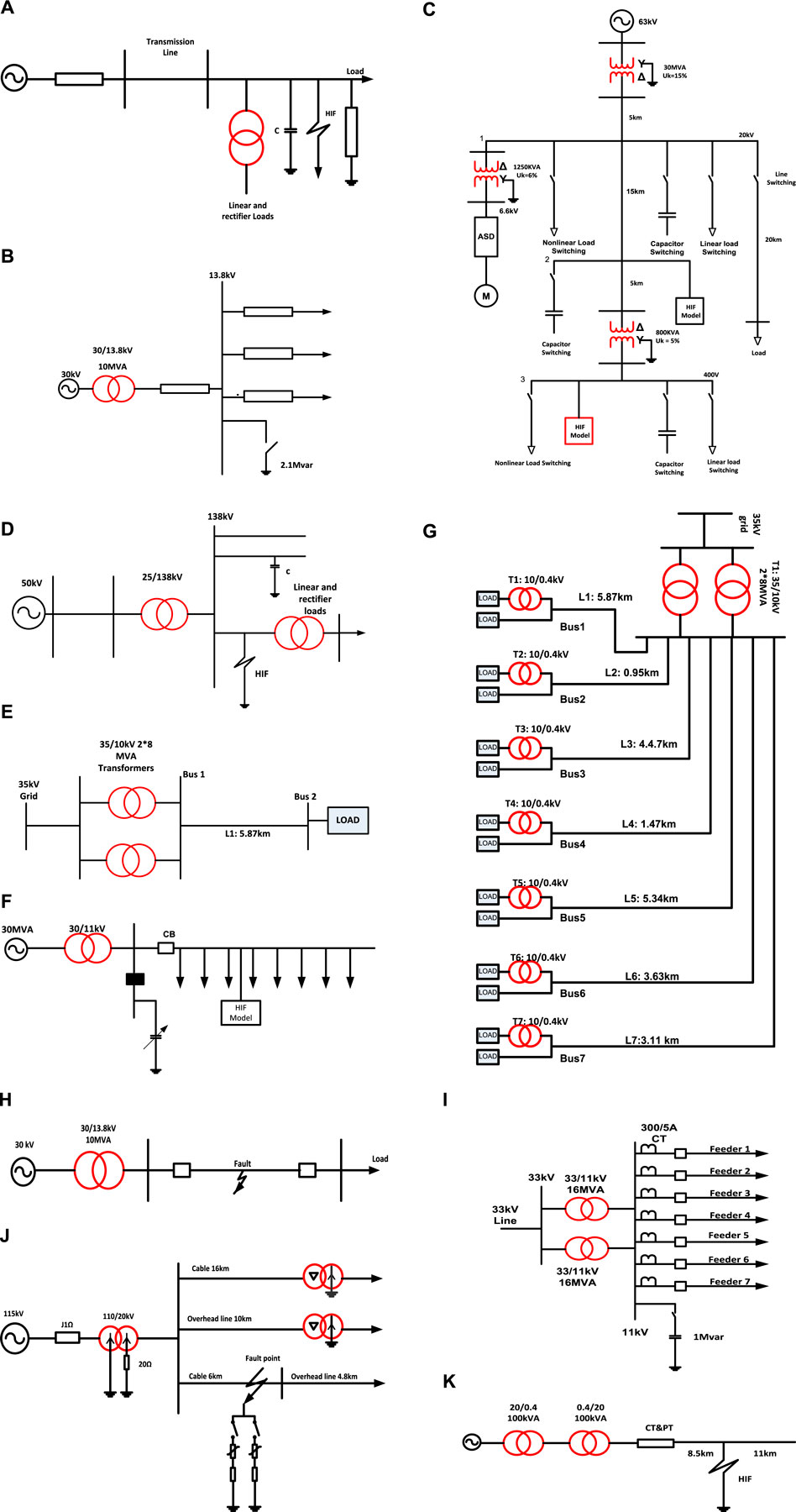
FIGURE 4. (Continued)
Vahidi et al. (2010) used the DWT technique to extract the features, and ANN classifies the faulty cases with other power system disturbances. A three-phase radial distribution network is modeled using the PSCAD/EMTDC software used as the test system. The power system frequency is 50 Hz, and the power is supplied at 63 kV from a 30-MVA transformer (wye/delta). The transformers and line parameters are shown in Figure 4C. Line currents during the HIF have high-frequency components and are used for feature extraction. The extracted features are decomposed into two levels of detailed and approximation coefficients at six cycles. The performance of the DWT-based denoising technique depends on the threshold value
The system tested by Tawafan et al. (2012) is a 115-kV distribution feeder comprised of a substation, and three radial network distribution feeders are shown in Figure 4B. The generator is 30 kV and 10 MV connected to the 30/13.8-kV and 10-MV transformers. The 6-pulse rectifier is used for the representation of the non-linear load. The simulation models are created using PSCAD, and the sampling rate is 15.36 kHz. FFT is the feature extraction technique used, with an algorithm based on the adaptive neural Takagi–Sugeno–Kang (TSK) fuzzy modeling scheme, where the HIF detection is performed by taking the amplitude of the ratio of the second and odd harmonics to fundamental harmonics of the current signals that serve as input to ANFIS. The fundamental harmonics are decreased when the fault has occurred. A total of 570 cases are taken, among which 138 cases are HIFs and 432 are non-HIFs. The mean squared error value of the model is 0.1163, and based on the output of ANFIS, if the HIF current is greater than 0.6 it indicates HIF conditions and if it is less than 0.4; it is non-HIF conditions. The detection accuracy of HIF cases is 97.8%, and non-HIFs is 99%. The method was proposed by Soheili et al. (2018). The harmonic components of the third, fifth, seventh, eleventh, and thirteenth HIF current are preprocessed in an EKF, and 12 features are extracted. These features of one-, two-, and three-cycle windows are considered the input to train the RF. RF is trained with 20,580 and 8,820 data sets. The SNR chosen is 20 dB. Two separate, three-phase sources are connected through transformers to a transmission line of length 100 km. The transmission lines are 138 kV, and the transformers are 50 MVA, supplying at 138/25 kV to the distribution network (Figure 4D).
The distribution feeders (pi sections of 20 km each) work at 25 kV and are connected with shunt capacitors, linear loads, and a 2-MVA 6-pulse rectifier load (non-linear load). The resistance, inductance, and capacitance of positive and zero sequences of transmission lines are as follows: R1 = 0.01273 Ω/km, X1 = 0.9337 mH/km, C1 = 0.0012 lF/km and R0 = 0.3864 Ω/km, X0 = 4.1264 mH/km, and C0 = 0.0075 lF/km, respectively. The resistance, inductance, and capacitance of distribution lines (pi-section) are R1 = 0.2568 Ω/km, X1 = 2.0 mH/km, and C1 = 0.0086, respectively. The total percentage impedance of the transformers is 6.75%. The simulation models are developed using PSCAD (EMTDC), and the sampling rate chosen is 1.0 kHz on a 50-Hz base frequency (20 samples per cycle). RF proved to be the best, with 93.56% accuracy and 94.56% dependability. A multi-feeder radial distribution system was proposed by Sarwagya et al. (2018) to detect and segregate HIFs. It consists of a 30-MVA, 33-kV substation, and five numbers of 11 kV radial distribution feeders. The positive-sequence impedance of the distribution line is 0.3 + j0.25 Ω/km. The discrimination of the HIF is performed based on two criteria. The first is based on the maximum value of the one-cycle sum of superimposed components of negative-sequence current for faulty feeder identification, and the second is based on the one-cycle sum of superimposed components of residual voltage for HIF detection. The substation bus provides the residual voltage. The negative sequence current of all the feeders is compared, and the maximum value of the negative sequence will be for the feeder where HIF has occurred. The HIF is accurately detected in 3 s with the proposed method. The performance of the method with HIF during unbalanced loading, unbalanced loading conditions, capacitor switching, and occurrence of an HIF in various feeders is analyzed. Sarlak and Shahrtash (2011) compared two approaches for HIF identification: the voltage phase difference algorithm and a combination of DWT and ANN. The test system chosen is from Bosnia and Herzegovina, a distribution system like in Europe. The article includes two test systems: a two-bus feeder system and the other is an eight-bus system. The two-bus system is a simple one with a main transformer of 35/10 kV, whereas the latter one is more complex, consisting of 8 feeders fed from 35/10 kV, with underground cables and a transformer at the end consumers rating at 10/0.4 kV. Figures 4E, G represent two- and eight-bus systems, respectively. The sampling frequency is 3.2 kHz. The first method DWT is applied to the measured voltage signals. Each voltage has four detailed coefficients and one approximation coefficient. An algorithm is proposed in which DWT signals are combined, representing a signature for symmetrical and unsymmetrical faults. These data are then used to train and test the ANN. A total of 1,600 cases are simulated, including non-faulty conditions and three types of fault conditions. The method gives an accuracy of 100% for the 20–600 Ω range of fault resistances and at different fault locations. In the second method, a voltage measurement is performed, and the Hilbert transform is applied to obtain the best features. The best feature is an instantaneous frequency, which represents the time rate of change of the instantaneous phase angle. The phase difference is calculated by the difference between the instantaneous phases of voltage signals. The voltage phase difference algorithm calculates the PD during normal and fault conditions. At normal working operation, the phase difference will be 1200, and during each fault condition, the phase difference will be different. This parameter is used to detect and classify the fault. With 2,000 cases in two-bus systems, the accuracy obtained is 92.5%, whereas the eight-bus system showed 90.19%. Panigrahi et al. (2018) used the IEEE Power System Relaying Committee Working Group at medium voltage levels. A simple 11-kV radial distribution feeder with eight nodes is shown in Figure 4F. MATLAB/SIMULINK program is selected and modeled, and the line impedance (positive sequence) is chosen as 0.3 Ω/km + j 0.25 Ω/km. At a distance of 5 km, nodes are isolated from each other, in which nodes 1, 3, 5, and 7 are connected to linear capacity loads of 1 MVA each at power factor 0.9/phase, and nodes 2, 4, 6, and 8 are linked to linear capacity loads of 2 MVA each at power factor 0.9/phase. The method discussed the MM gradient for HIF detection and classified HIF, LIF, capacitor switching, and load switching (balanced and unbalanced).
The proposed method measures the three-phase voltage at a relay location and evaluates the residual voltage. The morphology gradient is used to extract the irregularities in the voltage signal. The extracted feature index is determined from the zero-energy index at NC and compared with a predefined threshold value. The extracted feature index value will jump slightly for HIF, LIF, and other disturbances for faulty conditions. An HIF is created at nodes 1, 4, and 9, and the occurrence will be for 1 s. The method accurately detects HIF occurrence in 0.8 s. The test system model proposed by Wali et al. (2018) is a 13.8-kV radial distribution feeder simulated by MATLAB/SIMULINK under different scenarios, such as linear load, non-linear load, and several other conditions. Figure 4H shows a single-line representation, a three-phase transformer, and a 13.8-kV distribution network. The non-linear load is represented by a 6-pulse rectifier that creates non-linear features in the feeder. The method used for HIF detection is FFT for feature extraction, and the power spectrum technique is used to identify the fault, which gives an accuracy rate of 100%, the time required is less, and that does not require any level of training. FFT extracts the feature of the current signal from the faulty feeder, and the power spectrum of the time signal is determined using the function FFT. If PS is less than 0.005, then a HIF occurs. HIF of 250 cases and other power system disturbances of 750 cases have been analyzed in this study. The method distinguishes events due to capacitor banks, non-linear loads, linear loads, and HIF.
The test system used for HIF detection (Veerasamy et al., 2018) consists of a grid source of 50 MVA/30 kV, a distribution transformer (12 MVA, 30 kV/13.8 kV), a common bus of 13.8 kV, and five radial type distribution feeders, integrated into the load facility. An Emanuel two-diode model consisting of two variable DC voltage sources of 1–10 kV connected to anti-parallel diodes by non-linear resistors of 50–500 Ω is considered an HIF model with non-linear arc characteristics. The method is proposed by extracting the features using CWT and DWT and classifying the extracted features by ANFIS. CWT gives the region at which the fault has occurred, and DWT can locate it by calculating the standard deviation (SD) using a five-level decomposition. The extracted SD values of different fault conditions with different values of fault resistance from the detailed and approximation coefficients are obtained, which are used to train classifiers FLS and ANFIS. Various faults, such as symmetrical, unsymmetrical, and HIFs, were tested using MATLAB/SIMULINK. The classification rate of ANFIS is 100%, which proved more effective than FLS. Wang et al. (2018) proposed that an HIF detection algorithm identifies the non-linear voltage–current characteristic profiles (VCCP) for identifying an HIF in the MV distribution system. During HIF, the zero-sequence current is less than the positive-sequence current. The slope of the VCCP is the numerical difference between voltage data from current sample data, and the least square linear fitting method is proposed. The wavelet correlation coefficient (WCC) is considered to improve the reliability of the algorithm. If WCC is greater than 0.966, the metered data are from a faulty feeder, and if less than the value, it is a healthy feeder. The radial distribution system is the test system in Figure 4J that uses EMTP/ATP program. The typical Mayr arc model is simulated and drawn in series with constant resistance using a switcher and parallel branches. The simulation time stage was set at 2 μs field-metered data from KEPCo, South Korea, and HIF experiments were performed on a 22.9-kV no-load overhead feeder to check the simulations. As it is a no-load feeder, the zero-sequence current and phase voltage were used at a faulty feeder outlet to correctly estimate the fault point voltage and fault branch current. The faults have been tested on various dry surfaces. The algorithm showed excellent results in real-time digital simulator tests. The test system proposed by Sedighi et al. (2005b) for HIF tests and data collection is a radial feeder of 20 kV at Qeshm Island, Iran, as shown in Figure 4K. The feeder is energized from another 20-kV feeder by two distribution transformers (20/0.4 kV, 100 kV A) connected back-to-back. The HV and LV connections of the transformers are delta/star connected. The HV sides of the transformers are connected to feeders, and the LV sides are connected to the low-voltage switch. Three-phase voltages and currents were monitored and recorded using Hall effect current transformers, potential transformers (PT), power analyzers, and computers. The sampling rate of the recorded data was 24,670 kHz for each test, and the overall recorded time was 15 s. The method used for HIF detection uses WT for feature extraction with a three-level decomposition of current signals. The first method uses GA for feature vector reduction, and the Bayes classifier is used for classification. In the first method, coefficients of three-level decomposition are used for feature extraction. They are divided into 10, 5, and 5 segments. In GA, each segment is mapped to a 20-dimensional space. A space with 20 dimensions is mapped to a space with five dimensions. The Bayes classifier is used to classify the mapped space. In the second method, WT transforms are also applied for the current signals, PCA is used for feature vector reduction, and NN is the classifier. The coefficients of three-level decomposition are used for feature extraction, divided into 10, 5, and 5 segments. Means of the absolute value of each segment were chosen as features, and the extracted signals were mapped to a 20-dimensional space. Using PCA, space was reduced to a 7-dimensional space. A perceptron NN using backpropagation discriminates between HIF, isolator leakage current, and other power system transients. Sekar and Mohanty (2020) stated that morphology gradient extracts the features of which a rule is set by RF and then fed to a fuzzy rule-based algorithm for HIF detection. The electric power distribution system (EPDS) was modeled using MATLAB/SIMULINK. A three-phase shunt capacitor of 1 Mvar has been connected to the busbar to improve power quality and output. The inrush current of a transformer produces an asymmetrical current signal that may serve as a transient signal generated by switching that may be like the HIF current waveform. An induction motor is connected as a load to study the motor operation impacts. The EPDS uses linear and non-linear loads to simulate the loading scenario, as shown in Figure 4I. One cycle window length of the current signal is measured, the impulsive feature of the signal is extracted, and a rule set is created from the statistical features of RF. The sampling frequency is 1,000 Hz, and the signal length is 0.5 s. The periodic signal has third- and fifth-order harmonics, and other harmonics that are negligible make the filter closer to HIF detection. The method effectively detects an HIF from other power system disturbances.
3.2 Mesh distribution network
The test system proposed by Lai et al. (2005) consists of two 50 MVA generators with 25 kV lines, two transformers, and linear and non-linear loads. In DWT, db4 was chosen as the mother wavelet, with a downsampling frequency chosen as 9,600 Hz, used to extract the detailed and approximation coefficients from the signals of the HIF and non-fault. The current and voltage signals at a targeted circuit breaker are measured. The RMS values of the measured quantities at various frequencies are analyzed and given as input to the nearest neighbor to classify fault signals. The HIF and non-HIF cases (1,000 cases each) were simulated with HIF and LIF models. The range of total error corresponding to the RMS value of the voltage wavelet coefficient is from 2.52% to 45.4% and will not indicate the physical properties of the output coefficient.
Samantaray et al. (2008) reported that S transform and TT extract the features, and FNN and PNN classify the faulty and non-faulty conditions of the HIF. The ST features are extracted from the HIF and normal fault current signals for half-cycle current signals after fault inception. The energy and SD of time and frequency information are considered feature sets. These features are used to train and test the FNN for radial and mesh networks. TT transform also extracts energy and SD of the TT-counter and time index after fault inception for the first half-cycle of the fault current. A total of 500 cases are simulated for training and testing the classifier. The system is modeled in MATLAB/SIMULINK, and the sampling rate chosen is 1 kHz. The PNN classification is based on the distribution values of the probability density function. The classification rate of a radial network with PNN using ST features is up to 98.06%. PNN with TT transform features gives a classification rate of up to 98.05%. The accuracy of the FNN and S transform combination is 93.04%, and the accuracy of the TT transform is 94.16%. The proposed method is also tested in a mesh network. The accuracy of the mesh network with S transform and FNN is 92.86%, and that with TT transform and FNN is 93.55%. The S transform and PNN combination gives 97.85% accuracy, and the TT transform and PNN combination gives 97.09% accuracy.
The HIF detection method used by Samantaray et al. (2009a) is a combination of AEKF with FNN and PNN. The schematic diagram of the test system chosen is given in Figure 5. The base voltage of the distribution network is 25 kV, and the generator is 10 MVA, 15 kV capacity. The harmonic components estimated by the AEKF are fundamental, third, fifth, seventh, eleventh, and thirteenth harmonics for the HIF and NF under non-linear loads. The AEKF calculates the harmonic component within half a cycle of the fault occurrence, with the peak of the estimated harmonic component considered that inputs to PNN and FNN. The PNN classification is based on the probability density function’s distribution values. PNN is analyzed using a data set with an SNR of 20 dB, 300 data sets for training, and 200 data sets for testing. For the classification, PNN takes 0.1 s time, whereas FNN takes 0.2 s. Fault and non-fault conditions with non-linear switching (a six-pulse rectifier is used) are checked using various models of MATLAB/SIMULINK, and the sampling rate chosen is 1.6 kHz. The accuracy rate of PNN is 99.11% compared with FNN having 96.51%.
The detection of HIF described by Routray et al. (2016) uses a test system with a generator of 50 MVA supplying 138 KV of voltage to the utility sector through a transmission line 100 km long, and a 138/25-kV star/delta transformer is considered for testing the method. The method uses ST for feature extraction and ANN for discriminating the HIF with load switching, capacitor switching, and NC. The time and frequency information is extracted from the S matrix, and the amplitude factor is calculated from current signals. A total of 4,010 cases were considered, of which 60% is used for training and 40% for testing. The overall accuracy of classifiers for normal fault is 98.75%, 96.4%, 94.06%, and 92.60% for normal (without noise) and noisy conditions.
Samantaray (2012) studies two test systems: one with a radial feeder mentioned in Figure 5 and the other with a mesh feeder given in Figure 7C. The test system studied is connected to a 50-MVA generator and a transformer of 138/25 kV from a transmission line of 138 kV and a length of 100 km. Loads are connected with linear and non-linear loads. The resistance, inductance, and capacitance of positive and zero sequences of transmission lines are R1 = 0.01273 Ω/km, X1 = 0.9337 mH/km, C1 = 0.0012 lF/km and R0 = 0.3864 Ω/km, X0 = 4.1264 mH/km, and C0 = 0.0075 lF/km, respectively. The resistance, inductance, and capacitance of distribution lines (pi-section) are R1 = 0.2568 Ω/km, X1 = 2.0 mH/km, and C1 = 0.0086, respectively. The total percentage impedance of the transformers is 6.75%. The simulation models are developed using PSCAD (EMTDC), and the sampling rate chosen is 1.0 kHz on a 50-Hz base frequency (20 samples per cycle). RF proved to be the best, with 93.56% accuracy and 94.56% dependability. On the distribution feeder, the HIF faults are generated at 25 kV, 20 km, pi section. Different simulation conditions are also considered, such as three-phase loadings, single-phase loadings, transformer energizations, shunt capacitor switching, and HIF by varying DC voltage sources. Two combinations of the HIF detection technique are proposed: the first is an EKF and RF and the latter is DT with FFT. The harmonic components of the third, fifth, seventh, eleventh, and thirteenth HIF current are preprocessed in an EKF, and 12 features are extracted. These features of one-, two-, and three-cycle windows are considered in this work. Considering the two-cycle window and with SNR set at 20 db. The simulation models are developed using PSCAD (EMTDC), and the sampling rate chosen is 1.0 kHz. RF is trained with 20,580 data sets, and 8,820 data sets are tested. RF proved to be the best, with 93.56% accuracy and 94.56% dependability compared with DT.
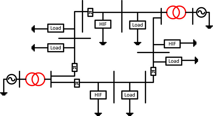
FIGURE 5. Three-phase meshed network.
Mishra et al. (2016) used S transform with ANN and SVM to discriminate the HIF from other power system disturbances. A total of 4,000 cases, including HIF, normal, load switching, capacitor switching, and normal faults, are taken. Features are extracted from three-phase currents measured from the bus, and the best feature vector is selected. MLPNN with backpropagation NN and SVM along with ST is used, with 60% data for training and 40% for testing. The distribution model with a radial pattern of a 50-MVA generator is connected to a 100-km-long transmission line and a 138/25-kV star/delta transformer to supply 138 kV voltage to the utility sector. For the ideal case, ST with ANN and ST with SVM give 100% accuracy, whereas with SNR 30 dB, ST with ANN gives 93.7% and ST with SVM gives 92.15% accuracy. For the ideal case with the mesh network, ST with ANN and ST with SVM give 100% accuracy, whereas with SNR 30 dB, ST with ANN gives 81% and ST with SVM gives 86% accuracy.
3.3 Palash feeder, Tehran
Detection of the HIF using a combination of MLPNN based on multi-resolution morphological gradient features of the current waveform is described by Sarlak and Shahrtash (2011). The MMG features of the current signals (for three half-cycles) of broken and unbroken conductors are considered, and the features from DFT, DTT, DST, and DWT are compared. The morphology gradient is the difference between the dilation and erosion functions. Data acquisition is performed using the ION7650 meter, and the input port of the meters is connected to the outputs of the current transformers at the 63/20-kV substation. The sampling rate of the current waveform is 1.6 kHz. A disturbance detection module is based on MMG-extracted features of any subwindow with a predefined threshold. Three MLPNNs (A, B, and C) are trained individually by applying the time-based features obtained from the first, second, and third sub-windows. Then, their decisions are concatenated to make the final decision. The proposed algorithm gives security of 96.3% and dependability of 98.3%.
Nikoofekr et al. (2013) used a test system from Tehran, Iran, which has a 63/20-kV transformer feeder with 30 MVA apparent power, and the HV side has been grounded with a zigzag transformer and variable resistance adjusted at 29.5 Ω. Moreover, two 2.4-MVAR capacitor banks are connected through the HV circuit breakers. The ION 7,650-meter tests the HIF current and non-HIF current signals, such as insulator leakage current (ILC) and harmonic load current, with a sampling rate of 64 samples per cycle at the site. The method uses ST for phase correction in CWT, which localizes the phase and amplitude spectrum. TT transform extracts the features of the measured signals. Five different ART neural networks are used to classify the HIF and tested with broken conductors in asphalt, concrete, gravel surfaces and unbroken conductor on trees and under no fault conditions. This study uses five types of ART networks, namely, ART1, ART2, ART2-A, Fuzzy ART, and Fuzzy ARTMAP. The different features extracted were energy, SD, and median absolute deviation. The performance of the ART network is based on the vigilance parameter
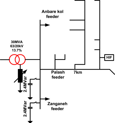
FIGURE 6. Palash feeder single-line diagram.
MMG is the feature extraction used by Sarlak and Shahrtash (2013) and tested on the Palash feeder in the Southwestern Tehran distribution network, as shown in Figure 6. An HIF indicator is installed in various poles that detect HIF at various locations. The HIF indicators are installed in the feeder based on the processing of the magnetic-field strength signal. The fitness evaluation combines three goals: accuracy, number of training samples, and the weighting factor. The impulse response of magnetic response in the frequency domain is calculated in terms of the electric hertz vector. By simulation, a 978-feature vector for the HIF and 852 non-HIF is calculated. The dependability and security of the proposed system are best above the 20 db SNR. To evaluate the proposed method, MMG extracts a magnetic field strength signal, which is given to SVM for classification. The proposed algorithm has 96.9% security and 97.2% dependability.
The real-time experiments are performed in the Palash feeder, Tehran (Soheili et al., 2018). The modified FFT approach is used to detect the HIF concerning non-linear loads. In the proposed method, the measured three-phase current is analyzed by FFT. These currents are continuously monitored for non-linear loads, abnormal conditions, and HIF detection. HIF currents during non-linear loading conditions and different ground types are recorded. The proposed algorithm has divided the output into three levels: 0, 0.5, and 1. NC, pickup, and HIF, respectively, are represented by these levels. Various scenarios in the simulated data are considered, including high current three-phase feeder, low current three-phase feeder, low current single-phase feeder, and capacitor switching events. The distribution network is energized via a 63-kV/20-kV three-phase transformer with a rated power of 30 MVA. Data recording has been conducted using the ION 7650, with a sampling rate of 64 samples per cycle (3.2 kHz). The various surfaces where real-time experiments are conducted are concrete with 20 cm in no-load conditions, concrete with 10 cm in 55% full load conditions, and asphalt with 2 cm under 55% full load conditions. The HIF detection time of the proposed method was 1.13 s.
3.4 IEEE test systems
There are various IEEE test systems, such as the single-line diagram of the IEEE 13-node system (Figure 7A), the single-line representation of the IEEE four-node test system (Figure 7B), the IEEE-123 distribution feeder (Figure 7C), and the IEEE 34-node test system (Figure 7D).
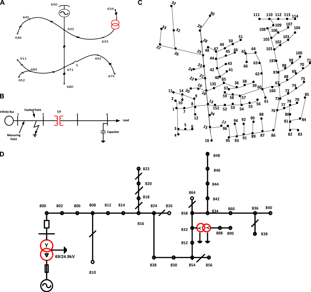
FIGURE 7. (A) Single-line diagram of the IEEE 13-node system. (B) Single-line representation of the IEEE four-node test system. (C) IEEE-123 distribution feeder. (D) IEEE 34-node test system.
3.4.1 IEEE 13-node systems
The illustration given by Gautam and Brahma (2013) used an HIF detection tool using MM that can be implemented along with the conventional overcurrent relays in the substation. Both IEEE 13- and IEEE 34-node test feeders are used to validate the approach. Closing Opening Difference Operation effectively detects a disturbance in waveforms. A low sampling rate of 3,840 Hz (64 samples per cycle) was chosen to reduce computing time. The dilation and erosion function of MM and its difference will effectively detect the disturbance in the waveform. Voltage waveforms measured at substations are used in the procedure. The fault detection time is less than 1 s, and the method is fast and reliable. The two-test system gives 100% accuracy in detecting and classifying unbroken, broken conductors, capacitor switching, and load switching. A modified FFT approach based on HIF detection is proposed by Soheili et al. (2018), in which non-linear loading conditions are also considered. At node 630 of the IEEE 13-node system, the type of feeder, point of common coupling (PCC), and the current rate are considered, and the recording devices are installed at this node to resemble the real-world scenario. The feeder connected between 650 and 632 is considered the three-phase high current feeder with 300 A, 606 m long. The feeder between 692 and 675 is considered a low-current three-phase feeder with 80 A. The main factors considered include high and low three-phase currents and low current single-phase feeders. The scheme successfully distinguishes the HIF with load switching and capacitor bank switching in 1.15 s. Wang et al. (2019) used variational mode decomposition (VMD) and Teager–Kaiser energy operators (TKEOs) to identify the HIF. The method is tested in radial, IEEE 13-node, IEEE 34-node, and test microgrid systems, as well as experimental field tests. Three-phase current signals are measured, and VMD is performed on transient zero sequence currents (TZSCs) to obtain the intrinsic mode functions (IMFs). Then, the IMFs with the largest kurtosis value were selected as the characteristic IMFs. Second, the characteristic IMFs are calculated to obtain TKEOs and divided into subintervals of TKEOs waveform to calculate the time entropy values. The HIF detection criterion is when the time entropy value is 0; then, CS or LS has occurred. When the entropy value is not 0, it is judged as an HIF. The calculation time taken is 0.0028 s.
A data-driven technique includes PCA, Fisher discriminant analysis, and binary and multi-class SVM for HIF detection. Compared with PCA, FDA can classify and locate the HIF successfully (Sarwar et al., 2020). PCA utilizes Hotelling’s T2 statics for HIF discrimination (see Eq. 1). The IEEE 13-node system is used for testing:
where Fα (m, n-m) is the F distribution with m; (n–m) is the degree of freedom; T2 ≤ T2 α means no-fault condition; and T2 > T2 α means faulty condition.
The SVM uses a discriminant function to differentiate various classes. Non-linear classification is based on a kernel function from kernelized SVM. Figure 7A shows the single-line diagram of the IEEE 13-node system. Multiclass SVM gives the best results, with dependability and security at 100%. Silva et al. (2020) performed a wavelet packet-based feature extraction with a three-level decomposition of signals at 2.5 kHz along with the EuFNN classifier. The IEEE 13-bus system is considered for testing the method, which is a highly charged compact feeder with a rating of 4,053 kV A and a power factor of 0.85, and an extension of approximately 1.5 km from bus 650 to bus 680. Several line configurations, such as three-phase and single-phase lines, overhead, and underground sections, are considered. Different families of wavelet transform, namely, Haar, Symlet, Daubechies, Biorthogonal, and Coiflet, used to extract features from a one-cycle time window of current signals were chosen. The RMS and the entropy values calculated for Daubechie-8 give the best discrimination rate. Various WPT families, the MLP, learning vector quantization (LVQ), SVM, and EFuNN classifiers were compared, among which MLPNN gave the least accuracy, and all other classifiers gave an average of 97.14% accuracy. Nezamzadeh-Ejieh and Sadeghkhani (2020) performed the time-domain HIF detection algorithm by analyzing the substation current employing Kullback-divergence that measures the similarity between asymmetry and non-linearity of two consequent half cycles. Both IEEE 13-node and IEEE 34-node feeders are used to test the approach. The amplitude of the fault current of 15 A is approximately 3% of the normal feeder current. An intelligent electronic device samples the signals at 4.8 kHz and measures the current in each phase. The current vector measurement is formed by
During normal operation, there is no change in the waveforms of two consecutive half-cycles DKL = 0, and during a fault occurrence, there will be asymmetry and non-linearity in the half-cycles and DKL ≠ 0. During the HIF, the third harmonic current will be greater than the fifth harmonic current. The occurrence of an HIF is when
3.4.2 IEEE 34-node test system
Moravej et al. (2015) used an IEEE 34-node test feeder for testing, as given in Figure 7D, and simulated it in EMTP-RV software. There are four different conductors, in which the system is characterized by heavily and lightly loaded with a feeder voltage of 24.9 kV. Two-line regulators and one transformer (24.9/4.16 kV) are present in the feeder. There are single-phase and three-phase feeders and two shunt capacitors in the system. Dual-tree complex wavelet transforms is used for feature extraction and PNN for classifying the faulty and healthy conditions. In the method, various steps involved in HIF detection include disturbance detection, disturbance feature extraction, HIF detection, frequency tracking, over-current protection, and the main feeder break detection. In the first step, the fundamental frequency current of the three-phase current is calculated using the DFT algorithm. The post-disturbance and pre-disturbance data windows are saved in memory, and both are decomposed into five levels by DT-CWT. The detailed components of the post-disturbance data window are subtracted from those of the pre-disturbance, and after obtaining the detailed component of the disturbance signal, the proper feature is selected. The SD and normalized energy of the detailed coefficients of level 2–level 5 three-phase currents and residual current were selected as the features for the HIF detection algorithm. The algorithm is fast and detects the disturbance in 1.88 ms, giving an accuracy of 98.88%. Sekar and Mohanty (2017) proposed that MM extracts features, such as energy, mean, and SD, which train the DT (data mining based). The three-phase current signal is pre-processed by a dilation and erosion morphological filter. The data mining-based DT using software package “R” is used, as well as post-disturbance data window length of current signals at feeder processed through the MM filter and chosen data window. The IEEE 34-node test system with light loads is also used. The total number of cases considered is 300, of which 70% are used for training and 30% for testing. The accuracy is 98.83%, dependability is 98.88%, and security is 100%, with a detection time of 30 ms. The proposed method is also tested using the IEEE 13-node system, in which the total cases considered are 300, of which 70% are used for training and 30% for testing. The accuracy is 98.83%, dependability is 98.88%, and security is 100%, with a detection time of 30 ms.
Fan and Yin (2019) used a convolutional neural network and transfer learning-based approach for HIF detection. The method is tested with 5,000 data sets, of which 2,500 are HIF data and 2,500 are non-HIF conditions in an IEEE 34-node feeder. From the data set, 80% was taken for training and 20% for testing. The sampling rate was 15 kHz, and there were 300 samples in the input data. Among the four layers of the CNN, each layer of the CNN model has convolution, rectified linear unit (ReLU), and max-pooling functions. The accuracy of the CNN obtained was 99.52%, and the computational cost was low compared with the traditional MLPNN (91.13%). Fewer data sets (<300) were in the IEEE 13-node system with 50% training and 50% testing data. The accuracy obtained for the CNN was 95.06% compared to CNNs, with 74.69%.
3.4.3 IEEE four-node test feeder
The test system used is the IEEE four-node system, as shown in Figure 7B. Three-phase load switching, capacitor switching, no-load transformer switching (energizing and de-energizing the transformer at various cycle times), harmonic loads (e.g., an unregulated four-pulse rectifier and induction motors), arc furnaces, and down-conductor and undowned conductor HIFs are discriminated using this method. The method of HIF detection (Sarlak and Shahrtash, 2008) uses PCA and LDA and is used along with SVM to detect the HIF, which gives 97.5% accuracy. PCA refers to the linear feature extraction method that computes m eigenvectors corresponding to n-dimensional patterns. PCA extracts uncorrelated features. Hence, it is more appropriate compared to other classification techniques. LDA measures the Fisher criterion that finds the m eigenvectors of the scatter matrix that discriminates HIFs from non-HIFs. The extracted features are sampled at the rate of 12.5 kHz. The feature set is divided into a training set of 66% and a testing set of 34%. The polynomial and radial bias function of SVM is used, in which the linear kernel function has the best classification accuracy.
3.4.4 IEEE-123 distribution feeder
An IEEE-123 distribution feeder as a test system is illustrated, characterized by unbalanced phases modeled with EMTP-RV software. Figure 7D displays the IEEE-123 distribution feeder. Some of the feeder buses are connected to smart meters in three-phase sections and not in single- and two-phase sections. Tonelli-Neto et al. (2017) found that the method uses WT along with ANN and fuzzy interference systems for HIF detection. Three-phase current signals are analyzed and sampled at a frequency of 15.36 kHz. An application of DWT, multi-resolution analysis extracts the features from the current signals using Daubechies mother wavelet with fourth-order filter (db4). An energy concept is applied to the features to increase efficiency and minimize the number of coefficients. The energy concept is used for the third-level detail coefficients because of the high number of coefficients created in MRA. Fuzzy ARTMAP neural networks and fuzzy interface systems are used for HIF classification. Each bus, where the signals are obtained, has a FIS responsible for identifying and qualifying the feeder operating condition in the detection based on FIS. The results combine a normal case, HIF phase a, HIF phase b, and HIF phase c. The detection method based on the fuzzy art neural network (FANN) is as follows: the vectors obtained are normalized for use as inputs to multiple neural networks. This normalization is performed by identifying the maximum current value of each analyzed vector. Comparing both FANN and FIS, the accuracy of FANN is 97.69%, and that of FIS is 99.25%.
3.5 Test microgrid system
The test microgrid system is used for HIF detection (Kar and Samantaray, 2017), as shown in Figure 8A. The base power of the test system is chosen as 10 MVA. The rated short-circuit of the utility is 1,000 MVA with f = 60 Hz, rated 120 kV. Distribution generations, DG1 and DG3, are rated as follows: synchronous generator rated at 9 MW and rated voltage of 2.4 kV, and DG2 is a wind farm consisting of three wind turbines (2 MW each), rated kV = 575 V. The transformer ratings used in this study are as follows: Transformer 1: 15 MVA, 120/25 kV. Transformers 2 and 4 are rated at 12, kV = 2.4 kV/25 kV, while Transformer 3 is rated at 2.5, kV = 575 V/25 kV. The distribution lines (DL) are DL1, DL2, DL3, and DL4: PI-Section, 20 km each. The total load is 20 MW, 10 MVAR, a sum of L1–L5. The MODWT is the feature extraction technique, and DT is the classifier used. The proposed method is tested in both grid-connected and islanded modes. The MODWT scaling filter and the wavelet filter related to the DWT filter are calculated, and the scaling coefficients of MODWT are obtained. The detailed approximation coefficient is obtained from the MODWT, and DT does accurate classification. The total cases are 1,493, of which 973 are HIF cases and 520 are faulty conditions. In the method proposed, 12 feature sets are considered, among which five were taken for classification. The training set (70%) and testing (30%) assess the performance. The software package “R” generates data mining for the DT. The detection accuracy, dependability, and security are 100% for the grid-connected mode, whereas for the islanded mode, the accuracy is 99.23%, security is 98.23%, and dependability is 100%.
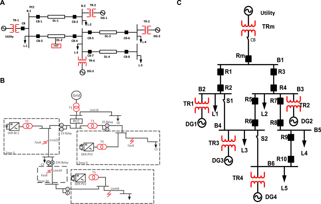
FIGURE 8. (A) Test microgrid system. (B) Representation of CERTS microgrid system structure. (C) Single-line representation of IEC microgrid.
Microgrid is considered while integrating distributed energy systems (Abdelgayed et al., 2017). The Consortium for Electric Reliability Technology Solutions (CERTS) was used for the case study of microgrids in this article. The microgrid system has two modes of operation: grid-connected and islanded mode of operation. CERTS microgrid consists of a distribution system fed from three-phase distribution transformers rated at 13.8/0.48 kV, consisting of two solar photovoltaic sources and one battery energy storage source. Four loads are considered long in the distribution system. The method employs a semi-supervised machine learning strategy to handle labeled and unlabeled data. DWT extracts the hidden properties of voltage and current and applies them to a harmony search algorithm to find the HIF parameters. The DT and KNN classifiers are used to discriminate the HIF events. The overall accuracy of the DT is 100%, and that of the KNN is 95%.
The test system is a CERTS microgrid with two inverter-interfaced DG units and one synchronous generator-based DG unit (Gadanayak and Mallick, 2019). The representation CERT microgrid system is shown in Figure 8B. For HIF detection, the test system consists of five distribution lines and five relay units. MATLAB-SIMULINK is used to simulate the model, with a simulation sampling rate of 0.5 MHz. The MODWT approach for feature extraction and knot-based empirical mode decomposition is included in the methodology. The program recognized 855 cases of HIFs and 801 cases of non-HIFs. The average time to detect a fault was 0.12175 s. The test system used by Gashteroodkhani et al. (2020) was performed in a 25-kV IEC standard microgrid that gave high accuracy and robustness in noisy environments. The single-line representation of the IEC microgrid is represented in Figure 8C. A deep-belief neural network with TT-transform is employed where an intelligent relaying scheme-based real-time digital simulator is used, integrated with MATLAB. The process involves the measurement of three-phase currents at both ends and the feature extraction by Clark’s transformation and TTT, which is sent to the DBNN. Six features are used for feature extraction, including energy, SD, and median absolute deviation. Microgrid models with grid-connected, islanded, radial, and mesh topologies are used to test the approach. With 3,600 fault situations and 3,125 no-fault cases, the sampling rate was set to 1.2 kHz. The proposed method gives 99.74% and 99.46% accuracy for a radial network with grid-connected and islanded modes, respectively, and 100% for mesh topology in both modes of operation.
3.6 JMARTY model test system
Eldin et al. (2007) considered the JMARTY model with Egyptian transmission line parameters, such as a transmission line length of 125 km and a resistive load of 600 MW, as shown in Figure 9A. DWT’s feature extraction technique with classifier moving window pattern recognition is used in HIF detection in extra-high voltage transmission. The sampling rate is 250 samples/cycle at 50 Hz. In order to distinguish HIF from non-HIF events, the proposed technique uses high-frequency information from wavelet analysis db4. The effect of fault location, fault interception angle, fault type, switching of loads, switching of the HIF, and sudden load rejection is studied. The algorithm can be added to the existing digital relay microprocessor; it is fast, accurate, and simple.
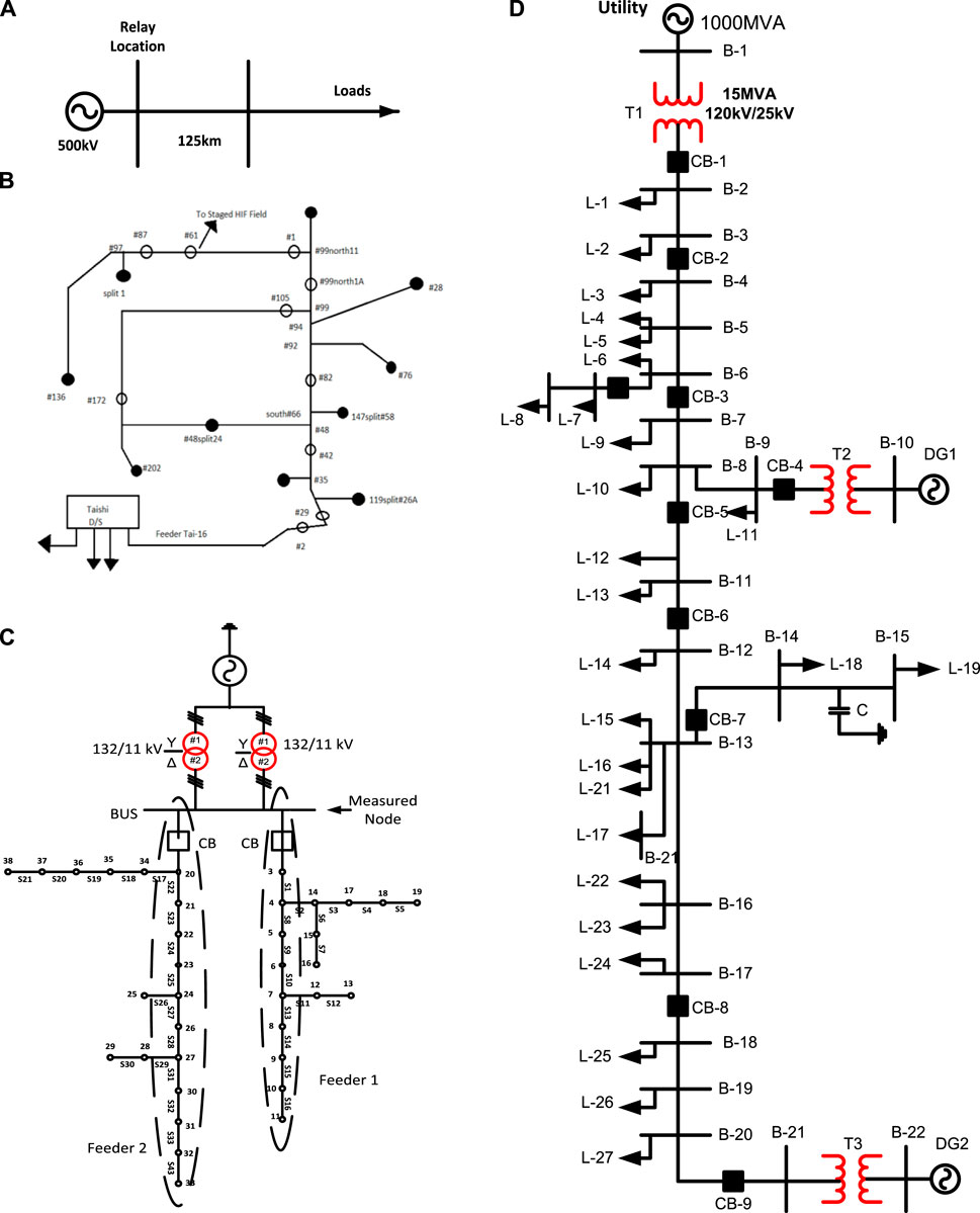
FIGURE 9. (A) Single-line representation of the JMARTY model transmission line test system. (B) Single-line representation of TAI-16 feeder distribution networks. (C) Single-line diagram of the 38-node test system. (D) Single-line representation of the benchmark system.
Ibrahim et al. (2008) described two approaches: the first uses DWT analysis and the second analyses three-phase voltages using a high-frequency tap coupling capacitor voltage transformer. The chosen sampling rate is 20,000 Hz. A 100-m-long 345-kV double-end transmission line system is considered. The effect of fault location, fault type, fault interception angle, switching of loads, and switching of HIF are studied. The method is independent of load variations and unbalanced conditions. The algorithm is fast, accurate, and simple; it can be added to an existing digital relay microprocessor (Eldin et al., 2007).
3.7 TAI-16 feeder
In Yang et al.’s method (2006), the HIF was tested in a real-time Tai-16 feeder, Taishi substation near Mailiao, as shown in Figure 9B. The fault was staged at pole #61 under grounded and ungrounded conditions, with dry and wet ground conditions. Data from the Shand-Ding substation and the She-Zi substation were considered to train the NN. The analog-to-digital recorder ADX-3000 was installed to monitor the neutral line current of the faulted feeder in the substation. A cross-linked polyethylene-covered conductor, a bare copper conductor, and ACSR conductors are used. A wavelet transform and pattern recognition-based feature extraction scheme is used and applied to backpropagation ANN for HIF detection. The detection of the HIF is carried out by introducing an intelligent HIF detector applied to a neutral line current, giving an 81% detection rate. A self-tuning algorithm based on the chi-square algorithm is applied to find the variations in neural current. A statistical confidence scheme is applied for neutral current estimation. For calculating the threshold of neutral current, a 95% confidence interval is applied.
3.8 Test system—38 nodes
A typical 11-kV distribution network in Malaysia is composed of 38 nodes serving 34-line sections, as shown in Figure 9C, displaying the single-line diagram of a 132/11-kV distribution network. The test unit has a frequency of 50 Hz, with a sampling frequency of 6.4 kHz, and delivers 128 samples/cycle. The feeder bus is simulated using the PSCAD program. Ali et al. (2014) proposed that DWT-based MRA is the feature extraction technique, and a matching approach technique is used for classification in the underground distribution system. The simulation tests of the three-phase voltage signal are obtained at a measurement point using the DWT-based multi-resolution technique. The voltage signal was decomposed into 128 samples and analyzed by Daubechies fourth order of DWT. The first level of the detailed coefficient, d1, detects the HIF by observing changes in the characteristics taken from three-phase voltage data. The sum of the first-level approximation coefficients obtained from the normal cycle, known as the approximation ratio, is divided by the sum of first-level approximation coefficients obtained from the normal cycle to classify the fault:
The approximation ratio is considered for distinguishing SLGF, LLGF, LLLF, and LLF. If the ratio is less than 1 for one phase and greater for the other two phases, then an SLG fault has occurred. The three-phase ratios will be the same for LLLF. For locating the HIF, a matching technique based on the shortest distance is used. For each line section, the SD between the measured signal and the line section is computed. The summation of the detailed coefficients of voltage signals is done in three coordinate systems and represented in three-dimensional space. The SD of each section is calculated, and the average value is calculated. The average value is compared with the SD values of each section. Each section is then arranged in ascending order of its SD values, which list the possibility of a faulty section. The method successfully located the fault after four or five iterations.
3.9 Benchmark system
In Cui et al. (2017), the test system chosen is a benchmark system in a remote Canadian community with 25 kV 60 Hz, distribution feeders that serve an 11-MW load built by McGill Power Laboratory, as shown in Figure 9D. An L-G HIF at t = 0.3 s is implemented in a hybrid distribution system. The feeder’s PCC (CB-1) will collect all the data where the HIF detector is located, two DGs at locations A and B, respectively. Three types of distribution systems are also possible to model: 1) the synchronous generator (SG) system is constructed by connecting the SG to location A without DG in location B; 2) the inverter-interfaced system is connected to location B with only type 4 wind turbines at location A and without DG; and 3) the hybrid DG system has an SG connected to location A and wind turbine generators at location B. The rated voltage is 4.17 kV for the SG, and 9 MVA is the power. Three wind turbine generators provide wind power, each rated at 575 V and 2.2 MVA. The proposed method was tested in hybrid systems, and inverter-based systems are grounded, as well as ungrounded conditions. HIF and non-HIF events of 1,944 cases each have been considered for testing and training. The method proposes an algorithm to rank the effective feature sets using a signal processing technique of DFT and Kalman filtering estimation. The effective feature set is derived from information gain or entropy. The information gain of each feature is calculated, and a calculation variable is obtained. Such calculated variables are compared and then ranked for further assessment in HIF detection. By measuring the currents and voltages at the point of the common coupling, 246 electrical features are obtained. Classifiers, such as Native Bayer’s, SVM (Gaussian kernel), k-nearest neighbor (KNN), RF, and J48, are compared, among which RF and J48 proved to be the best with 99% accuracy for both.
3.10 Modeling of HIF
Researchers provide numerous HIF models because of stochastic behavior and complicated properties. In order to acquire a good representation of the HIF, it is necessary to develop a model that specifies the features and the harmonic content of the HIF. Because arcing, which has yet to be fully modeled, is involved in most HIF events, an HIF is a difficult example to model. HIFs are non-linear and asymmetric, according to some earlier studies, and random and dynamic arcing features should be used in modeling (Zamanan and Sykulski, 2014). The arc is a continuous luminous discharge of electricity in which many free electrons and ions in an insulating medium are converted into a conducting medium. The arc was first studied as a continuous luminous discharge of electricity through an insulating medium that becomes a conducting medium due to the presence of a large number of free electrons and ions. The arc was first researched about circuit breaker disruption capabilities, with arc models used to improve circuit breaker testing (Elkalashy, 2007). The Emanuel model replicates zero periods of arcing and asymmetry by connecting two DC sources anti-parallel with two diodes (see Figure 10). Variable resistors vary the fault resistance, and a voltage supply with random values mimics HIF unpredictability. Some of the other HIF models are, two-time varying series resistors with different characteristics (Nam et al., 2001), Kizilcay’s model (Zhang et al., 2016; Mishra and Panigrahi, 2019) and Matthews arc model (Gammon and Matthews, 2001).
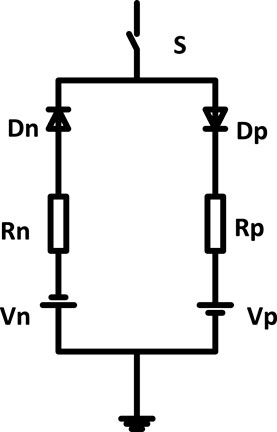
FIGURE 10. Emmanuel arc model of HIF. The Vn, Vp, Rn, and Rp values of wet sand are 4.5 V, 2.5 V, 400 ± 5 Ω, and 350 ± 5 Ω, respectively. For dry sod, the values are 4 V, 2 V, 300 ± 5 Ω, and Rp 250 ± 5 Ω. The wet grass Vn, Vp, Rn, and Rp values are 2.75 V, 1 V, 150 ± 5 Ω, and 125 ± 5 Ω, respectively. The Vn, Vp, Rn, and Rp values are 2.5 V, 0.75 V, 100 ± 5 Ω, and 75 ± 5 Ω, respectively, for reinforced concrete.
4 Classifiers for identifying the healthy and faulty conductors
This section discusses classifiers, which distinguish between faulty and non-faulty conditions. Classifiers set a boundary between healthy and faulty conductors. In the classification process, two types of data are to be considered: training data consisting of information relating to known patterns and testing data, which are a collection of information relating to unknown patterns. Table 3 presents the performance evaluation of various classifiers with various criteria, such as accuracy, dependability, security, sensibility, speed, and safety.
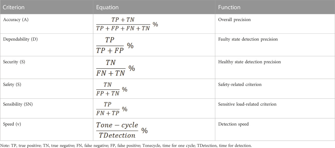
TABLE 3. Performance evaluation of classifiers.
The appropriate classifier is chosen depending on the application where it is being used. The various classification conditions are capacitor switching, load switching, noises (Christie et al., 1993), disturbances (Russell and Benner, 1995), and voltage spikes. Faulty conditions include L-L, L-G, L-L-L, LIF, HIF (Barnard and Pahwa, 1993), and non-linear load conditions (Sultan and Swift, 1992). A knowledge-based system (Sedighizadeh et al., 2010), microprocessor (Kwon et al., 1991), signature-based detection (Wester, 1998), mechanical detection (Balser et al., 1986), burst noise signals (Aucoin and Russell, 1987), and DSP were previously used in classification. Different classifiers, such as neural networks (Vyshnavi and Prasad, 2018), SVM (Mishra et al., 2016), fuzzy logic, ANN (Baqui et al., 2011), GA (Zamanan et al., 2007), PNN (Samantaray et al., 2008), ELM (Reddy et al., 2013), ANFIS (Abdel Aziz et al., 2011), and DT (Kar and Samantaray, 2017) are compared and discussed.
4.1 Neural networks
NN (Snider and Yuen, 1998) models are grouped according to their architecture (Sultan et al., 1992) (which gives the neural connection), processing (describes the production of output corresponding to weight and input), and training (explains the adaption of NN weight for every training vector). The architecture consists of the input, hidden, and output layers. The processed information of the NN is obtained at the output layer. NN architecture types are single-layer networks, such as an MLPNN (Sarlak and Shahrtash, 2011), a Hopfield network, and a Kohonen network (Ebron et al., 1990). ANN implementation is easy but is subject to the amount and quality of trained data. The ANN algorithm needs to be re-trained when there is a change in the data set, and the number of neurons and learning rate are found by the trial-and-error method.
An NN using a relay mechanism with HIF detection is described by Sharaf et al. (1993). The approach of a feed-forward network with backpropagation of one hidden layer and 15 neurons is used, which employs the discriminant vector of negative and zero sequence current and voltage in the substation. Twenty-two cases were taken for training and 10 cases for validation. They are noise-tolerant, require less detection time, and are economical. NN algorithm-based relaying scheme, implemented using NN hardware chips or software, promptly detects HIFs using Fourier analysis of lower-order harmonic vectors of measurements used as the input to the perceptron feed-forward network (Snider and Shan, 1998). The Emanual arc model is used as the HIF model. Logsigmoid hidden layers of three numbers with 10 neurons make the structure. As only lower-order harmonics are utilized for detection, the scheme is more feasible and flexible and has a high detection rate. The scheme is tested using simulation and real-time field measurements. A microprocessor-based pattern recognition technique is developed (Al-Dabbagh and Al-Dabbagh, 1999), which uses DFT to analyze signals. The scheme describes a sensitive Earth fault protection that is comparatively slow but gives better performance. The scheme is not tested with real-time data; only relaying current and voltage signals from the ATP simulation package are tested. Keyhani et al. (2001) used a subband decomposition method for current, which uses the energy of the subband to feed the input vector to the NN. The system is less noise-sensitive and can detect HIFs efficiently at high noise levels. The SNR chosen was 0–14 db. Emanuel and Gulachenski’s HIF model is used for testing. A total of 800 cases were taken, and 16 neurons were used for fault analysis. Two NNs, namely, perceptron and FNN, are used; both give similar results with close to 100% accuracy. The scaling and translation characteristics of DWT are used to discriminate the transient and stable features of current signals (Yang et al., 2004). The extracted features of voltage and current signals and dissimilarity of wavelet component coefficients are calculated, which is used to train the NN and determine HIFs from the switching operations. The SD and mean are the features considered, with 20 neurons in the first hidden layer and 10 in the second hidden layer. A total of 600 events were taken, of which 500 are used for training and 100 for testing. The combination of the NN with DWT gives a good performance. Bansal and Pillai (2007) explained that FFT is the feature extraction technique used for 320 events taken. The magnitude of the third and fifth current harmonics is used for feature vector LVQ network classifiers for HIF detection. The output layer of LVQ contains two linear neurons. In comparison with the feed-forward network with backpropagation, LVQ gives a quicker response. LVQ gives the best results in random and selected subclasses if the subclass chosen is 10.
ANN and DWT are used for HIF detection (Vahidi et al., 2010). Distorted waveforms similar to fault current waveforms are generated, and DWT is used to denoise the signal and obtain signals with a high SNR. Sym8 wavelet function is used for detection, which gives 99% accuracy. The Levenberg–Marquardt algorithm is used for training the network, with 8-5-3-1 Baqui et al. (2011). The method is robust; it uses modified HIF models and discriminates between a wide range of signals, such as HIFs. The PNN model uses a probabilistic model, such as Bayesian classifiers and a supervised learning network, a type of feedforward network (FFN) that uses exponential activation functions. The PNN structure has four layers: the input layer, pattern layer (hidden layer), summation layer, and output layer. In the network used, the initial weights and the learning process are not required (Chen et al., 2016). Fan and Yin (2019) used the convolutional neural network that overcomes the disadvantages of conventional MLPNN; for example, the spatial structure of data is not considered, and large data sets are not required for training purposes. The four layers of CNN are convolution, rectified linear unit, and max-pooling functions. Here, the classic HIF model with two anti-parallel DC sources, diodes, and variable resistors is used. Two separate conditions were studied using the proposed system: the first was tested with 5,000 data sets, of which 2,500 are HIF data sets and 2,500 are non-HIF conditions in an IEEE 34-node feeder. From the data set, 80% was taken for training and 20% for testing. The sampling rate was 15 kHz, and the input data contained 300 samples. The accuracy of the CNN obtained was 99.52% compared with the traditional MLPNN of 91.13%. The second case was performed with fewer data sets (<300) in the IEEE 13-node system with 50% training and 50% testing data. The accuracy obtained was 95.06% compared to conventional neural networks, with 74.69%. ELM is extracted from neural networks that improve feed-forward neural networks’ efficiency. ELM is a single-layer neural network, which is hidden and does not need be tuned. In ELM, input weights and biases of hidden layers are selected randomly, and the output weights are chosen analytically (Mishra et al., 2017). FFT extracts the third and fifth harmonics current and voltage magnitudes and trains the ELM (Reddy et al., 2013). The number of events is 320, and 20 neurons with unipolar sigmoidal activation functions are used for training the algorithm. Here, ELM is used for fault classification and section identification. The scheme is faster with less human intervention and gives accurate classification and less training time compared to neural networks such as LVQ and MLP. DWT is the feature extraction technique that studies the cross-countryside HIF detection applied to the transmission and distribution systems (AsghariGovar et al., 2019). Three-phase current signals are extracted at both ends of the line for fault detection and identification. The Emanual arc model is used as the HIF model, and the IEEE 13-node system is tested. The hidden layer contains 20 nodes, with the number of inputs and outputs as one. Faulty conditions and other power system disturbances are classified by ELM. The novel protection algorithm is independent of interception angle, power swing, fault location, power system topology, and noise.
4.2 Genetic algorithm
A GA is an intelligent technology that detects faults (Kim et al., 1990). The behavior of the HIF is affected by many environmental parameters, and hence, a parameter-based generic technique method can be used. Detection of the HIF in a distribution system using a real coded genetic algorithm (RCGA) to analyze the tracking harmonics and current phase angles of the fault current signals was proposed by Zamanan et al. (2007). A fitness function is used by the GA that differentiates the performance between different strings. The scheme gives accurate results in differentiating harmonics and current angles of HIF. For GA, the simulation time is high, and as the processes are random, this cannot be used for fault location. GA cannot be used for online analysis because there is a possibility of inaccurate results.
Two methods for HIF detection have been compared (Sedighi et al., 2005b): the first method is the GA and Bayes classifier, where GA is used for feature vector reduction and Bayes for classification. The second method uses PCA and a NN for HIF identification. PCA and wavelet transform are used for feature extraction, for which GA gives the best results compared to the NN. The mother wavelet used is rbior3, with a sampling frequency of 24.67 kHz. It discriminates HIFs from non-HIFs, such as isolator leakage current, capacitor switching, and load switching. The tests were conducted 8.20 and 8.44 km from the source at different types of surfaces. The overall success rate of the Bayes classifier is 98.33%.
4.3 Support vector machine
SVM is a significant classifier commonly used in issues related to different power systems and environmental fields that find application in regression analysis, prediction, and classification. SVM is a non-linear kernel-based function that maps data from one space region to another (Veerasamy et al., 2018). Different types of kernel functions are the linear kernel, polynomial kernel, radial basis kernel, and sigmoid kernel. SVM provides a distinctive training algorithm to optimize the boundaries between different groups. Optimal parameter selection is highly important to obtain successful classification outcomes. The classifier of the support vector is mainly a binary linear classifier. Theoretically, SVM was derived from the principle of statistical learning. The linear classification algorithm for the SVM applies the training set to find the segregated hyperplane. The SVM algorithm calculates the number of support vectors for SVM (no training is required), which makes SVM a better algorithm for classification than ANNs (Gururajapathy et al., 2017). The elements of the training sets that characterize the dividing hyperplane are support vectors. Even for a large data set, SVM is quick in classification with fewer heuristics. Gashteroodkhani et al. (2019) proposed a method that uses TT transform and ST for feature extraction from the transient voltage signal measured at one end. The classification is conducted using SVM optimized by a particular swan optimization and is tested over the headline and underground cable. Bewley’s lattice diagram identifies the fault location. The total number of cases was 2,376, of which 70% were used for training and 30% for testing the SVM. Compared with ST, the TT transform achieves 99.8% accuracy. Sahoo and Baran’s method (2014) uses the DWT technique for feature extraction, which considers the SD and is tested in the radial distribution feeder at 138 kV. Maximum value and energy are decomposed into two parts. Mary’s model for HIFs is used. Various classifiers, such as fuzzy, Bayes ANFIS, SVM (Kernel trick function is used), and MLPNN, are compared, among which ANFIS and SVM give the best results. A data-driven technique includes PCA, Fisher discriminant analysis, and binary and multi-class SVM for HIF detection. Compared with PCA, FDA can classify and locate HIFs successfully (Sarwar et al., 2020). PCA utilizes Hotelling’s T2 statistics for HIF discrimination. The IEEE 13-node system is used for testing. Diode-resistance source is the HIF model used, with opposite polarity. Vp = 1 kV and Vn = 0.5 kV with ±10%. Rp and Rn range from 1,000 to 1,500 Ω, with random variation. In the proposed method, multiclass-SVM gives the best results. MM is the feature extraction (Sarlak and Shahrtash, 2013) and was tested on the Palash feeder in the Southwestern Tehran distribution network. An HIF indicator is installed in various poles that detect HIFs at various locations. The dependability and security of the proposed system are best above the 20 db SNR. To evaluate the proposed method, a DST, DTT is used along with PNN, as well as DWT along with SVM. The proposed algorithm has 96.9% security and 97.2% dependability.
4.4 Adaptive neuro-fuzzy inference system
ANFIS includes the benefits of ANN and fuzzy logic principles in a single platform. ANFIS trains the fuzzy inference system to create fuzzy rules for IF-THEN and evaluate membership features for input and output variables. A NN trains the membership functions to minimize the error in fault classification. Tawafan et al. (2012) and Abdel Aziz et al. (2011) used the FFT for feature extraction, which was then tested in a radial 13.8-kV distribution feeder. Third harmonics, the magnitude of current, and phase of current are extracted, of which the first parameter is essential for HIF detection and the latter for HIF classification. It is noted that the HIF current is < 0.05 for NCs and >0.9 for HIF conditions. The main disadvantage is determining the global minimum using the membership function and enhancing feature extraction using the algorithm. The SD values drawn from the DWT are used to train fuzzy, Bayes, MLPNN, ANFIS, and SVM and compare the performances in Veerasamy et al. (2019). DWT with ANFIS and SVM classifiers discriminates between HIFs, SLGF, LLF, and DLGF, giving superior results. Apart from this, certain performance indices, such as absolute error, root mean square error, kappa statistic, success rate, and discrimination rate, were compared. In Veerasamy et al. (2018), DWT extracts SD features from a three-phase current and is used to train ANFIS. For fault analysis, a sampling rate of 20 kHz is considered. The mother wavelet used is Daubichies’s wavelet (Db9). A radial distribution system is used for testing in MATLAB/SIMULINK. The fuzzy logic system discrimination rate is 66.6%, but ANFIS gives 100%. When discrimination rates of the fuzzy logic system and ANFIS are compared, ANFIS proves to be superior by 33.3%. The fundamental component (e.g., magnitude and phase) of current is used (Aziz et al., 2012; Abdel Aziz et al., 2012) for HIF detection, classification (LG, LL, LLG, LLLG, and HIF), and location. The fundamental component, such as third harmonics, plays an essential role in HIF detection and location. The ANFIS classifier unit gives correct output for faulty and non-faulty conditions. In fuzzy logic, the concept of possibility is used rather than the concept of probability. Jota and Jota (1999) explained the application of neo-fuzzy neurons trained to identify the SD responses where FFT is used for feature vector extraction. After the training, the neuron set becomes a decision core of the supervisory system. The method identifies the HIF in a real-time feeder, which works better for not very close fault instants. The correction index is 100% for very close faults and 81% for faults at a distance of less than 10 m. The field chosen is Caratinga in Brazil for data analysis. Silva et al. (1995) explained the HIF testing in both real-time feeders and simulation. The real-time feeder chosen was Caratinga in Brazil. The method is based on the traveling wave technique. Detection with fuzzy rules in normal and faulty cases was carried out, and faults within 10 m were identified. The SD of noise was identified to input the fuzzy. The method is focused on passive faults, which effectively work with harmonic frequencies. The feature extraction technique DWT (Silva et al., 2020) with neuro-fuzzy classifier is tested in the IEEE distribution test 13-bus feeder and the IEEE distribution test 34-bus feeder, which incorporates an evolving fuzzy neural network (EuFNN) that has an “adapt itself” ability and is excellent in terms of accuracy and robustness. Wavelet packet-based feature extraction is used with a neuro-fuzzy classifier. Different families of wavelet packet transform, namely, Haar, Symlet, Daubechies, Biorthogonal, and Coiflet, were used to extract features from a one-cycle time window of current signals. LVQ, MLP, SVM, and evolving fuzzy neural networks are compared with RMS and entropy values coefficients. Apart from other advantages, EuFNN gives a membership function for the possibility of fault occurrence. The method will not identify the fault location. DWT with a fuzzy interference system and Fuzzy ARTMAP neural network combination based on Dempster–Shafer evidence theory is tested in the IEEE-123 distribution feeder (Tonelli-Neto et al., 2017). The classification results show that the system is robust, efficient, and reliable. The Emanuel arc model is used for HIF modeling, where Vp ranges from 500 to 2,000 V and Vn from 2,000 to 2,500 V. Any new type of fault can be included in the classifier with ease. The method gives a classification efficiency of 97.69%. FFT extracts features from the signal, and fuzzy logic classifies HIF and non-HIF events (Suliman and Ghazal, 2019). The detection is performed by analyzing the third and fifth harmonics of magnitude and phase angle. The method is tested in three phase-4 wires of a 400-V radial distribution feeder in a downed conductor and wet sand. The third and fifth harmonics are extracted to train the classifier. The classifier is trained with real-time data from the practical test performed in the laboratory. By using a neuro-fuzzy interference system, tuning of the algorithm is performed.
4.5 Decision tree
DT represents the learned function in DT learning, which is a technique for approximating discrete-valued target functions. One of the possible values of this attribute corresponds to each branch that descends from the node. The DT-based method uses phase current (in RMS) and second, third, and fifth harmonic magnitudes to detect HIF (Samantaray, 2012). Shahrtash and Sarlak (2006) used pattern recognition with the DT algorithm, which has efficient training time and gives excellent results in even, odd, and between harmonics up to 400 Hz. Two cases are considered for HIFs: the first is when a broken conductor touches the ground and the other is when an energized conductor touches another object. The specified tree is constructed using the J48 algorithm in WEKA software. The classification factor is considered based on entropy that gives the variations in the data set. This study concludes that a 2-kHz sampling frequency and 30-cycle time interval using a small energy DT can give accurate results. EKF is used for feature extraction and ensemble DT (RF) for fault classification, compared with the DT algorithm (Samantaray, 2012). The method is tested in radial and mesh networks. The reliability and accuracy of RF is compared and is best in the two cycle window. The method is also tested in one- and three-cycle windows. For data with SNR 20, the reliability is more than 99%. The DT algorithm (Sheng and Rovnyak, 2004) can differentiate between the HIFs from normal switching, such as capacitor switching and transformer inrush currents. FFT is used for feature extraction and is tested in a radial distribution feeder. DT discriminates the extracted features for classification, which, compared with other pattern recognition tools, gives better results. Current signals of each phase are sampled at 1,920 Hz, with a total number of cases of 5,700. The Emmanuel arc model is used, and the system is simulated in EMTP.
4.6 Miscellaneous HIF detection schemes
Several other HIF detection schemes, aside from these methods, play a crucial role in HIF detection. Using signal processing and pattern recognition techniques in the device relaying architecture with expert systems, Don Russell (1990) explained low current faults. Mamishev et al. (1996) suggested using fractal geometry to analyze the chaotic properties of high-impedance defects and RMS current values are used to classify the behavior of the temporal system, resulting in a relatively short time series usable for study. Sharaf et al. (1996) used a relay-based mechanism for HIF detection. The scheme utilizes the ripple frequencies and sub- and super-harmonics usually associated with the HIF phenomenon. Eldin et al. (2007) introduced two methods for detecting HIFs in extra-high-voltage transmission lines. Both approaches investigated the origins and dynamics of HIF-related arcing. The former employs DWT analysis, whereas the latter employs the coupling capacitor voltage transformer’s high-frequency tap. The effects of fault location, interception angle, fault type, switch-off, and operations are analyzed. Both approaches are accurate and require less time.
5 Locating high impendence faults
HIF detection and identification are essential, and locating the fault accurately is the next step. Many methods are used for locating HIFs, such as the matching technique (Ali et al., 2014), intelligent algorithms (Chen et al., 2016), synchronized harmonic phasors (Farajollahi et al., 2017), phase shift measurement of a high-frequency magnetic field (Bahador et al., 2018), the advanced distortion detection technique (Bhandia et al., 2020), smart meters (Radhakrishnan, 2019), power line communication systems (Milioudis et al., 2012), and power line carriers (Chen et al., 2010), which will be elaborated in this section. A transient power direction-based method is used for locating HIFs in MV distribution systems, as proposed by Elkalashy et al. (2008). DWT extracts the features of the residual current and voltage of the measuring nodes. The product of DWT detailed coefficient d3 of residual current and voltage will give the polarity of the frequency band power (12.5–6.25 kHz). Wireless sensors placed at the measuring nodes will process the detailed coefficients of DWT in the distribution network. Daubechies wavelet 14 (db14) is effectively located at the fault. An unearthed 20-kV distribution system is simulated using ATP and HIFs because leaning trees are mimicked using a universal arc model to test the proposed method. Ali et al. (2014) used the matching technique and analyzed the three-phase voltage signals using DWT-based MRA. Approximately 128 samples are taken and analyzed using Daubechies’ fourth order (Daub4). The fault location is identified by the smallest SD values. By iteration, the exact location can be found. A surge generator is used to pinpoint the exact location that injects a high-voltage DC pulse of 30 kV. The highest amplitude flash over with acoustic noise gives the exact location of a fault.
HIF detection by measurement of voltage imbalance in primary distribution feeder by smart energy meter was illustrated by Leite (2019). The proposed method is tested in a typical distribution feeder of 13.8 kV that gave accurate and robust results when tested in broken and unbroken conductors at the load or source side. The faulty section is identified by a parameter “K” factor when a situation of voltage unbalance threshold is crossed. The three-phase smart meters will calculate the voltage imbalance and locate the presence of the HIF. The voltage across the distribution feeder is measured by Thomas et al. (2016), as well as the voltage sequence components. Three HIF models were investigated (a high resistance model, a simpler two-diode model, and an arcing model), as well as several grounding options, such as a securely grounded network, a resistive grounded network, an ungrounded network, and a resonant grounded network. The method is tested in two identical feeders of 16 km in length and divided into four identical sections. The detection is based on the positive sequence voltage drop and the percentage of negative and zero sequences voltage drop. Chakraborty and Das (2019) found that the detection is based on the even harmonics present in the voltage waveform using smart meters called the even harmonic distortion index and evaluated in a PSCAD simulation and experimental setup. The communication interface of the smart meter will inform the detection of the HIF to the nearby substation. The two-diode model of the HIF is used, and the test system used is IEEE 13-node feeder. The performance of the proposed system is compared with the existing schemes based on MM, wavelet transform, and harmonics-based detection, in which the proposed method gives satisfactory results with an execution time of 3.98 ms. A two-terminal-based numerical algorithm for location estimation and arcing voltage calculation with synchronous phasors is proposed by Balser et al. (1986). Phasor measurement units are installed at either end of the transmission lines at a distance of 100 km. In the study, a 10-km fault distance along with an arcing voltage of 4.5 kV is calculated, and after 20 ms of fault inception, the synchronous phasors detect the location. ETP simulation is used for testing the algorithm. Ibrahim et al. (2010b) located the fault by computing the system offline zero and negative-sequence impedance as a function of fault location, which is dependent on the unsynchronized root mean square (RMS) value of the sending and receiving end zero-sequence currents for ground faults or the RMS value of the sending and receiving end negative-sequence currents for line faults. The method is independent of any HIF model, and the test system for evaluation chosen is a 345-kV double-end transmission-line system. The accuracy error does not exceed ±2% for accurate line parameters with different fault conditions, such as LG, LLG, LL, and LLLG. Radhakrishnan (2019) proposed installing smart meters for locating HIFs in the distribution system, including distribution systems, power electronic loads, and electric arc furnaces. Smart meters are introduced in each load point that measures the load current and second harmonic content of load voltage. The method is tested on the LV 906-bus European distribution network and IEEE 39-bus system using PSCAD simulation to evaluate the performance of the smart meters under various grid conditions. The method proposed gives satisfactory results in all the investigated conditions. As an HIF alarm is generated, test signals are fed into the power grid, and the location of the fault can be calculated using impulse responses recorded by PLC devices (Milioudis et al., 2012). A frequency range of 3–95 kHz is used, and the method accurately locates the fault throughout the line. Lin et al. (2004) used a phasor measurement unit-based detection and locating system for permanent and arcing nature faults. PMUs installed on both terminal sides simultaneously monitor three-phase voltage and current phasors. The study proposes a communication link from the fault location. The measured phasors are communicated via communication channels to a central computer. However, only harmonic phasors are transmitted to the central computer after fault detection to reduce the burden of the communication channels. Santos et al. (2013) proposed the traveling wave method, which sends a high-frequency signal from one end of the terminal and is received at the other end. The amount of equipment required is high, and the method is expensive. A 90-bus feeder is used to test the proposed method.
6 Conclusion
This study reviewed most of the methods for feature extraction, classification, location, and test systems that have been produced over time, repeatedly, and the latest research developments used to detect HIFs in power distribution systems. Approximately 161 studies from the major referenced journals in the field of HIF detection have been discussed with primary importance on various test systems with different signal processing techniques and classification techniques. The feature extraction techniques using signal processing techniques include FFT, DWT, LWT, MODWT, LDA, PCA, MM, CWT, EKF, TT, DTWT, ST, and MODWPT. Different classifiers used to discriminate the HIF from non-HIF events, such as ANN, SVM, GA, ELM, PNN, FLC, ART, ANFIS, DT, RF, and CNN, are discussed. Various test systems, such as radial and mesh distribution networks, IEEE 4-, 13-, 34-, 39-, 123-node systems, Palash feeder, test microgrid, JMARTY, and Tai-16, are discussed in Section 3, with IEEE standards. Fault locating techniques are discussed, such as the traveling wave method, phasor measurement unit method, and the matching technique. This review also highlighted the basic principles, advantages, and disadvantages of frequently used works related to HIFs. We also highlight that the conventional HIF detection methods are simple, have easy measurement setups, and consume less computation time. Still, they are inaccurate when used in large power system networks. Overall, we suggest a combination of signal processing techniques along with an intelligent classifier for the HIF detection scheme as they improve system reliability and power quality in distribution systems.
Author contributions
Conceptualization was performed by RV along with the support of MS and NK. The first draft was written by RV with inputs from MS, SG, NK, ES, and SD. Supervision was carried out by MS and NK. All the authors were involved in revising the draft.
Conflict of interest
The authors declare that the research was conducted in the absence of any commercial or financial relationships that could be construed as a potential conflict of interest.
Publisher’s note
All claims expressed in this article are solely those of the authors and do not necessarily represent those of their affiliated organizations or those of the publisher, the editors, and the reviewers. Any product that may be evaluated in this article, or claim that may be made by its manufacturer, is not guaranteed or endorsed by the publisher.
References
Abdel Aziz, M. S., Hassan, M. A. M., and El-Zahab, E. A. (2012). An artificial intelligence based approach for high impedance faults analysis in distribution networks. Int. J. Syst. Dyn. Appl. 1 (2), 44–59. doi:10.4018/ijsda.2012040104
Abdel Aziz, M. S., Moustafa Hassan, M. A., and Zahab, E. A. (2011). Applications of ANFIS in high impedance faults detection and classification in distribution networks,” SDEMPED 2011 - 8th IEEE Symp. Diagnostics Electr Bologna, Italy: Mach. Power Electron. Drives, 612–619. doi:10.1109/DEMPED.2011.6063687
Abdelgayed, T. S., Morsi, W. G., and Sidhu, T. S. (2017). Fault detection and classification based on co-training of semisupervised machine learning. IEEE Trans. Ind. Electron. 65 (2), 1595–1605. doi:10.1109/TIE.2017.2726961
Akorede, M. F., and Katende, J. (2010). Wavelet transform based algorithm for high-impedance faults detection in distribution feeders. Eur. J. Sci. Res. 41 (2), 238–248.
Al-Dabbagh, M., and Al-Dabbagh, L. (1999). Neural networks based algorithm for detecting high impedance faults on power distribution lines. Proc. Int. Jt. Conf. Neural Netw. 5, 3386–3390. doi:10.1109/ijcnn.1999.836206
Ali, M. S., Abu Bakar, A. H., Mokhlis, H., Arof, H., and Azil Illias, H. (2014). High-impedance fault location using matching technique and wavelet transform for underground cable distribution network. IEEJ Trans. Electr. Electron. Eng. 9 (2), 176–182. doi:10.1002/tee.21953
Aljohani, A., and Habiballah, I. (2020). High-impedance fault diagnosis: A review. Energies 13 (23), 6447. doi:10.3390/en13236447
AsghariGovar, S., Pourghasem, P., and Seyedi, H. (2019). High impedance fault protection scheme for smart grids based on WPT and ELM considering evolving and cross-country faults. Int. J. Electr. Power Energy Syst. 107 (7), 412–421. doi:10.1016/j.ijepes.2018.12.019
Ashok, V., and Yadav, A. (2021). Fault diagnosis scheme for cross-country faults in dual-circuit line with emphasis on high-impedance fault syndrome. IEEE Syst. J. 15 (2), 2087–2097. doi:10.1109/JSYST.2020.2991770
Aucoin, B. M., and Russell, B. D. (1982). Distribution high impedance fault detection utilizing high frequency current components. IEEE Trans. Power Appar. Syst. (6), 1596–1606. PAS-101. doi:10.1109/TPAS.1982.317209
Aucoin, M., and Russell, B. D. (1987). Detection of distribution high impedance faults using burst noise signals near 60 hz. IEEE Trans. Power Deliv. 2 (2), 342–348. doi:10.1109/TPWRD.1987.4308114
Aziz, M. S. A., Hassan, M. A. M., and Zahab, E. A. (2012). High-impedance faults analysis in distribution networks using an adaptive neuro fuzzy inference system. Electr. Power Components Syst. 40 (11), 1300–1318. doi:10.1080/15325008.2012.689418
Bahador, N., Namdari, F., and Matinfar, H. R. (2018). Tree-related high impedance fault location using phase shift measurement of high frequency magnetic field. Int. J. Electr. Power Energy Syst. 100 (3), 531–539. doi:10.1016/j.ijepes.2018.03.008
Bakar, A. H. A., Ali, M. S., Tan, C., Mokhlis, H., Arof, H., and Illias, H. A. (2014). High impedance fault location in 11 kV underground distribution systems using wavelet transforms. Int. J. Electr. Power Energy Syst. 55, 723–730. doi:10.1016/j.ijepes.2013.10.003
Balser, S. J., Clements, K. A., and Kallaur, E. (1982). Detection of high impedance faults Washington, DC, United States of America: Electr. Power Res. Institute, EPRI EL, 1–6.
Balser, S. J., Lawrence, D. J., and Clements, K. A. (1986). A microprocessor-based technique for detection of high impedance faults. IEEE Power Eng. Rev. 6 (7), 59–60. doi:10.1109/MPER.1986.5527876
Bansal, A., and Pillai, G. N. (2007). High Impedance Fault detection using LVQ neural networks. Int. J. Electr. Comput. Energy Electron. Commun. Engg 1 (4), 693–697.
Baqui, I., Zamora, I., Mazón, J., and Buigues, G. (2011). High impedance fault detection methodology using wavelet transform and artificial neural networks. Electr. Power Syst. Res. 81 (7), 1325–1333. doi:10.1016/j.epsr.2011.01.022
Barnard, J., and Pahwa, A. (1993). Determination of the impacts of high impedance faults on protection of power distribution systems using a probabilistic model. Electr. Power Syst. Res. 28 (1), 11–18. doi:10.1016/0378-7796(93)90074-O
Benner, C., Carswell, P., and Don Russell, B. (1989). Improved algorithm for detecting arcing faults using random fault behavior. Electr. Power Syst. Res. 17 (1), 49–56. doi:10.1016/0378-7796(89)90059-X
Bhandia, R., Chavez, J. D. J., Cvetkovic, M., and Palensky, P. (2020). High Impedance Fault detection using advanced distortion detection technique. IEEE Trans. Power Deliv. 35 (6), 1–2611. doi:10.1109/TPWRD.2020.2973829
Bhongade, S., and Golhani, S. (2016). HIF detection using wavelet transform, travelling wave and support vector machine. Int. Conf. Electr. Power Energy Syst. ICEPES, 151–156. doi:10.1109/ICEPES.2016.7915922
Bin Sulaiman, M., Tawafan, A. H., and Bin Ibrahim, Z. (2017). High Impedance Fault detection on power distribution feeder using subtractive clustering fuzzy system. Int. Rev. Model. Simulations 15 (5), `168–181.
Biswal, M., Mishra, M., Sood, V. K., Bansal, R. C., and Abdelaziz, A. Y. (2022). Savitzky-Golay Filter integrated matrix pencil method to identify high impedance fault in a renewable penetrated distribution system. Electr. Power Syst. Res. 210 (5), 108056. doi:10.1016/j.epsr.2022.108056
Calhoun, H., Bishop, M. T., Eichler, C. H., and Lee, R. E. (1982). Development and testing of an electro-mechanical relay to detect fallen distribution conductors. IEEE Power Eng. Rev. 2 (6), 50–51. doi:10.1109/MPER.1982.5521008
Carpenter, M., Hoad, R. F., Bruton, T. D., Das, R., Kunsman, S. A., and Peterson, J. M. (2005). Staged-fault testing for high impedance fault data collection. 2005 58th Annu. Conf. Prot. Relay Eng. 2005, 9–17. doi:10.1109/CPRE.2005.1430417
Carr, J. (1981). Detection of high impedance faults on multi-grounded primary distribution systems. IEEE Trans. Power Appar. Syst. 100 (4), 2008–2016. doi:10.1109/TPAS.1981.316556
Chaitanya, B. K., Yadav, A., and Pazoki, M. (2020). An intelligent detection of high-impedance faults for distribution lines integrated with distributed generators. IEEE Syst. J. 14 (1), 870–879. doi:10.1109/JSYST.2019.2911529
Chakraborty, S., and Das, S. (2019). Application of smart meters in high Impedance Fault detection on distribution systems. IEEE Trans. Smart Grid 10 (3), 3465–3473. doi:10.1109/TSG.2018.2828414
Chen, J. C., Phung, B. T., Wu, H. W., Zhang, D. M., and Blackburn, T. (2014). Detection of high impedance faults using wavelet transform. Australas. Univ. Power Eng. Conf. AUPEC 2014 - Proc. (10), 1–6. doi:10.1109/AUPEC.2014.6966629
Chen, J. C., Phung, B. T., Zhang, D. M., Blackburn, T., and Ambikairajah, E. (2013). Study on high impedance fault arcing current characteristics. Australas. Univ. Power Eng. Conf. AUPEC 2013. doi:10.1109/aupec.2013.6725439
Chen, K., Huang, C., and He, J. (2016). fault detection, classification and location for transmission lines and distribution systems: A review on the methods. High. Volt. 1 (1), 25–33. doi:10.1049/hve.2016.0005
Chen, M. T., Chu, H. Y., Huang, C. L., and Wu, F. R. (1990). Performance evaluation of high impedance fault detection algorithms based on staged fault tests. Electr. Power Syst. Res. 18 (1), 75–82. doi:10.1016/0378-7796(90)90048-8
Chen, M. Y., Zhai, J. Q., Lang, Z. Q., Liao, J. C., and Fan, Z. Y. (2010). High impedance fault location in transmission line using nonlinear frequency analysis. Lect. Notes Comput. Sci. Incl. Subser. Lect. Notes Artif. Intell. Lect. Notes Bioinforma. 6328 (1), 104–111. doi:10.1007/978-3-642-15621-2_13
Christie, R. D., Zadehgol, H., and Habib, M. M. (1993). High Impedance Fault detection in low voltage networks. IEEE Trans. Power Deliv. 8 (4), 1829–1836. doi:10.1109/61.248291
Cui, Q., El-Arroudi, K., and Joos, G. (2017). An effective feature extraction method in pattern recognition based high impedance fault detection. 2017 19th Int. Conf. Intell. Syst. Appl. Power Syst. ISAP, 2017. doi:10.1109/ISAP.2017.8071380
De Alvarenga Ferreira, G., and Mariano Lessa Assis, T. (2019). A novel high impedance arcing fault detection based on the discrete wavelet transform for smart distribution grids. IEEE PES Conf. Innov. Smart Grid Technol. ISGT Lat. Am., 1–6. doi:10.1109/ISGT-LA.2019.8895264
Don Russell, B. (1990). Computer relaying and expert systems: New tools for detecting high impedance faults. Electr. Power Syst. Res. 20 (1), 31–37. doi:10.1016/0378-7796(90)90023-V
Ebron, S., Lubkeman, D. L., and White, M. (1990). A neural network approach to the detection of incipient faults on power distribution feeders. IEEE Trans. Power Deliv. 5 (2), 905–914. doi:10.1109/61.53101
Eldin, E. S. T., Ibrahim, D. K., Aboul-Zahab, E. M., and Saleh, S. M. (2007). “High impedance faults detection in EHV transmission lines using the wavelet transforms,” in 2007 IEEE power eng. Soc. Gen. Meet. PES. doi:10.1109/PES.2007.385458
Elkalashy, N. I., Lehtonen, M., Darwish, H. A., Izzularab, M. A., and Taalab, A. M. I. (2007). “DWT-based investigation of phase currents for detecting high impedance faults due to leaning trees in unearthed MV networks,” in 2007 IEEE power eng. Soc. Gen. Meet. PES, 1. –7. doi:10.1109/PES.2007.385652
Elkalashy, N. I., Lehtonen, M., Darwish, H. A., Taalab, A. M. I., and Izzularab, M. A. (2008). DWT-based detection and transient power direction-based location of high-impedance faults due to leaning trees in unearthed MV networks. IEEE Trans. Power Deliv. 23 (1), 94–101. doi:10.1109/TPWRD.2007.911168
Elkalashy, N. I., Lehtonen, M., Darwish, H. A., Taalab, A. M. I., and Izzularab, M. A. (2007). “Feature extraction of high impedance arcing faults in compensated MV networks. Part I: DWT-based analysis of phase quantities,” in IEEE PES PowerAfrica 2007 conf. Expo. PowerAfrica, 16–20. doi:10.1109/PESAFR.2007.4498084
Elkalashy, N. I. (2007). Modelling and detection of high impedance arcing fault in medium voltage networks.
Emanuel, A. E., Cyganski, D., Orr, J. A., Shiller, S., and Gulachenski, E. M. (1990). High impedance fault arcing on sandy soil in 15kV distribution feeders: Contributions to the evaluation of the low frequency spectrum. IEEE Trans. Power Deliv. 5 (2), 676–686. doi:10.1109/61.53070
Fan, R., and Yin, T. (2019). Convolutional neural network and transfer learning for high Impedance Fault detection, 1–3. [Online]. Available at: http://arxiv.org/abs/1904.08863.
Farajollahi, M., Shahsavari, A., and Mohsenian-Rad, H. (2017). “Location identification of high impedance faults using synchronized harmonic phasors,” in 2017 IEEE power energy soc. Innov. Smart grid technol. Conf. ISGT, 2017. doi:10.1109/ISGT.2017.8086048
Faridnia, N., Samet, H., and Doostani Dezfuli, B. (2012 A new approach to high impedance fault detection based on correlation functions IFIP Adv. Inf. Commun. Technol.).381 (1). AICT, 453–462. doi:10.1007/978-3-642-33409-2_47
Gadanayak, D. A., and Mallick, R. K. (2019). Interharmonics based high impedance fault detection in distribution systems using maximum overlap wavelet packet transform and a modified empirical mode decomposition. Int. J. Electr. Power Energy Syst. 112 (5), 282–293. doi:10.1016/j.ijepes.2019.04.050
Gammon, T., and Matthews, J. (2001). Instantaneous arcing-fault models developed for building system analysis. IEEE Trans. Ind. Appl. 37 (1), 197–203. doi:10.1109/28.903147
Gashteroodkhani, O. A., Majidi, M., and Etezadi-Amoli, M. (2020). A combined deep belief network and time-time transform based intelligent protection Scheme for microgrids. Electr. Power Syst. Res. 182 (1), 106239. doi:10.1016/j.epsr.2020.106239
Gashteroodkhani, O. A., Majidi, M., and Etezadi-Amoli, M. (2021). Fire hazard mitigation in distribution systems through high impedance fault detection. Electr. Power Syst. Res. 192 (11), 106928. doi:10.1016/j.epsr.2020.106928
Gashteroodkhani, O. A., Majidi, M., Etezadi-Amoli, M., Nematollahi, A. F., and Vahidi, B. (2019). A hybrid SVM-TT transform-based method for fault location in hybrid transmission lines with underground cables. Electr. Power Syst. Res. 170 (1), 205–214. doi:10.1016/j.epsr.2019.01.023
Gautam, S., and Brahma, S. M. (2013). Detection of high impedance fault in power distribution systems using mathematical morphology. IEEE Trans. Power Syst. 28 (2), 1226–1234. doi:10.1109/TPWRS.2012.2215630
Ghaderi, A., Ginn, H. L., and Mohammadpour, H. A. (2017). High impedance fault detection: A review. Electr. Power Syst. Res. 143, 376–388. doi:10.1016/j.epsr.2016.10.021
Ghaderi, A., Mohammadpour, H. A., Ginn, H. L., and Shin, Y. J. (2015). High-impedance fault detection in the distribution network using the time-frequency-based algorithm. IEEE Trans. Power Deliv. 30 (3), 1260–1268. doi:10.1109/TPWRD.2014.2361207
Girgis, A. A., Chang, W., and Makram, E. B. (1990). Analysis of high-impedance fault generated signals using a kalman filtering approach. IEEE Trans. Power Deliv. 5 (4), 1714–1724. doi:10.1109/61.103666
Gururajapathy, S. S., Mokhlis, H., and Illias, H. A. (2017 fault location and detection techniques in power distribution systems with distributed generation: A review Renew. Sustain. Energy Rev.)., 74. March, 949–958. doi:10.1016/j.rser.2017.03.021
Huang, S. J., and Hsieh, C. T. (1999). High-impedance fault detection utilizing a Morlet wavelet transform approach. IEEE Trans. Power Deliv. 14 (4), 1401–1410. doi:10.1109/61.796234
Hubana, T., Saric, M., and Avdakovic, S. (2018). Approach for identification and classification of HIFs in medium voltage distribution networks. IET Gener. Transm. Distrib. 12 (5), 1145–1152. doi:10.1049/iet-gtd.2017.0883
Ibrahim, D. K., Eldin, E. S. T., Aboul-Zahab, E. M., and Saleh, S. M. (2008). High-impedance fault detection in EHV transmission lines. 2008 12th Int. Middle East Power Syst. Conf. MEPCON 1 (1), 192–199. doi:10.1109/MEPCON.2008.4562363
Ibrahim, D. K., Eldin, E. S. T., El-Din Abou El-Zahab, E., and Saleh, S. M. (2010). Unsynchronized fault - location scheme for nonlinear hif in transmission lines. IEEE Trans. Power Deliv. 25 (2), 631–637. doi:10.1109/TPWRD.2009.2036182
Ibrahim, D. K., Tag Eldin, E. S., Aboul-Zahab, E. M., and Saleh, S. M. (2010). Real time evaluation of DWT-based high impedance fault detection in EHV transmission. Electr. Power Syst. Res. 80 (8), 907–914. doi:10.1016/j.epsr.2009.12.019
Jota, P. R. S., and Jota, F. G. (1999). Fuzzy detection of high impedance faults in radial distribution feeders. Electr. Power Syst. Res. 49 (3), 169–174. doi:10.1016/s0378-7796(98)00116-3
K Chaitanya, M. P. B., and Yadav, A. (2020). “High impedance fault detection Scheme for active distribution network using Empirical wavelet transform and support vector machine,” in IEEE explor. 15th int. Conf. Prot. Autom. Power syst (IRAN: Shiraz Univ.), 30–31.
Kannan, A. N., and Rathinam, A. (2012). High impedance fault classification using wavelet transform and artificial neural network. Proc. - 4th Int. Conf. Comput. Intell. Commun. Netw. CICN, 831–837. doi:10.1109/CICN.2012.122
Kar, S., and Samantaray, S. R. (2017). High impedance fault detection in microgrid using maximal overlapping discrete wavelet transform and decision tree. Int. Conf. Electr. Power Energy Syst. ICEPES, 258–263. doi:10.1109/ICEPES.2016.7915940
Kavaskar, S., and Mohanty, N. K. (2019). Detection of high Impedance Fault in distribution networks. Ain Shams Eng. J. 10 (1), 5–13. doi:10.1016/j.asej.2018.04.006
Keyhani, R., Deriche, M., and Palmer, E. (2001). A high impedance fault detector using a neural network and subband decomposition. 6th Int. Symp. Signal Process. Its Appl. ISSPA 2001 - Proc. 6 Tutorials Commun. Image Process. Signal Anal. 2, 458–461. doi:10.1109/ISSPA.2001.950179
Kim, C. J., Don Russell, B., and Watson, K. (1990). A parameter-based process for selecting high impedance fault detection techniques using decision making under incomplete knowledge. IEEE Trans. Power Deliv. 5 (3), 1314–1320. doi:10.1109/61.57972
Kistler, M., Kistler, M., and Utilities, P. P. L. E. (2019). Practical experience with high-impedance fault detection in distribution systems practical experience with high-impedance fault detection in distribution systems. [Online]. Available at: https://selinc.com/mktg/132137/?creative=350703817639&keyword=high impedance fault&matchtype=b&network=g&device=c&gclid=CjwKCAjwg4-EBhBwEiwAzYAlskrXp7M7oe_lGPdSEsFOWnpfE_JnaEV-4mKZTz82xCNGy4Bn2S0sbhoCkKcQAvD_BwE.
Kjølle, G. H., Gjerde, O., Hjartsjo, B. T., Engen, H., Haarla, L., Koivisto, L., et al. (2006). “Protection system faults - a comparative review of fault statistics,” in 2006 9th int. Conf. Probabilistic methods appl. To power syst. PMAPS, 1–7. doi:10.1109/PMAPS.2006.360319
Kwon, W. H., Lee, G. W., Park, Y., Yoon, M., and Yoo, M. (1991). High impedance fault detection utilizing incremental varianc. IEEE Power Eng. Rev. 11 (4), 58–59. doi:10.1109/MPER.1991.88839
Lai, T. M., Snider, L. A., Lo, E., and Sutanto, D. (2005). High-impedance fault detection using discrete wavelet transform and frequency range and RMS conversion. IEEE Trans. Power Deliv. 20 (1), 397–407. doi:10.1109/TPWRD.2004.837836
Langeroudi, A. T., and Abdelaziz, M. M. A. (2020). Preventative high impedance fault detection using distribution system state estimation. Electr. Power Syst. Res. 186 (4), 106394. doi:10.1016/j.epsr.2020.106394
Lazkano, A., Ruiz, J., Aramendi, E., and Leturiondo, L. A. (2004). Evaluation of a new proposal for an arcing fault detection method based on wavelet packet analysis. Eur. Trans. Electr. Power 14 (3), 161–174.
Lee, R. E., and Bishop, M. T. (1985). A comparison of measured high Impedance Fault data to digital computer modeling results. IEEE Power Eng. Rev. 5 (10), 35–36. doi:10.1109/MPER.1985.5528688
Li, W. J., and Li, Y. C. (2005). Arc fault detection based on wavelet packet. Int. Conf. Mach. Learn. Cybern. ICMLC 2 (8), 1783–1788. doi:10.1109/icmlc.2005.1527234
Lima, É. M., Brito, N. S. D., and de Souza, B. A. (2019). High impedance fault detection based on Stockwell transform and third harmonic current phase angle. Electr. Power Syst. Res. 175 (6), 105931. doi:10.1016/j.epsr.2019.105931
Lima, É. M., Junqueira, C. M. dos S., Brito, N. S. D., de Souza, B. A., Coelho, R. de A., and de Medeiros, H. G. M. S. (2018). High impedance fault detection method based on the short-time Fourier transform. IET Gener. Transm. Distrib. 12 (11), 2577–2584. doi:10.1049/iet-gtd.2018.0093
Lin, Y. H., Liu, C. W., and Chen, C. S. (2004). A new PMU-based fault detection/location technique for transmission lines with consideration of arcing fault discrimination - Part I: Theory and algorithms. IEEE Trans. Power Deliv. 19 (4), 1587–1593. doi:10.1109/TPWRD.2004.832407
Louis, H. W. (2015). Study of high Impedance Fault characteristics and detection methods. Master thesis, 150 New South Wales, Sydney, Australia: Sch. Electr. Eng. Telecommun. Univ.
Mamishev, A. V., Russell, B., and Benner, C. (1996). Analysis of high impedance faults using fractal techniques. IEEE Trans. Power Syst. 11 (1), 435–440. doi:10.1109/59.486130
Michalik, M., Lukowicz, M., Rebizant, W., Lee, S. J., and Kang, S. H. (2007). Verification of the wavelet-based HIF detecting algorithm performance in solidly grounded MV networks. IEEE Trans. Power Deliv. 22 (4), 2057–2064. doi:10.1109/TPWRD.2007.905283
Michalik, M., Rebizant, W., Lukowicz, M. R., Lee, S. J., and Kang, S. H. (2006). High-impedance fault detection in distribution networks with use of wavelet-based algorithm. IEEE Trans. Power Deliv. 21 (4), 1793–1802. doi:10.1109/TPWRD.2006.874581
Milioudis, A. N., Member, S., Andreou, G. T., Labridis, D. P., and Member, S. (2012). Enhanced protection scheme for smart grids using power line communications techniques—Part II: Location of high Impedance Fault position. Locat. High Impedance Fault Position 3 (4), 1631–1640. doi:10.1109/tsg.2012.2208988
Mishra, M., and Panigrahi, R. R. (2019). Taxonomy of high impedance fault detection algorithm. Meas. J. Int. Meas. Confed. 148, 106955. doi:10.1016/j.measurement.2019.106955
Mishra, M., Routray, P., and kumar Rout, P. (2016). A universal high Impedance Fault detection technique for distribution system using S-transform and pattern recognition. Technol. Econ. Smart Grids Sustain. Energy 1 (9), 1. doi:10.1007/s40866-016-0011-4
Mishra, M., Sahani, M., and Rout, P. K. (2017). An islanding detection algorithm for distributed generation based on Hilbert–Huang transform and extreme learning machine. Sustain. Energy, Grids Netw. 9, 13–26. doi:10.1016/j.segan.2016.11.002
Moravej, Z., Mortazavi, S. H., and Shahrtash, S. M. (2015). DT-CWT based event feature extraction for high impedance faults detection in distribution system. Int. Trans. Electr. Energy Syst. 25 (12), 3288–3303. doi:10.1002/etep.2035
Naik, V. K., and Yadav, A. (2018). “High impedance fault detection and classification on IEEE-15 bus radial distribution system by using fuzzy inference system,” in 2018 2nd int. Conf. Power, energy environ. Towar. Smart technol, 1–6.
Nam, S. R., Park, J. K., Kang, Y. C., and Kim, T. H. (2001). A modeling method of a high impedance fault in a distribution system using two series time-varying resistances in EMTP. Proc. IEEE Power Eng. Soc. Transm. Distrib. Conf. 2 (5), 1175–1180. doi:10.1109/pess.2001.970231
Narasimhulu, N., Kumar, D. V. A., and Kumar, M. V. (2020). LWT based ANN with ant lion optimizer for detection and classification of high impedance faults in distribution system. J. Electr. Eng. Technol. 15 (4), 1631–1650. doi:10.1007/s42835-020-00456-z
Nezamzadeh-Ejieh, S., and Sadeghkhani, I. (2020). HIF detection in distribution networks based on Kullback-Leibler divergence. IET Gener. Transm. Distrib. 14 (1), 29–36. doi:10.1049/iet-gtd.2019.0001
Nikoofekr, I., Sarlak, M., and Shahrtash, S. M. (2013). Detection and classification of high impedance faults in power distribution networks using ART neural networks. 2013 21st Iran. Conf. Electr. Eng. ICEE, 1–6. doi:10.1109/IranianCEE.2013.6599760
Panigrahi, R. R., Mishra, M., Rajan, A., and Mohapatra, S. (2018). High Impedance Fault detection based on mathematical morphology for radial distribution network. 2018 Int. Conf. Appl. Electromagn. Signal Process. Commun. AESPC 2018. doi:10.1109/AESPC44649.2018.9033309
Prasad, C. D., Biswal, M., Mishra, M., Guerrero, J. M., and Malik, O. P. (2022). Optimal threshold-based high impedance arc fault detection approach for renewable penetrated distribution system. IEEE Syst. J., 1–11. doi:10.1109/JSYST.2022.3202809
Radhakrishnan, A. (2019). Location of high impedance faults using smart meters in distribution systems with DGs, power electronic loads and Electric Arc furnaces. IEEE Milan PowerTech, 1–6.
Reddy, S. H., Garg, R., and Pillai, G. N. (2013). High Impedance Fault classification and section identification using extreme learning machines (ELM). Ripublication. Com. 3 (7), 839–846.
Roberts, J., Altuve, H. J., and Hou, D. (2001). Review of ground fault protection methods for grounded, ungrounded, and compensated distribution systems. 27th Annu. West. Prot. Relay Conf. 40.
Routray, P., Mishra, M., and Rout, P. K. (2016). High Impedance Fault detection in radial distribution system using S-Transform and neural network. 2015 IEEE Power, Commun. Inf. Technol. Conf. PCITC 2015 - Proc., 545–551. doi:10.1109/PCITC.2015.7438225
Russell, B. D., and Benner, C. L. (1995). Arcing Fault detection for distribution feeders: Security assessment in long term field trials. IEEE Trans. Power Deliv. 10 (2), 676–683. doi:10.1109/61.400864
Russell, B. D., Chinchali, R. P., and Kim, C. J. (1988). Behaviour of low frequency spectra during arcing fault and switching events. IEEE Trans. Power Deliv. 3 (4), 1485–1492. doi:10.1109/61.193947
Sahoo, S., and Baran, M. E. (2014). A method to detect high impedance faults in distribution feeders. Proc. IEEE Power Eng. Soc. Transm. Distrib. Conf., 1–6. doi:10.1109/tdc.2014.6863531
Samantaray, P. K. D. S. R., Gouvea, M., Lacerda, A., Alves, F., and Leite, D. (2009). High impedance fault detection in power distribution systems using wavelet transform and evolving neural network. Electr. Power Syst. Res. 154 (2), 474–483. doi:10.1016/j.epsr.2017.08.039
Samantaray, S. R., Dash, P. K., and Upadhyay, S. K. (2009). Adaptive Kalman filter and neural network based high impedance fault detection in power distribution networks. Int. J. Electr. Power Energy Syst. 31 (4), 167–172. doi:10.1016/j.ijepes.2009.01.001
Samantaray, S. R. (2012). Ensemble decision trees for high impedance fault detection in power distribution network. Int. J. Electr. Power Energy Syst. 43 (1), 1048–1055. doi:10.1016/j.ijepes.2012.06.006
Samantaray, S. R., Panigrahi, B. K., and Dash, P. K. (2008). High impedance fault detection in power distribution networks using time-frequency transform and probabilistic neural network. IET Gener. Transm. Distrib. 2 (2), 261–270. doi:10.1049/iet-gtd:20070319
Santos, W. C., Lopes, F. V., Brito, N. S. D., and Souza, B. A. (2017). High-impedance fault identification on distribution networks. IEEE Trans. Power Deliv. 32 (1), 23–32. doi:10.1109/TPWRD.2016.2548942
Santos, W. C., V Lopes, F., Brito, N. S. D., Souza, B. A., Fernandes., J. D., and Neves, W. L. A. (2013). High Impedance Fault detection and location based on electromagnetic transient analysis. Int. Conf. Power Syst. Transients. [Online]. Available at: http://www.ipstconf.org/papers/Proc_IPST2013/13IPST135.pdf.
Sarlak, M., and Shahrtash, S. M. (2008). “High impedance fault detection in distribution networks using support vector machines based on wavelet transform,” in 2008 IEEE electr. Power energy conf. - energy innov, 1–6. doi:10.1109/EPC.2008.4763380
Sarlak, M., and Shahrtash, S. M. (2011). High impedance fault detection using combination of multi-layer perceptron neural networks based on multi-resolution morphological gradient features of current waveform. IET Gener. Transm. Distrib. 5 (5), 588–595. doi:10.1049/iet-gtd.2010.0702
Sarlak, M., and Shahrtash, S. M. (2013). High-impedance faulted branch identification using magnetic-field signature analysis. IEEE Trans. Power Deliv. 28 (1), 67–74. doi:10.1109/TPWRD.2012.2222056
Sarwagya, K., De, S., and Nayak, P. K. (2018). High-impedance fault detection in electrical power distribution systems using moving sum approach. IET Sci. Meas. Technol. 12 (1), 1–8. doi:10.1049/iet-smt.2017.0231
Sarwar, M., Mehmood, F., Abid, M., Khan, A. Q., Gul, S. T., and Khan, A. S. (2020). High impedance fault detection and isolation in power distribution networks using support vector machines. J. King Saud. Univ. - Eng. Sci. 32 (8), 524–535. doi:10.1016/j.jksues.2019.07.001
Sedighi, A. R., Haghifam, M. R., Malik, O. P., and Ghassemian, M. H. (2005). High impedance fault detection based on wavelet transform and statistical pattern recognition. IEEE Trans. Power Deliv. 20 (4), 2414–2421. doi:10.1109/TPWRD.2005.852367
Sedighi, A. R., Haghifam, M. R., and Malik, O. P. (2005). Soft computing applications in high impedance fault detection in distribution systems. Electr. Power Syst. Res. 76 (1–3), 136–144. doi:10.1016/j.epsr.2005.05.004
Sedighizadeh, M., Rezazadeh, A., and Elkalashy, N. I. (2010). Approaches in high impedance fault detection a Chronological review. Adv. Electr. Comput. Eng. 10 (3), 114–128. doi:10.4316/aece.2010.03019
Sekar, K., and Mohanty, N. K. (2020). A fuzzy rule base approach for High Impedance Fault detection in distribution system using Morphology Gradient filter. J. King Saud. Univ. - Eng. Sci. 32 (3), 177–185. doi:10.1016/j.jksues.2018.12.001
Sekar, K., and Mohanty, N. K. (2017). Combined mathematical morphology and data mining based high Impedance Fault detection. Energy Procedia 117, 417–423. doi:10.1016/j.egypro.2017.05.161
Sekar, K., and Mohanty, N. K. (2018). Data mining-based high impedance fault detection using mathematical morphology. Comput. Electr. Eng. 69 (5), 129–141. doi:10.1016/j.compeleceng.2018.05.010
Shahrtash, S. M., and Sarlak, M. (2006). High impedance fault detection using harmonics energy decision tree algorithm. Int. Conf. Power Syst. Technol. POWERCON2006 00, 1–5. doi:10.1109/ICPST.2006.321441
Sharaf, A. M., El-Sharkawy, R. M., Al-Fatih, R., and Al-Ketbi, M. (1996). High impedance fault detection on radial distribution and utilization systems. Can. Conf. Electr. Comput. Eng. 2, 1012–1013. doi:10.1109/ccece.1996.548326
Sharaf, A. M., Snider, L. A., and Debnath, K. (1993). A neural network based relaying scheme for distribution system high impedance fault detection. ANNES 1993 - 1st New Zeal. Int. Two-Stream Conf. Artif. Neural Netw. Expert Syst., 321–324. doi:10.1109/ANNES.1993.323013
Sheng, Y., and Rovnyak, S. M. (2004). Decision tree-based methodology for high impedance fault detection. IEEE Trans. Power Deliv. 19 (2), 533–536. doi:10.1109/TPWRD.2003.820418
Silva, P. R., Santos, A., and Jota, F. G. (1995). Intelligent system for automatic detection of high impedance faults in electrical distribution systems. Midwest Symp. Circuits Syst. 1, 453–456. doi:10.1109/mwscas.1995.504474
Silva, S., Costa, P., Santana, M., and Leite, D. (2020). Evolving neuro-fuzzy network for real-time high impedance fault detection and classification. Neural comput. Appl. 32 (12), 7597–7610. doi:10.1007/s00521-018-3789-2
Snider, L. A., and Shan, Y. Y. (1998). Artificial neural networks based relay algorithm for distribution system high impedance fault detection. IEE Conf. Publ. 46 (450), 100–106. doi:10.1049/cp:19971812
Snider, L. A., and Yuen, Y. S. (1998). The artificial neural-networks-based relay algorithm for the detection of stochastic high impedance faults. Neurocomputing 23 (1–3), 243–254. doi:10.1016/S0925-2312(98)00068-X
Soheili, A., Sadeh, J., and Bakhshi, R. (2018). Modified FFT based high impedance fault detection technique considering distribution non-linear loads: Simulation and experimental data analysis. Int. J. Electr. Power Energy Syst. 94, 124–140. doi:10.1016/j.ijepes.2017.06.035
Suliman, M. Y., and Ghazal, M. T. (2019). Detection of high impedance Fault in distribution network using fuzzy logic control. 2nd Int. Conf. Electr. Commun. Comput. Power Control Eng. ICECCPCE, 103–108. doi:10.1109/ICECCPCE46549.2019.203756
Sultan, A. F., Swift, G. W., and Fedirchuk, D. J. (1994). Detecting arcing downed-wires using fault current flicker and half-cycle asymmetry. IEEE Trans. Power Deliv. 9 (1), 461–470. doi:10.1109/61.277718
Sultan, A. F., Swift, G. W., and Fedirchuk, D. J. (1992). Detection of high impedance arcing faults using a multi-layer perceptron. IEEE Trans. Power Deliv. 7 (4), 1871–1877. doi:10.1109/61.156989
Sultan, A. F., and Swift, G. W. (1992). Security testing of high impedance fault detectors, 191–197. doi:10.1109/wescan.1991.160545
Tag Eldin, E. S., Khalil Ibrahim, D., Aboul-Zahab, E. M., and Saleh, S. M. (2009). High impedance fault detection in EHV series compensated lines using the wavelet transform. IEEE/PES Power Syst. Conf. Expo. PSCE, 2009. doi:10.1109/PSCE.2009.4840082
Tawafan, A., Bin Sulaiman, M., and Bin Ibrahim, Z. (2012). Adaptive neural subtractive clustering fuzzy inference system for the detection of high Impedance Fault on distribution power system. IAES Int. J. Artif. Intell. 1 (2). doi:10.11591/ij-ai.v1i2.425
Tengdin, J., Westfall, R., and Stephan, K. (1996). High Impedance Fault detection technology Los Angeles, CA, United States of America: Rep. PSRC Work. Gr., 1–4. [Online]. Available at: http://grouper.ieee.org/groups/td/dist/documents/highz.pdf.
Theron, J. C. J., Pal, A., and Varghese, A. (2018). Tutorial on high impedance fault detection. 71st Annu. Conf. Prot. Relay Eng. CPRE 2018, 1–23. doi:10.1109/CPRE.2018.8349833
Thomas, M. S., Bhaskar, N., and Prakash, A. (2016). Voltage based detection method for high Impedance Fault in a distribution system. J. Inst. Eng. Ser. B 97 (3), 413–423. doi:10.1007/s40031-015-0203-7
Tonelli-Neto, M. S., Decanini, J. G. M. S., Lotufo, A. D. P., and Minussi, C. R. (2017). Fuzzy based methodologies comparison for high-impedance fault diagnosis in radial distribution feeders. IET Gener. Transm. Distrib. 11 (6), 1557–1565. doi:10.1049/iet-gtd.2016.1409
Vahidi, B., Ghaffarzadeh, N., Hosseinian, S. H., and Ahadi, S. M. (2010). An approach to detection of high Impedance Fault using discrete wavelet transform and artificial neural networks. Simulation 86 (4), 203–215. doi:10.1177/0037549709340823
Veerasamy, V., Abdul Wahab, N. I., Ramachandran, R., Mansoor, M., Thirumeni, M., and Othman, M. L. (2018). High impedance fault detection in medium voltage distribution network using discrete wavelet transform and adaptive neuro-fuzzy inference system. Energies 11, 3330. doi:10.3390/en11123330
Veerasamy, V., Abdul Wahab, N. I., Ramachandran, R., Thirumeni, M., Subramanian, C., Othman, M. L., et al. (2019). High-impedance fault detection in medium-voltage distribution network using computational intelligence-based classifiers. Neural comput. Appl. 31 (12), 9127–9143. doi:10.1007/s00521-019-04445-w
Vyshnavi, G., and Prasad, A. (2018). Detection and location of high impedance faults in distribution systems: A review. Int. J. Adv. Sci. Technol. 119, 53–66. doi:10.14257/ijast.2018.119.05
Wali, M. K., Hussain, A. N., and Hani, W. F. (2018). High impedance fault detection based on power spectrum technique. Proc. 2017 Int. Conf. Eng. Technol. ICET 2017 2018, 1–6. doi:10.1109/ICEngTechnol.2017.8308169
Wang, B., Geng, J., and Dong, X. (2018). High-impedance fault detection based on nonlinear voltage-current characteristic profile identification. IEEE Trans. Smart Grid 9 (4), 3783–3791. doi:10.1109/TSG.2016.2642988
Wang, X., Gao, J., Wei, X., Song, G., Wu, L., Liu, J., et al. (2019). High impedance fault detection method based on variational mode decomposition and teager-kaiser energy operators for distribution network. IEEE Trans. Smart Grid 10 (6), 6041–6054. doi:10.1109/TSG.2019.2895634
Wester, C. G. (1998). High impedance fault detection on distribution systems. Pap. - Rural. Electr. Power Conf. doi:10.11591/ijaas.v8.i2.pp95-102
Xie, S., Wang, X., Qu, C., Wang, X., and Guo, J. (2013). DT-CWT based event feature extraction for high impedance faults detection in distribution system. Int. Trans. Electr. energy Syst. 20, 1–6. doi:10.1002/etep
Xie, S., Wang, X., Qu, C., Wang, X., and Guo, J. (2013). High impedance fault detection in distribution feeders using extended kalman filter and support vector machine. Int. Trans. Electr. energy Syst. 20, 1–6. doi:10.1002/etep
Yang, M. T., Gu, J. C., Guan, J. L., and Cheng, C. Y. (2006). Evaluation of algorithms for high impedance faults identification based on staged fault tests. 2006 IEEE Power Eng. Soc. Gen. Meet. PES, 1–8. doi:10.1109/pes.2006.1709122
Yang, M. T., Gu, J. C., Jeng, C. Y., and Kao, W. S. (2004). Detection high impedance fault in distribution feeder using wavelet transform and artificial neural networks. Int. Conf. Power Syst. Technol. POWERCON 1 (11), 652–657. doi:10.1109/icpst.2004.1460075
Yeh, H. G., Sim, S., and Bravo, R. J. (2019). Wavelet and denoising techniques for real-time HIF detection in 12-kV distribution circuits. IEEE Syst. J. 13 (4), 4365–4373. doi:10.1109/JSYST.2019.2942093
Yeh, H. G., Tran, D. H., and Yinger, R. (2014). High impedance fault detection using orthogonal transforms. 2014 IEEE Green Energy Syst. Conf. IGESC, 67–72. doi:10.1109/IGESC.2014.7018642
Zamanan, N., Sykulski, J., and Al-Othman, A. K. (2007). Arcing high impedance fault detection using real coded genetic algorithm. Proc. 3rd IASTED Asian Conf. Power Energy Syst. AsiaPES 2007, 35–39.
Zamanan, N., and Sykulski, J. (2014). The evolution of high impedance fault modeling. Proc. Int. Conf. Harmon. Qual. Power, ICHQP, 77–81. doi:10.1109/ICHQP.2014.6842852
Zhang, W., Jing, Y., and Xiao, X. (2016). Model-based general arcing fault detection in medium-voltage distribution lines. IEEE Trans. Power Deliv. 31 (5), 2231–2241. doi:10.1109/TPWRD.2016.2518738
Nomenclature
ANFIS Adaptive neuro-fuzzy inference system
AEKF Adaptive extended Kalman filter
ANN Artificial neural network
CWT Continuous wavelet transform
CNN Convolution neural network
CERTS Consortium for Electric Reliability Technology Solutions
DLGF Double-line-to-ground fault
DWT Discrete wavelet transform
DTWT Dual-tree complex wavelet transform
DG Distributed generators
DT Decision tree
ELM Extreme learning machines
EKF Extended Kalman filter
FFT Fast Fourier transform
FFN Feedforward network
FLC Fuzzy logic control
FANN Fuzzy art neural network
GA Genetic algorithm
HT Hilbert Transform
HIF High-impedance fault
HIL Hardware-in-loop
ILC Insulator leakage current
IMF Intrinsic mode functions
KNN k-Nearest neighbor
LLF Line-to-line fault
LDA Linear discriminant analysis
LWT Lifting wavelet transform
LVQ Learning vector quantization
MODWT Maximum overlap discrete wavelet transform
MMF Mathematical morphology filters
MG Morphology gradient
MLPNN Multi-layer perceptron neural network
MWT Morlet wavelet transform
PNN Probabilistic neural network
PCA Principal component analysis
PTDS Power transmission and distribution system
PCC Point of common coupling
RTDS Real-time digital simulator
RF Random forest
RCGA Real coded genetic algorithm
ReLU Rectified linear unit
SLGF Single-line-to-ground fault
ST S transform
SVM Support vector machine
SNR Signal-to-noise ratio
SD Standard deviation
STFT Short-time Fourier transform
SG Synchronous generator
TFA Time-frequency analysis
TSK Takagi–Sugeno–Kang
TZSCs Transient zero sequence currents
LLLGF Triple-line-to-ground fault
TTT Time–time transform
VCCP Voltage–current characteristic profiles
WCC Wavelet correlation coefficient
WHTs Walsh–Hadamard transforms
Keywords: high-impedance fault, power system protection, signal processing, artificial neural networks, feature extraction, HIF detection, intelligent classifier, electrical test systems
Citation: Varghese P R, Subathra MSP, George ST, Kumar NM, Suviseshamuthu ES and Deb S (2023) Application of signal processing techniques and intelligent classifiers for high-impedance fault detection in ensuring the reliable operation of power distribution systems. Front. Energy Res. 11:1114230. doi: 10.3389/fenrg.2023.1114230
Received: 02 December 2022; Accepted: 23 February 2023;
Published: 17 March 2023.
Edited by:
Jose Luis Domínguez-García, Energy Research Institute of Catalonia, SpainReviewed by:
Srikanth Goud B, Anurag Group of Institutions, IndiaManohar Mishra, Siksha O Anusandhan University, India
Copyright © 2023 Varghese P, Subathra, George, Kumar, Suviseshamuthu and Deb. This is an open-access article distributed under the terms of the Creative Commons Attribution License (CC BY). The use, distribution or reproduction in other forums is permitted, provided the original author(s) and the copyright owner(s) are credited and that the original publication in this journal is cited, in accordance with accepted academic practice. No use, distribution or reproduction is permitted which does not comply with these terms.
*Correspondence: M. S. P. Subathra, c3ViYXRocmFAa2FydW55YS5lZHU=; Nallapaneni Manoj Kumar, bW5hbGxhcGFuMi1jQG15LmNpdHl1LmVkdS5oaw==; Sanchari Deb, c2FuY2hhcmkuZGViQHdhcndpY2suYWMudWs=