A multi-energy microgrid configuration method in remote rural areas considering the condition value at risk

The uncertainty caused by the growing use of renewable energy sources, such as wind and solar energy, makes it difficult to forecast the operation costs of micro-energy systems, particularly those in remote rural areas. Motivated by this point, this paper analyzes the possible operational risks and then introduces Condition Value at Risk (CVaR) to quantify the cost of the operational risk. On this basis, stochastic programming based on a multi-energy microgrid planning model that minimizes the investment cost, the operating cost, and the cost of operational risk, while considering the physical limitations of the multi-energy microgrid, is presented. Especially, scenarios of wind and solar energy output are generated using the Latin hypercube sampling method and reduced using the crowding measure-based scenario reduction method. After piecewise linearization and second-order cone relaxation, the model proposed in this paper is processed as a mixed integer linear model and solved by CPLEX. According to the achieved typical scenarios processed by the reduction method, the simulation shows that the presented configuration model can balance the investment cost and the cost of the operational risk, which effectively enhances the system’s ability to cope with uncertainties and fluctuations. Moreover, by adjusting the risk preference coefficient, the conservativeness of the planning scheme can be correspondingly adjusted.

1 Introduction

It is pointed out that the power industry is one of the largest sources of greenhouse gases (Wang et al., 2020). During the production process, conventional generators produce a large amount of carbon emission. In this context, due to the outstanding environmental protection characteristics of renewable energy sources (RES), the penetration of RES is rapidly increasing. However, the uncertainty and volatility of RES output will lead to unpredictable blackouts (Mahzarnia et al., 2020), which greatly challenges the resilience of the power system. These unpredictable power outages will bring potential safety and economic risks to the system’s operation. It is pointed out that reasonable configuration of various devices in the multi-energy microgrid can give full play to its multi-energy complementary characteristics (Li et al., 2021a; Wang et al., 2021; Wang et al., 2023). Consequently, the risks in the system operation decreased, and the economy and resilience of the system are improved.

To make full use of the advantages of multi-energy microgrids and further explore their potential, it is particularly important to develop the proper allocation method of the equipment capacity. In terms of frequency regulation, Chen et al. (Chen et al., 2021a) proposed a distributionally robust model to allocate the capacity of the energy storage systems in microgrids. However, the economic advantages of research results have not been analyzed. Leveraging the multi-energy complementary characteristics, Ding et al. (Ding et al., 2022) proposed an energy storage capacity allocation method in a multi-energy microgrid, which realizes a balance between the investment cost and the operating cost. Further, Alraddadi et al. (Alraddadi et al., 2021) proposed a distribution network expansion planning model, which considers the assets including transmission lines, photovoltaic (PV) plants (centralized and distributed PV), wind farms (WT), energy storage stems, and combined cycle gas turbines. The presented model verifies the positive effects of the joint planning multiple types of assets on promoting renewable energy accommodation. Based on the energy supply-demand responses, Li et al. (Li et al., 2021b) proposed a bi-level optimal configuration model to realize the economically optimal operation under typical scenarios. Additionally, Barik et al. (Kumar Barik and Das, 2021) proposed a comprehensive resource optimal allocation method for microgrids considering energy storage systems and electric vehicles. To further promote the utilization of multiple energy sources in microgrids, Chen et al. (Chen et al., 2022) presented an allocation method focusing on those multi-energy microgrids which are equipped with ground source heat pumps and electric heaters. In view of the principles of heating supply priority (Lin et al., 2017), Shen et al. (Shen et al., 2022) built an optimal capacity allocation model for the equipment in multi-energy microgrids. Although extensive studies have been done to reasonably allocate the equipment, the volatility and uncertainty of RES are not considered in the configuration process.

To cope with volatility and uncertainties caused by RES and loads, a closed-loop predict-and-optimize framework was presented by Chen et al. (Chen et al., 2021b) to improve the accuracy of load forecasting. Further, a novel ultra-short-term wind power forecasting model (Liu et al., 2023) is applied and a short-term load forecasting method base on machine learning (Lin et al., 2022) is explored. Nevertheless, even the most advanced algorithm still cannot fill the gap of prediction errors. To solve the problem of low accuracy of single-point load forecasting, Lei et al. (Lei et al., 2021) proposed a multi-stage scenario tree generation method based on the conditional generative adversarial network-random forest-Markov chain. However, the large number of RES scenarios directly leads to an increase in the computational cost. Therefore, it is necessary to apply appropriate scene reduction methods (He et al., 2023) to get typical scenarios and the occurrence probability of each scenario.

To further reduce the impact of uncertainties, Zhang et al. (Zhang et al., 2019) tried to explore better operation strategies by minimizing the expectation of the operating cost under an ingeniously constructed ambiguity set. The study effectively integrated the advantages of stochastic optimization and traditional adjustable robust optimization. However, the generated scheme is too conservative. From the perspective of the electricity market, Hasankhani et al. (Hasankhani and Hakimi, 2021) proposed a stochastic management algorithm, which clarified the interactions between microgrids and electricity markets. Further, considering the uncertainties from the carbon trading market, Wang et al. (Wang et al., 2022) successfully built a two-stage stochastic programming model. It is noted that taking uncertainty into account at the planning stage can effectively improve the resilience and operational economy of the system. With that in mind, Liu et al. (Liu et al., 2020) proposed a two-layer collaborative planning model for multi-energy microgrids. Yan et al. (Yan et al., 2021) built a planning method that combines fuzzy multi-objective decision-making and two-stage adaptive robust optimization. On this basis, Chitalia et al. (Chitalia et al., 2020) further proposed a multi-stage stochastic planning model considering the uncertainty and the construction time. This model can effectively reduce the number of idle facilities and is beneficial to cost recovery, increasing the revenue of the energy center, and carbon reduction.

Furthermore, Conditional Value at Risk (CVaR), a commonly used concept in the financial sector, is introduced to quantify the uncertainty and the corresponding risk cost (Li et al., 2020). Considering the uncertainties of RES and the charging and discharging behaviors of electric vehicles, Tang et al. (Huiling et al., 2021), proposed an energy risk management model based on CVaR. Xuan et al. (Xuan et al., 2021) measured the potential risk loss using CVaR in the operation scenarios of the multi-energy microgrid. In terms of operating strategies, an operation coordination model of the multiple multi-energy microgrids is proposed by Xuanyue et al. (Xuanyue et al., 2022), which took active and passive demand responses and CVaR into consideration. Based on CVaR, Li et al. (Li et al., 2023) explored energy trading methods of grid-tied multi-energy microgrids participating in the market, which provides a novel view in dealing with uncertainties. In addition, CVaR is also quite vital in the configuration process. Cao et al. (Cao et al., 2021) proposed an effective risk-averse strategy for energy storage systems configuring. However, in a multi-energy system, it is far from enough to only get the energy storage configuration scheme that takes into account the risk. Therefore, it is quite necessary to obtain the proper capacity of various equipment with the consideration of CVaR.

To summarize, existing strategies for coping with uncertainties in multi-energy microgrids or integrated energy systems, such as stochastic optimization and robust optimization, are generally effective. However, approaches for mitigating the risks associated with uncertainty in the configuration process are extremely limited. Furthermore, after taking CVaR into consideration, the mechanism for configuring the capacity of each device in the multi-energy microgrid must be investigated. With a focus on the aforementioned issues, this paper presents a multi-energy microgrid planning model that minimizes the investment cost, the operating cost, and the cost of operational risk. Latin hypercube sampling method and crowding measure-based scenario reduction method are also employed to generate and reduce the scenarios that simulate the uncertainty of renewable energy inside the multi-energy microgrid. The numerical simulation verifies the effectiveness of the presented model.

2 The structure and equipment modeling of the multi-energy microgrid

2.1 The structure of the multi-energy microgrid

The structure of the multi-energy microgrid studied in this paper is shown in Figure 1. It consists of a variety of equipment including wind turbines, photovoltaics, fuel cells, gas turbines, gas boilers, heat pumps, and energy storage systems. The multi-energy microgrid imports energy relying on the power injection and natural gas inflow respectively from the external power grid and natural gas grid, while supplying its electrical and thermal loads.

FIGURE 1

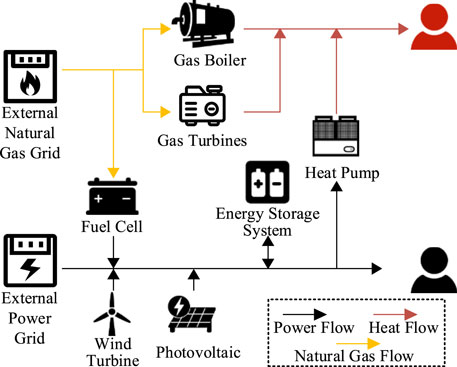
FIGURE 1. The structure of the micro energy network.

2.2 The equipment modelling in the multi-energy microgrid

2.2.1 Photovoltaic

The power generation of Photovoltaics (PV) is greatly affected by weather and environmental conditions, and mainly depends on solar irradiance and the ambient temperature. Based on research (Chen et al., 2021a), the power output of a PV array can be modeled as in (1):

$P^{\mathrm{P}\mathrm{V}}=P^{\mathrm{P}\mathrm{V},\mathrm{N}}\frac{G}{1000}\left[1+K^{\mathrm{p}}\left(T^{\mathrm{c}\mathrm{e}\mathrm{l}\mathrm{l}}-T^{\mathrm{c}\mathrm{e}\mathrm{l}\mathrm{l},\mathrm{S}\mathrm{T}\mathrm{C}}\right)\right](1)$

where $P^{\mathrm{P}\mathrm{V}}$ (kW) is the actual power output of the PV array; $G$ (W/m2) represents the solar irradiance; $P^{\mathrm{P}\mathrm{V},\mathrm{N}}$ (kW) is the maximum power output under the standard test condition; $K^{\mathrm{p}}$ (%/°C) is the temperature coefficient of power; $T^{\mathrm{c}\mathrm{e}\mathrm{l}\mathrm{l}}$ (°C) is the actual surface temperature of the PV array; and $T^{\mathrm{c}\mathrm{e}\mathrm{l}\mathrm{l},\mathrm{S}\mathrm{T}\mathrm{C}}$ (°C) is the PV surface temperature under the standard test condition, which is usually set as 25°C.

2.2.2 Wind turbine

Wind turbines (WT) capture the kinetic energy of the wind with their blades to make rotors rotate to create a magnetic field and finally generate electrical energy. Based on research (Chen et al., 2021a), a wind turbine’s power output is mainly related to the wind speed and can be modeled as in (2):

$P^{\mathrm{W}\mathrm{T}}=\left\{\begin{array}{l}0v\le v_{\mathrm{i}\mathrm{n}}\\ P^{\mathrm{W}\mathrm{T},\mathrm{N}}\frac{v^3-v_{\mathrm{i}\mathrm{n}}^3}{v_{\mathrm{N}}^3-v_{\mathrm{i}\mathrm{n}}^3}{v}_{\mathrm{i}\mathrm{n}}\le v\le v_{\mathrm{N}}\\ P^{\mathrm{W}\mathrm{T},\mathrm{N}}{v}_{\mathrm{N}}\le v\le v_{\mathrm{o}\mathrm{u}\mathrm{t}}\\ 0v\ge v_{\mathrm{o}\mathrm{u}\mathrm{t}}\end{array}\right.(2)$

where $P^{\mathrm{W}\mathrm{T}}$ (kW) and $P^{\mathrm{W}\mathrm{T},\mathrm{N}}$ (kW) are the actual output power and maximum power output of the WT; $v$ (m/s), $v_{\mathrm{i}\mathrm{n}}$ (m/s), $v_{\mathrm{N}}$ (m/s), and $v_{\mathrm{o}\mathrm{u}\mathrm{t}}$ (m/s) are respectively the actual wind speed, cut-in wind speed, rated wind speed, and cut-out wind speed.

2.2.3 Fuel cell

Fuel cells (FC) convert chemical energy in fuels such as natural gas, methane, and hydrogen into electricity (Lu et al., 2022). The power output of a fuel cell is modeled as in (3):

$P^{\mathrm{F}\mathrm{C}}={\eta }^{\mathrm{F}\mathrm{C}}{F}^{\mathrm{F}\mathrm{C}}{Q}_{\mathrm{L}\mathrm{H}\mathrm{V}}(3)$

where $P^{\mathrm{F}\mathrm{C}}$ (kW) is the output power of the FC; ${\eta }^{\mathrm{F}\mathrm{C}}$ represents the power generation efficiency; $F^{\mathrm{F}\mathrm{C}}$ (m³/s) is the natural gas inflow to the FC; and $Q_{\mathrm{L}\mathrm{H}\mathrm{V}}$ is the lower calorific value of natural gas, which is a constant parameter and set as 9.7 kW/m³.

2.2.4 Gas turbine

Gas turbines (GT) simultaneously generate electricity and heat by combusting gasoline, natural gas, hydrogen, or other fuels. The output of a gas turbine is modeled as in (4) considering natural gas as the fuel:

$\left\{\begin{array}{l}{P}^{\mathrm{G}\mathrm{T}}={\eta }^{\mathrm{G}\mathrm{T},\mathrm{e}}{F}^{\mathrm{G}\mathrm{T}}{Q}_{\mathrm{L}\mathrm{H}\mathrm{V}}\\ H^{\mathrm{G}\mathrm{T}}={\eta }^{\mathrm{G}\mathrm{T},\mathrm{h}}{F}^{\mathrm{G}\mathrm{T}}{Q}_{\mathrm{L}\mathrm{H}\mathrm{V}}\end{array}\right.(4)$

where $P^{\mathrm{G}\mathrm{T}}$ (kW) and $H^{\mathrm{G}\mathrm{T}}$ (kW) are the electrical power and thermal power output of the gas turbine; ${\eta }^{\mathrm{G}\mathrm{T},\mathrm{e}}$ and ${\eta }^{\mathrm{G}\mathrm{T},\mathrm{h}}$ respectively represent the power generation and heat production efficiencies; and $F^{\mathrm{G}\mathrm{T}}$ (m³/s) represents the natural gas inflow to the gas turbine.

2.2.5 Heat pump

Heat pumps (HP) driven by electrical motors that consume electricity can transfer the thermal energy from a low-temperature object to a high-temperature object without consuming additional primary energy. Referring to research (Huiling et al., 2021), the thermal power output of a head pump is modeled as in (5):

$H^{\mathrm{H}\mathrm{P}}={\eta }^{\mathrm{H}\mathrm{P}}{P}^{\mathrm{H}\mathrm{P}}(5)$

where $H^{\mathrm{H}\mathrm{P}}$ (kW) represents the thermal power output of the HP; ${\eta }^{\mathrm{H}\mathrm{P}}$ represents the heat production efficiency of the HP; $P^{\mathrm{H}\mathrm{P}}$ (kW) denotes the electrical power input of the HP.

2.2.6 Gas boiler

Gas boilers (GB) consume natural gas, liquefied gas, and others as the fuel to produce heat and are currently the most common heating equipment. Referring to research (Xuanyue et al., 2022), the thermal power output of a gas boiler can be modeled as in (6) with natural gas being the fuel:

$H^{\mathrm{G}\mathrm{B}}={\eta }^{\mathrm{G}\mathrm{B}}{F}^{\mathrm{G}\mathrm{B}}{Q}_{\mathrm{L}\mathrm{H}\mathrm{V}}(6)$

where $H^{\mathrm{G}\mathrm{B}}$ (kW) represents the thermal power output of the GB; ${\eta }^{\mathrm{G}\mathrm{B}}$ represents the heat production efficiency of the GB; $F^{\mathrm{G}\mathrm{B}}$ (kW) denotes the natural gas inflow to the GB.

2.2.7 Energy storage system

Energy Storage Systems (ESSs) can shift energy consumption and the model of a typical ESS is shown as in (7); (8) (Wu et al., 2023). Constraint (7) represents the energy evolution of the ESS. Constraint (8) guarantees that the stored energy of the ESS at the initial time interval is equal to that at the terminal time interval in the scheduling time horizon. In constraints (7) and (8), $E_t^{\mathrm{E}\mathrm{S}\mathrm{S}}$ (kWh) is the stored energy at time interval t. $P_t^{\mathrm{E}\mathrm{S}\mathrm{S},\mathrm{c}\mathrm{h}\mathrm{r}}$ (kW) and $P_t^{\mathrm{E}\mathrm{S}\mathrm{S},\mathrm{d}\mathrm{i}\mathrm{s}}$ (kW) are respectively the charging and discharging power during time interval t. ${\eta }^{\mathrm{E}\mathrm{S}\mathrm{S},\mathrm{c}\mathrm{h}\mathrm{r}}$ and ${\eta }^{\mathrm{E}\mathrm{S}\mathrm{S},\mathrm{d}\mathrm{i}\mathrm{s}}$ are corresponding charging and discharging efficiencies. ∆t represents the timespan of a time interval.

$E_t^{\mathrm{E}\mathrm{S}\mathrm{S}}=E_{t-1}^{\mathrm{E}\mathrm{S}\mathrm{S}}+\left({\eta }^{\mathrm{E}\mathrm{S}\mathrm{S},\mathrm{c}\mathrm{h}\mathrm{r}}{P}_t^{\mathrm{E}\mathrm{S}\mathrm{S},\mathrm{c}\mathrm{h}\mathrm{r}}-\frac{P_t^{\mathrm{E}\mathrm{S}\mathrm{S},\mathrm{d}\mathrm{i}\mathrm{s}}}{{\eta }^{\mathrm{E}\mathrm{S}\mathrm{S},\mathrm{d}\mathrm{i}\mathrm{s}}}\right)\Delta t(7)$

$E_0^{\mathrm{E}\mathrm{S}\mathrm{S}}=E_T^{\mathrm{E}\mathrm{S}\mathrm{S}}(8)$

3 Risk analysis and quantification of the cost of operational risk

3.1 Risk analysis

The inherent uncertainty of renewable energy resources makes the difficulties to accurately predict the outputs of the multi-energy microgrids, which may lead to deviations between the actual and scheduled power outputs during the operation phase. Consequently, the following risks may occur:

1) With a large installed capacity of renewable energy resources, wind and solar energy curtailment is prone to occur due to the excessive generation capacity.

2) With a low installed capacity of renewable energy resources, the multi-energy microgrid is prone to purchasing high-priced energy from external systems and even load shedding due to energy shortage.

3) With a certain installed capacity of renewable energy resources, if the planned capacity of multi-energy conversion equipment is insufficient, the system will lack operational flexibility, possibly causing wind and solar energy curtailment during load peaks and load shedding during load valleys.

4) If the planned capacity of multi-energy conversion equipment is redundant, although wind and solar energy curtailment and load shedding can be avoided with the excessive system operational flexibility, the investment cost will dramatically increase.

The above-mentioned risks that potentially occur during the operation phase of the multi-energy microgrid will be caused by an unappreciated capacity scheme of the equipment and the uncertainty of renewable energy. These risks occur with some probabilities. The probability of risk occurrence and the corresponding degree of loss jointly characterize the cost of operational risk that needs to be considered in the planning phase of the multi-energy microgrid. Therefore, CVaR is employed to quantify this cost of the operational risk.

3.2 CVaR based cost of operational risk quantification

CVaR is an improved variant of Value at Risk (VaR) (Roustai et al., 2018). VaR is widely used in the financial sector to express the maximum possible loss of an investment portfolio over a specified period of time in future at a certain confidence level. It can be expressed as in (9) and (10). In (9), X represents the decision variable in an investment portfolio and $\xi$ represents a random variable. For a given X, namely given the investment portfolio, $\mathrm{\Psi }\left(X,\cdot \right)$ represents the probability distribution function of the investment loss $f\left(X,\xi \right)$. Formula (10) defines VaR, where $\alpha$ represents a confidence level, which is usually set close to 1; $\alpha =0.9$, for example.

$\mathrm{\Psi }\left(X,y\right)=\mathrm{Pr}\left\{\xi |f\left(X,\xi \right)\le y\right\}(9)$

${\mathrm{V}\mathrm{a}\mathrm{R}}_{\alpha }=\min \left\{y|\mathrm{\Psi }\left(X,y\right)\ge \alpha \right\}(10)$

To make up for the shortcomings of VaR, such as high computational complexity and insufficient tail risk consideration, an improved variant of VaR, namely CVaR, was proposed (Wu et al., 2018). This index is defined as the loss that exceeds the mean value of VaR at a certain confidence level. Compared to VaR, CVaR can take the tail risk of the investment portfolio into consideration and effectively evaluate the loss degree when the worst case occurs. In general, CVaR is more comprehensive and conservative than VaR (Gao et al., 2015). CVaR can be expressed as in (11), where $p\left(\cdot \right)$ represents a probability density function.

${\mathrm{C}\mathrm{V}\mathrm{a}\mathrm{R}}_{\alpha }=E\left[f\left(X,\xi \right)|f\left(X,\xi \right)\ge {\mathrm{V}\mathrm{a}\mathrm{R}}_{\alpha }\right]=\frac{1}{1-\alpha }{\int }_{f\left(X,\xi \right)\ge {\mathrm{V}\mathrm{a}\mathrm{R}}_{\alpha }}f\left(X,\xi \right)p\left(\xi \right)\mathrm{d}\xi (11)$

Based on the definition of CVaR, the planning scheme and the corresponding cost are considered as “investment portfolio”, and the operating cost that contains penalties are seen as “possible losses”. Thereby CVaR can be adopted to describe the cost of the operational risk of a certain planning scheme, as shown in Figure 2. In terms of the formulation, in (11), the variable X represents the planning scheme of the equipment in the multi-energy microgrid; $\xi$ represents the output of wind and solar energy resources with randomness; and $f\left(X,{\xi }_s\right)$ represents the system operating cost with the planning scheme X and the wind and solar output scenario ${\xi }_s$.

FIGURE 2

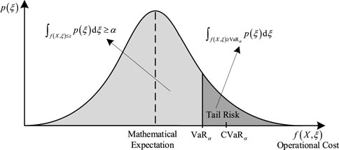
FIGURE 2. The risk of the operating cost.

Based on research (Lu et al., 2022), ${\mathrm{C}\mathrm{V}\mathrm{a}\mathrm{R}}_{\alpha }$ can be calculated by solving the purpose-built optimization problem (12). The optimal objective is ${\mathrm{C}\mathrm{V}\mathrm{a}\mathrm{R}}_{\alpha }$ and the solution to z is ${\mathrm{V}\mathrm{a}\mathrm{R}}_{\alpha }$.

$\min f\left(X,z\right)=z+\frac{1}{1-\alpha }{\displaystyle \sum }_{s=1}^S{p}_s{\left[f\left(X,{\xi }_s\right)-z\right]}^{+}(12)$

4 Multi-energy microgrid planning model considering the cost of operational risk

4.1 The objective of the planning model

The planning model built in this paper introduces WT and PV output as random variables, which belongs to Wait-and-See model (Li et al., 2016; Cao et al., 2021). To obtain several scenarios with probability, the scenario analysis method is utilized to discretize its probability distribution.

$\min C=C^{\mathrm{I}\mathrm{N}\mathrm{V}}+w\cdot C^{\mathrm{O}\mathrm{P}}+\left(1-w\right)\cdot C^{\mathrm{O}\mathrm{P},\mathrm{C}\mathrm{V}\mathrm{a}\mathrm{R}}(13)$

The objective of the multi-energy microgrid planning model, formulated as in (13), is to minimize the sum of the annual investment cost, the annual operating cost, and the cost of the operational risk. Among them, the cost of the operational risk is represented by CVaR. In (13), $C^{\mathrm{I}\mathrm{N}\mathrm{V}}$ is the equivalent annual investment cost of the multi-energy microgrid converted from the total investment cost. $C^{\mathrm{O}\mathrm{P}}$ is the expected value of the annual operating cost. $C^{\mathrm{O}\mathrm{P},\mathrm{C}\mathrm{V}\mathrm{a}\mathrm{R}}$ is the CVaR value of the annual operating cost, which characterizes the cost of the operational risk of a certain planning scheme. w is defined as the risk preference coefficient that indicates the decision maker’s preference of the risk. The higher the value of w is, the higher the acceptability of the risk is. Intuitively, a lower w indicates low acceptability of risk, which means the decision maker is more conservative.

4.1.1 Investment cost

Due to the differences in service life of different equipment, to take the influence of equipment service life into account in the investment cost, the net annual value method is adopted to convert the whole life cycle cost of the equipment to the equivalent annual investment cost. $C^{\mathrm{I}\mathrm{N}\mathrm{V}}$ is calculated as in (14):

$C^{\mathrm{I}\mathrm{N}\mathrm{V}}=\left[{\displaystyle \sum }_k^K{c}^k\cdot Ca{p}^k\cdot \frac{r\left(1+r\right)L^k}{\left(1+r\right)L^k-1}\right](14)$

where k denotes the equipment index; $c^k$ denotes the per kW investment cost of equipment k; $Ca{p}^k$ denotes the planned capacity of equipment k; r is the discount rate; and $L^k$ is the service life of equipment k.

4.1.2 Operating cost

The operating cost of the multi-energy microgrid, formulated as in (1), consists of energy purchase cost, maintenance cost, renewable energy curtailment penalty, and load shedding penalty. In (1), s is utilized to index the scenarios and d to index the typical days. $C_{s,d}^{\mathrm{B}\mathrm{U}\mathrm{Y}}$, $C_{s,d}^{\mathrm{O}\mathrm{M}}$, $C_{s,d}^{\mathrm{A}\mathrm{B}}$, $C_{s,d}^{\mathrm{C}\mathrm{U}\mathrm{R}}$ respectively represent energy purchase cost, maintenance cost, renewable energy curtailment penalty, load shedding penalty in scenario s of typical day d. $p\left(s\right)$ denotes as occurrence probability of scenario s; $N_d$ denotes the duration of typical day d. $F_{s,d,t}^{\mathrm{G}\mathrm{r}\mathrm{i}\mathrm{d}}$ and $P_{s,d,t}^{\mathrm{G}\mathrm{r}\mathrm{i}\mathrm{d}}$ are respectively the natural gas and electrical power purchased from the external nature gas grid and power grid at time interval t in scenario s of typical day d. $J^{\mathrm{G}}$ and $J_t^{\mathrm{E}}$ denote the natural gas price and the electricity price, in which the former is a constant and the latter is a time-of-use price. $R^k$ is the maintenance cost coefficient of equipment k. $P_{s,d,t}^k$ and $H_{s,d,t}^k$ are the power and thermal power outputs of equipment k at time interval t in scenario s of typical day d. $P_{s,d,t}^{\mathrm{E}\mathrm{S}\mathrm{S},\mathrm{c}\mathrm{h}\mathrm{r}}$ and $P_{s,d,t}^{\mathrm{E}\mathrm{S}\mathrm{S},\mathrm{d}\mathrm{i}\mathrm{s}}$ are the charging and discharging power of the ESS at time interval t in scenario s of typical day d. $P_{s,d,t}^{\mathrm{A}\mathrm{B}}$ and $H_{s,d,t}^{\mathrm{A}\mathrm{B}}$ respectively represent the electrical energy and heat curtailment at time interval t in scenario s of typical day d. ${\xi }^{\mathrm{E}}$, ${\xi }^{\mathrm{H}}$, ${\delta }^{\mathrm{E}}$, and ${\delta }^{\mathrm{H}}$ respectively denote the penalty prices of electrical energy curtailment, thermal energy curtailment, electrical load shedding, and thermal load shedding.

$\left\{\begin{array}{l}{C}^{\mathrm{O}\mathrm{P}}=\left[{\displaystyle \sum }_{s=1}^{S}p\left(s\right)\cdot C_s^{\mathrm{O}\mathrm{P}}\right]\\ C_s^{\mathrm{O}\mathrm{P}}={\displaystyle \sum }_{d=1}^D{N}_d\cdot \left(C_{s,d}^{\mathrm{B}\mathrm{U}\mathrm{Y}}+C_{s,d}^{\mathrm{O}\mathrm{M}}+C_{s,d}^{\mathrm{A}\mathrm{B}}+C_{s,d}^{\mathrm{C}\mathrm{U}\mathrm{R}}\right)\\ C_{s,d}^{\mathrm{B}\mathrm{U}\mathrm{Y}}={\displaystyle \sum }_{t=1}^T\left(F_{s,d,t}^{\mathrm{G}\mathrm{r}\mathrm{i}\mathrm{d}}{J}^{\mathrm{G}}+P_{s,d,t}^{\mathrm{G}\mathrm{r}\mathrm{i}\mathrm{d}}{J}_t^{\mathrm{E}}\right)\\ C_{s,d}^{\mathrm{O}\mathrm{M}}={\displaystyle \sum }_{t=1}^T\begin{array}{l}\left[{\displaystyle \sum }_k^{\left\{\mathrm{W}\mathrm{T},\mathrm{P}\mathrm{V},\mathrm{G}\mathrm{T},\mathrm{F}\mathrm{C}\right\}}{R}^k{P}_{s,d,t}^k+{\displaystyle \sum }_k^{\left\{\mathrm{G}\mathrm{B},\mathrm{H}\mathrm{P}\right\}}{R}^k{H}_{s,d,t}^k\right.\\ \left.+{\displaystyle \sum }_k^{\left\{\mathrm{E}\mathrm{S}\mathrm{S}\right\}}{R}^k\left(P_{s,d,t}^{k,\mathrm{c}\mathrm{h}\mathrm{r}}+P_{s,d,t}^{k,\mathrm{d}\mathrm{i}\mathrm{s}}\right)\right]\end{array}\\ C_{s,d}^{\mathrm{A}\mathrm{B}}={\displaystyle \sum }_{t=1}^T\left({\xi }^{\mathrm{E}}{P}_{s,d,t}^{\mathrm{A}\mathrm{B}}+{\xi }^{\mathrm{H}}{H}_{s,d,t}^{\mathrm{A}\mathrm{B}}\right)\\ C_{s,d}^{\mathrm{C}\mathrm{U}\mathrm{R}}={\displaystyle \sum }_{t=1}^T\left({\delta }^{\mathrm{E}}{P}_{s,d,t}^{\mathrm{C}\mathrm{U}\mathrm{R}}+{\delta }^{\mathrm{H}}{H}_{s,d,t}^{\mathrm{C}\mathrm{U}\mathrm{R}}\right)\end{array}\right.(15)$

4.1.3 Cost of operational risk

The cost of the operational risk is denoted by $C^{\mathrm{O}\mathrm{P},\mathrm{C}\mathrm{V}\mathrm{a}\mathrm{R}}$ and can be calculated as in (16):

$C^{\mathrm{O}\mathrm{P},\mathrm{C}\mathrm{V}\mathrm{a}\mathrm{R}}=C^{\mathrm{O}\mathrm{P},\mathrm{V}\mathrm{a}\mathrm{R}}+\frac{1}{1-\alpha }\cdot {\displaystyle \sum }_{s=1}^S{\displaystyle \sum }_{d=1}^D{N}_d\cdot p\left(s\right)\cdot {\left[C_s^{\mathrm{O}\mathrm{P},\mathrm{C}\mathrm{V}\mathrm{a}\mathrm{R}}-C^{\mathrm{O}\mathrm{P},\mathrm{V}\mathrm{a}\mathrm{R}}\right]}^{+}(16)$

where $C^{\mathrm{O}\mathrm{P},\mathrm{V}\mathrm{a}\mathrm{R}}$ represents VaR value of the annual operating cost. $\alpha$ represents the confidence level. An auxiliary variable $\kappa$ is introduced to equivalently linearize (16) as (17) and (18):

$C^{\mathrm{O}\mathrm{P},\mathrm{C}\mathrm{V}\mathrm{a}\mathrm{R}}=C^{\mathrm{O}\mathrm{P},\mathrm{V}\mathrm{a}\mathrm{R}}+\frac{1}{1-\alpha }\cdot {\displaystyle \sum }_{s=1}^S{\displaystyle \sum }_{d=1}^D{N}_d\cdot p\left(s\right)\cdot \kappa (17)$

$\left\{\begin{array}{l}\kappa \ge C_s^{\mathrm{O}\mathrm{P},\mathrm{C}\mathrm{V}\mathrm{a}\mathrm{R}}-C^{\mathrm{O}\mathrm{P},\mathrm{V}\mathrm{a}\mathrm{R}}\\ \kappa \ge 0\end{array}\right.(18)$

4.2 Physical constraints

4.2.1 Capacity constraints of equipment

The upper bound of the plannable capacity of the equipment may be affected by the available space, the lower bound may be affected by the minimum installed capacity of the equipment. Therefore, the model should include the plannable capacity constraints of the equipment:

$u^{k,\mathrm{I}\mathrm{N}\mathrm{V}}Ca{p}^{k,\min }\le Ca{p}^k\le u^{k,\mathrm{I}\mathrm{N}\mathrm{V}}Ca{p}^{k,\max },k\in \left\{\mathrm{G}\mathrm{T},\mathrm{F}\mathrm{C},\mathrm{G}\mathrm{B},\mathrm{H}\mathrm{P},\mathrm{E}\mathrm{S}\mathrm{S}\right\}(19)$

$u^{k,\mathrm{I}\mathrm{N}\mathrm{V}}=\left\{\begin{array}{cc}0,& \mathrm{n}\mathrm{o}\mathrm{t}\mathrm{p}\mathrm{l}\mathrm{a}\mathrm{n}\mathrm{e}\mathrm{d}\\ 1,& \mathrm{p}\mathrm{l}\mathrm{a}\mathrm{n}\mathrm{e}\mathrm{d}\end{array}\right.(20)$

where $Ca{p}^{k,\min }$ and $Ca{p}^{k,\max }$ indicate the upper and the lower bounds of the plannable capacity of equipment k. Binary variable $u^{k,\mathrm{I}\mathrm{N}\mathrm{V}}$ indicates whether the equipment k is planned.

4.2.2 Power output constraints

All types of the energy generation equipment should meet their output upper and lower bounds:

$U_t^k\cdot {\chi }^{k,\min }Ca{p}^k\le P_{s,d,t}^k\le U_t^k\cdot {\chi }^{k,\max }Ca{p}^k,k\in \left\{\mathrm{G}\mathrm{T},\mathrm{F}\mathrm{C}\right\},\hspace{1em}\forall s,d,t(21)$

$U_t^k\cdot {\chi }^{k,\min }Ca{p}^k\le H_{s,d,t}^k\le U_t^k\cdot {\chi }^{k,\max }Ca{p}^k,k\in \left\{\mathrm{G}\mathrm{B},\mathrm{H}\mathrm{P}\right\},\hspace{1em}\forall s,d,t(22)$

where ${\chi }^{k,\max }$ and ${\chi }^{k,\min }$ are the ratios of the output upper and the lower bounds to the capacity of the equipment k. The indicators are set as 1 and 0.1 in this paper. Cap^k represents the capacity of equipment k. Binary variable $U_t^k$ represents the ON/OFF status of the equipment k at time interval t. $U_t^k$ = 1 means ON and $U_t^k$ = 0 means OFF.

4.2.3 Charging and discharging constraints of the ESS

The ESS should meet its power upper and lower bounds of charging and discharging and its energy storage capacity bounds:

${\chi }^{\mathrm{E}\mathrm{S}\mathrm{S},\min }Ca{p}^{\mathrm{E}\mathrm{S}\mathrm{S}}\le P_{s,d,t}^{\mathrm{E}\mathrm{S}\mathrm{S},\mathrm{c}\mathrm{h}\mathrm{r}}\le {\chi }^{\mathrm{E}\mathrm{S}\mathrm{S},\max }Ca{p}^{\mathrm{E}\mathrm{S}\mathrm{S}},\hspace{1em}\forall s,d,t(23)$

${\chi }^{\mathrm{E}\mathrm{S}\mathrm{S},\min }Ca{p}^{\mathrm{E}\mathrm{S}\mathrm{S}}\le P_{s,d,t}^{\mathrm{E}\mathrm{S}\mathrm{S},\mathrm{d}\mathrm{i}\mathrm{s}}\le {\chi }^{\mathrm{E}\mathrm{S}\mathrm{S},\max }Ca{p}^{\mathrm{E}\mathrm{S}\mathrm{S}},\hspace{1em}\forall s,d,t(24)$

$So{c}^{\min }Ca{p}^{\mathrm{E}\mathrm{S}\mathrm{S}}\le E_{s,d,t}^{\mathrm{E}\mathrm{S}\mathrm{S}}\le So{c}^{\max }Ca{p}^{\mathrm{E}\mathrm{S}\mathrm{S}},\hspace{1em}\forall s,d,t(25)$

where Cap^ESS represents the capacity of the ESS. ${\chi }^{\mathrm{E}\mathrm{S}\mathrm{S},\max }Ca{p}^{\mathrm{E}\mathrm{S}\mathrm{S}}$ and ${\chi }^{\mathrm{E}\mathrm{S}\mathrm{S},\min }Ca{p}^{\mathrm{E}\mathrm{S}\mathrm{S}}$ set the upper and the lower bounds of the charging and discharging power of the ESS. ${\chi }^{\mathrm{E}\mathrm{S}\mathrm{S},\max }$ and ${\chi }^{\mathrm{E}\mathrm{S}\mathrm{S},\min }$ are set to 0.5 and 0 in this paper. $So{c}^{\max }$ and $So{c}^{\min }$ denote the upper and the lower bounds of the state of charge of the ESS. They are respectively set as 90% and 10%. $E_{s,d,t}^{\mathrm{E}\mathrm{S}\mathrm{S}}$ represents the stored energy at time interval t in scenario s of typical day d.

4.2.4 Capacity limitations of interconnection transformer and pipelines

The multi-energy microgrid is connected to the external power grid and the natural gas grid through interconnection transformers and pipelines. The power injection and nature gas inflow from the external grids are limited by their capacities as in (26), where $P^{\mathrm{G}\mathrm{r}\mathrm{i}\mathrm{d},\max }$ is the upper bound of the power injection and $F^{\mathrm{G}\mathrm{r}\mathrm{i}\mathrm{d},\min }$ is the upper bound of the nature gas inflow.

$\left\{\begin{array}{l}0\le P_{s,d,t}^{\mathrm{G}\mathrm{r}\mathrm{i}\mathrm{d}}\le P^{\mathrm{G}\mathrm{r}\mathrm{i}\mathrm{d},\max }\\ 0\le F_{s,d,t}^{\mathrm{G}\mathrm{r}\mathrm{i}\mathrm{d}}\le F^{\mathrm{G}\mathrm{r}\mathrm{i}\mathrm{d},\max }\end{array}\right.,\hspace{1em}\forall s,d,t(26)$

4.2.5 Multi-energy flow and balance model

The multi-energy power flow and balance model adopted in this paper refers to research (Wu et al., 2023). This model includes an AC power flow model, a steady-state natural gas flow model, and a simplified thermal energy model that ignores the delay of the thermal transfer and the heat loss during the heat transfer process.

4.3 Solving methodology

The model building and solving process of the presented planning model is shown in Figure 3.

FIGURE 3

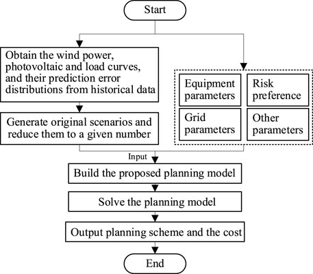
FIGURE 3. The model building and solving process.

Firstly, according to the historical wind speed, and solar irradiance, and load data, the wind power, photovoltaic and load curves, and their prediction error distributions are obtained. And then, on this basis, a large number of scenarios are generated leveraging Latin hypercube sampling method to simulate the uncertainty of wind and solar energy. These generated scenarios are then reduced with the crowding measure-based scenario reduction method to an appropriate number:

For any two scenes $X_i$ and $X_j$ ($\mathrm{i}\ne \mathrm{j}$), the distance between these scenes can be modeled:

$d_{ij}=\sqrt{{\displaystyle \sum }_{k=1}^n{\left(x_{ik}-x_{jk}\right)}^2}(27)$

The intensive distance of $X_i$ can be formulated as:

$c_i=\frac{d_{ia}+d_{ib}}{2}(28)$

where $a$ and $b$ are the numbers of the scenes most close to the scene $X_i$, $d_{ia}$ and $d_{ib}$ are the corresponding distances.

The importance of scene $i$ is defined as:

$I_i=c_i{p}_i(29)$

where $p_i$ is the probability of the appearance of scene $i$.

Then, calculate all $I$ s, and eliminate the scene with the minimum $I$. Update the probability of $X_a$ and $X_b$ by (30):

$\left\{\begin{array}{c}{p}_a=p_a+\frac{d_{ib}}{d_{ia}+d_{ib}}{p}_i\\ p_b=p_b+\frac{d_{ia}}{d_{ib}+d_{ia}}{p}_i\end{array}\right.(30)$

Repeat the above process until the number of remaining scenes meet the requirements.

Afterwards, the data and settings including the risk preference coefficient of the model, the equipment parameters, and the grid parameters are input into the proposed model. After the solution of the model, the planning scheme can be obtained.

5 Case study

5.1 The case setup

The presented model is verified using the multi-energy microgrid which is shown in Figure 4. Plannable devices include ESS, GT, GB, FC, HP, WT and PV in the multi-energy microgrid. Considering that the capacity of the equipment is usually an integer, the change step of the plannable equipment’s capacity is set as 10 kW. The parameters of the multi-energy microgrid are set as follows:

1) The capacities of the interconnection transformer and the natural gas pipeline of the multi-energy microgrid, namely $P^{\mathrm{G}\mathrm{r}\mathrm{i}\mathrm{d},\max }$ and $F^{\mathrm{G}\mathrm{r}\mathrm{i}\mathrm{d},\max }$, are respectively set as 800 kW and is 300 m³.

2) The natural gas price is set as $0.357/m³, and the electricity time-of-use prices are shown in Table 1. The penalty prices for the electrical energy curtailment, the thermal energy curtailment, the electrical load and the thermal load shedding (${\xi }^{\mathrm{E}}$; ${\xi }^{\mathrm{H}}$; ${\delta }^{\mathrm{E}}$,; ${\delta }^{\mathrm{H}}$) are respectively $0.296/kWh, $0.296/kWh, $0.267/kWh and $0.267/kWh.

3) Three typical days respectively representing winter, summer, spring and autumn and lasting 90 days, 90 days and 180 days in a year are generated. The load curves, wind energy output curves, and solar energy output curves of three typical days are shown in Figure 4. The peak of the electrical load is 2000 kW and the peak of the thermal load is 1600 kW.

FIGURE 4

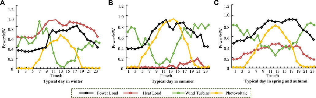
FIGURE 4. Load curves, wind energy and solar energy output curves of the three typical days. (A) Typical day in winter. (B) Typical day in summer. (C) Typical day in spring and autumn.

TABLE 1

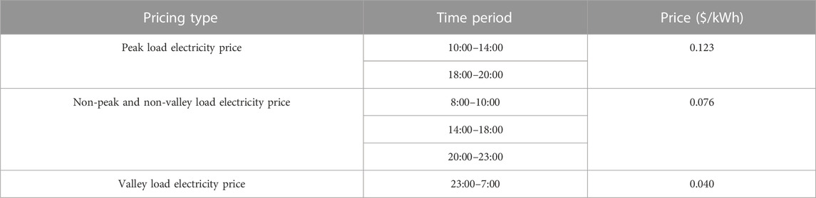
TABLE 1. Time-of-use electricity prices.

4) The relevant parameters of the equipment are shown in Table 2 and Table 3.

TABLE 2

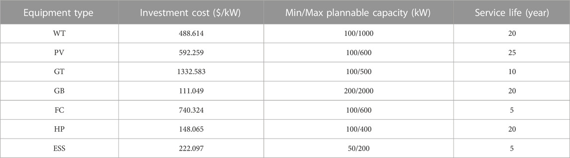
TABLE 2. Planning parameters of the equipment.

TABLE 3

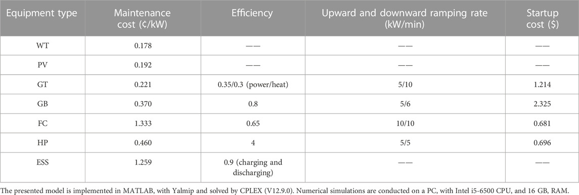
TABLE 3. Operating parameters of the equipment.

5.2 Scenario generation and reduction

According to the forecasted wind energy and solar energy curves, by setting the standard deviation as 20% of the output, 500 original scenarios are generated, and each of them has a probability of 0.002, as shown in Figure 5.

FIGURE 5

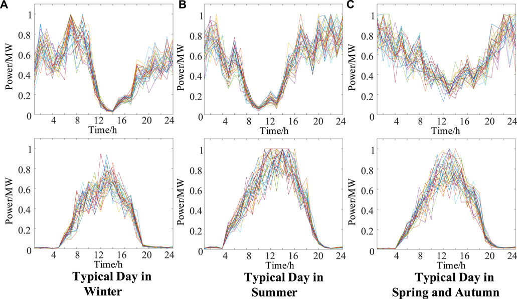
FIGURE 5. 500 original scenarios. (A) Typical day in winter. (B) Typical day in summer. (C) Typical day in spring and autumn.

Using the crowding measure-based scenario reduction method, the 500 original scenarios are reduced to 30 scenarios as shown in Figure 6, and the probability of each scenario is shown in Table 4.

FIGURE 6

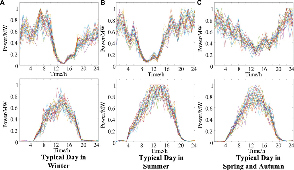
FIGURE 6. 30 scenarios after reduction. (A) Typical day in winter. (B) Typical day in summer. (C) Typical day in spring and autumn.

TABLE 4

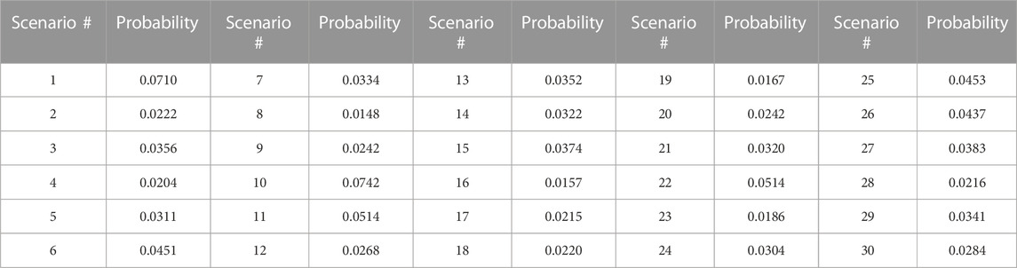
TABLE 4. Probabilities of 30 scenarios.

5.3 Planning result analysis

5.3.1 Planning scheme analysis

To validate the presented model, the risk preference coefficients are set as 0.01 (for approximately simulating the deterministic situation), 0.5, and 0.9 respectively, and the confidence level is set to 0.9. The corresponding planning schemes are shown in Table 5.

TABLE 5

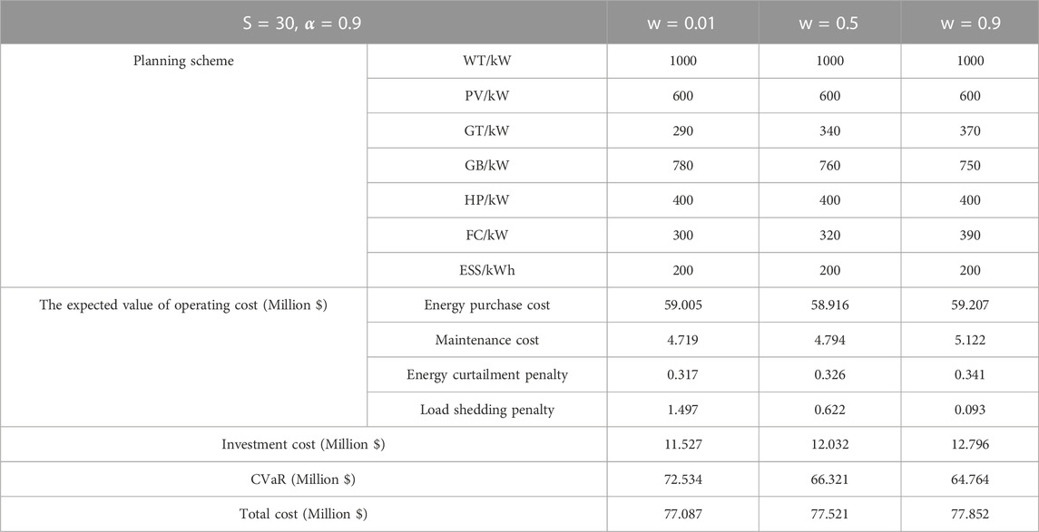
TABLE 5. Planning schemes with different risk preference coefficients.

It can be seen from Table 5 that:

1) Under various settings, the planned capacities of WT, PV, HP, and ESS all reach the upper bounds of their plannable capacities. This is because these types of equipment are more economical. For WT and PV, their service lives are long and the costs of generating green energy are low. For HP, its service life is also long, and its electro-thermal conversion efficiency is as high as 4, so it is also economical. For ESS, although its service life is relatively short, working together with WT and PV, it can play to the advantage of low generation cost of renewable energy effectively through peak-valley arbitrage.

2) With the increase of the capacity of GT, the capacity of GB decreases. This is because GT is capable of cogeneration. The increased capacity of GT can supply not only part of the electrical load, but also part of the thermal load. Therefore, considering the overall economic efficiency, the capacity of GB that provides heat only is reduced accordingly.

3) With the increasing risk preference coefficient, the capacities of GT and FC are gradually increasing as well. Moreover, the load shedding capacity goes down. Compared to w = 0.1, for w = 0.5 and w = 0.9, although the investment costs respectively increase by $5049.009 and $12689.153, the CVaR values decrease by $62127.987 and $77704.403, and the load shedding costs are reduced by 58.46% and 93.77%. It can be seen from Table 5 that the load shedding cost is an important parameter affecting CVaR, which demonstrates that the load shedding is the main factor of the operational risk. Therefore, to avoid the risk of load shedding caused by the uncertainty of wind and solar energies during the operation phase, the value of w should be set as relatively large, which indicates that the decision maker will be more inclined to plan more energy resources to deal with the uncertainty of renewable energy.

Figure 7 shows that with the increase of risk preference coefficient, the load shedding will gradually decrease, approaching zero.

4) The above results and analysis verify the effectiveness of the presented model and show that the model can reduce the risk of the system operation through adjusting the planning scheme.

FIGURE 7

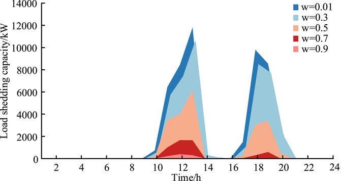
FIGURE 7. The distribution of operating cost.

To further validate the presented planning model and analyze the rationality of the planning results, based on the planning scheme of w = 0.5, the operating costs under the 500 original scenarios are calculated and plot the results as in Figure 8A. To make it clear, the expected value of operating cost, VaR values, and CVaR values are shown in Figure 8B.

FIGURE 8

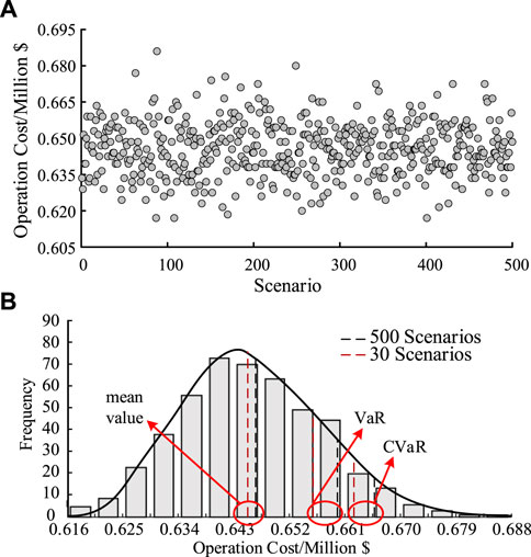
FIGURE 8. The distribution of operating cost. (A) The scatter chart of operating cost, (B) The chart of operating cost distribution, VaR and CVaR.

Table 6 shows the comparison of the results before and after scenario reduction. It can be seen that with 30 scenarios, the expected value of operating cost, VaR, CVaR and the total cost all merely slightly deviate from the results with 500 scenarios. In other words, the scenarios after reduction are still representative. In terms of computational efficiency, using merely 30 scenarios can significantly reduce the computational intensity.

TABLE 6

TABLE 6. Comparison of the results before and after scenario reduction.

5.3.2 Analysis of the impact of renewable energy forecast error on planning results

To discuss the impact of renewable energy forecast error on the planning results, the forecast error is set to increase from 0.1 times the standard deviation to 0.5 times the standard deviation in steps of 0.1. Under the condition of w = 0.5, the results calculated are shown in the following table:

It can be seen from Table 7 that with the rise of prediction error, the maintenance cost, renewable energy curtailment penalty, load shedding penalty, investment cost, cost of operational risk, and total cost, in the planning results increase. The reason is that after the prediction error increases, the volatilities of WT and PV output mount up, and more extreme scenarios appear. Correspondingly, the cost of operational risk, renewable energy curtailment penalty, and load shedding penalty goes up. Consequently, to avoid frequent load shedding and power curtailment, the system supplements the capacity of the equipment. Thus, the investment cost and maintenance cost increase.

TABLE 7

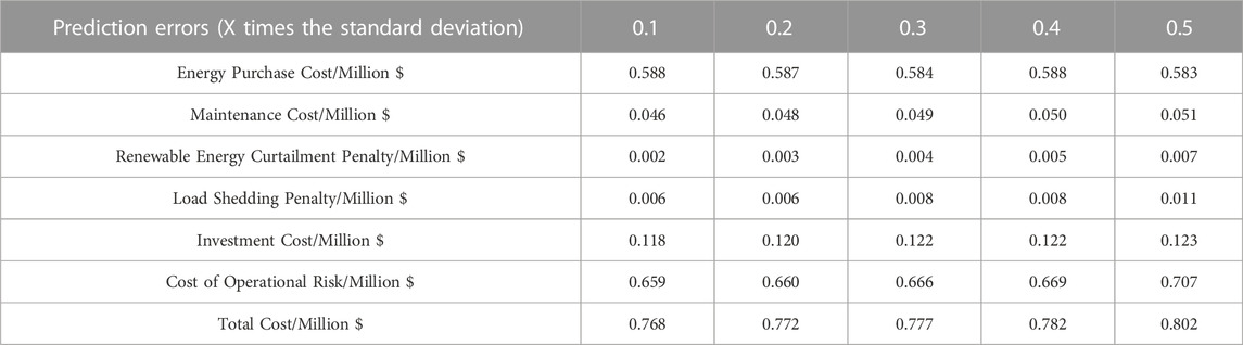
TABLE 7. The cost under the different renewable energy forecast errors.

5.3.3 The study of confidence level

To study the impact of the confidence level on the planning results, $\alpha$ is set as 0.8, 0.85, 0.9, 0.95, and 0.99. In these cases, w = 0.5 and the 30 scenarios are employed. The planning results, including the total costs, VaR values, and CVaR values, are compared in Figure 9.

FIGURE 9

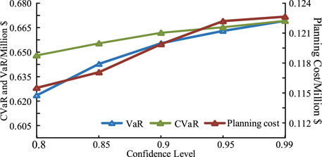
FIGURE 9. Total costs, VaR values, and CVaR values with different confidence levels.

As can be seen from Figure 9, with the increasing confidence level, the values of VaR and CVaR are getting larger, indicating that the risk faced by the multi-energy microgrid during the operation phase is gradually increasing. In addition, the difference between CVaR and VaR gradually shrinks as the confidence level increases until they finally become equal. This is because the wind and solar energy outputs follow normal distribution to some extent. From Figure 8, it can be seen that the operating cost corresponding to each output scenario is approximately normally distributed. The increase of $\alpha$ makes the operational risk gradually approach the tail of the normal distribution. As the probability density of the tail of the normal distribution is small, CVaR and VaR values are getting closer.

5.3.4 Analysis of planning schemes with different combinations of plannable equipment

To study the planning schemes with different combinations of the plannable equipment, three cases are set:

Case 1. WT, PV, GT, GB, FC, HP, ESS are the equipment to be planned.

Case 2. WT, PV, GT, GB, FC, HP are the equipment to be planned.

Case 3. WT, PV, GB, FC are the equipment to be planned.Table 8 shows the Comparing the planning schemes and costs in different cases. In Case 1 and Case 2, it can be seen that with the ESS being planned in Case 1, the energy purchase cost, the load shedding penalty, the energy curtailment penalty, and CVaR all decrease significantly. This is mainly because the ESS can store the electrical energy generated by the renewable energy resources during the low electricity price period and discharge during the peak load period with high electricity prices. Through peak load shifting, the ESS can effectively relieve energy supply pressure, which reduces the total operating cost and helps to deal with the uncertainty.Comparing Case 2 and Case 3, it can be seen that the total cost of Case 3 is significantly higher than that of Case 2. This is because in Case 3, only the coupling on natural gas input between GB and FC exists, and the overall multi-energy complementation is weak. The dealing of the uncertainty of wind and solar energies merely relies on FC and the power injection from the external power grid. This shows that the multi-energy microgrid lacks operational flexibility. The GT planned in Case 2 can build electricity-gas-thermal coupling, and the HP can build electricity-thermal coupling. Compared to Case 3, the multi-energy complementation between multiple energy is stronger, which ultimately reduces the operating cost considerably.

TABLE 8

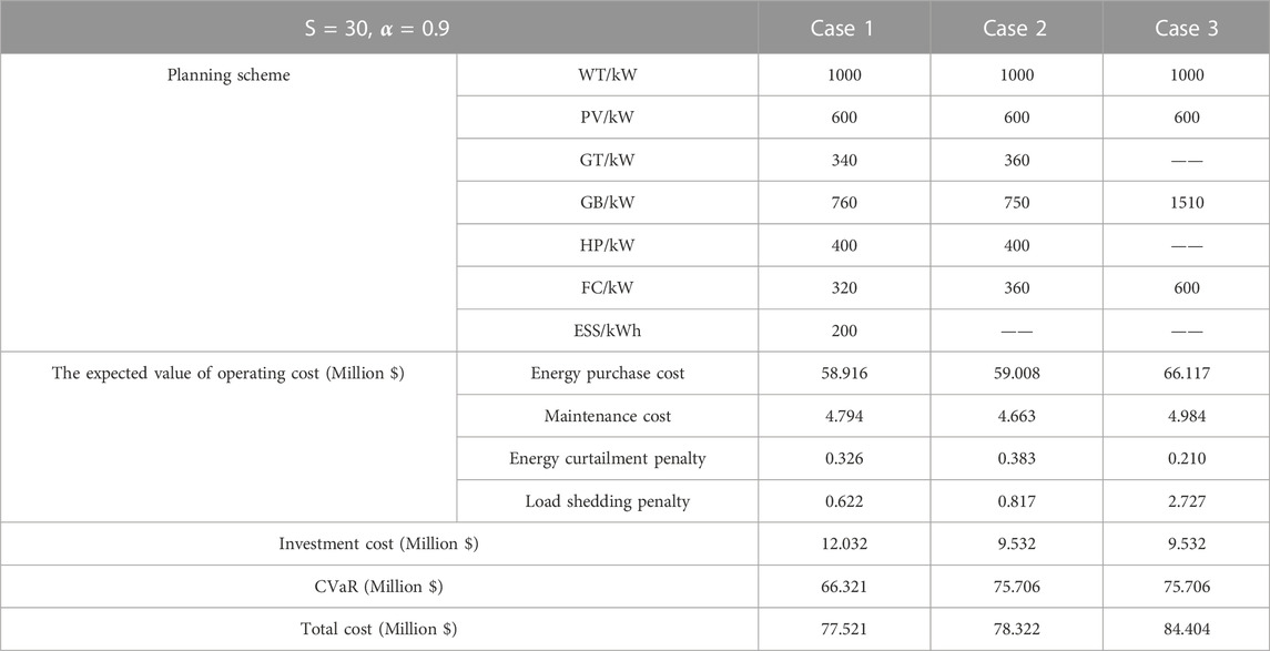
TABLE 8. Planning schemes with different combinations of plannable equipment.

5 Conclusion

Focusing on the risk brought by the uncertainty of wind and solar energy in multi-energy microgrids, this paper introduces CVaR to quantify the cost of the operational risk. On this basis, a multi-energy microgrid planning model that minimizes the investment cost, the operating cost, and the cost of the operational risk, while considering the physical limitations of the equipment, is presented. The following conclusions can be drawn through the case study:

1) The presented model can reduce the risk of the excessive operating costs by appropriately increasing the planned capacities of the energy resources and effectively balance the investment costs and the cost of the operational risk.

2) Decision makers can obtain either conservative or aggressive planning schemes through adjusting the risk preference coefficient w.

3) Energy storage systems in the multi-energy microgrid and a higher degree of multi-energy complementation can effectively mitigate the impact of the uncertainties from wind and solar energies and significantly reduce the operating cost and the cost of the operational risk.

The future research of this paper can be considered from the following two aspects:

1) The consideration of load side uncertainty can be added.

2) The thermal network in the multi-energy microgrid has heat storage performance. The constraints of the multi-energy network can be added to the model.

Data availability statement

The original contributions presented in the study are included in the article/supplementary material, further inquiries can be directed to the corresponding author.

Author contributions

RA and YY conceived the idea of the study and established the basic models, who innovatively considered CVaR in the configuration process of multi-energy microgrids. XL and RT designed the case studies and keenly analyzed the data and the results. JY and ZH specifically wrote the initial draft and then completed the substantive translation. All authors participated in the critical review and revision.

Funding

The authors would like to highly appreciate the support provided by the science and technology project of China Southern Power Grid Co., Ltd. (Project no. 036100KK52210025 (GDKJXM20210921)). The funder was not involved in the study design, collection, analysis, interpretation of data, the writing of this article, or the decision to submit it for publication.

Acknowledgments

This is a short text to acknowledge the contributions of specific colleagues, institutions, or agencies that aided the efforts of the authors.

Conflict of interest

Authors RA, YY, XL, RT, JY, and ZH were employed by the Company Electric Power Research Institute of Guangdong Power Grid Co, Ltd.

Publisher’s note

All claims expressed in this article are solely those of the authors and do not necessarily represent those of their affiliated organizations, or those of the publisher, the editors and the reviewers. Any product that may be evaluated in this article, or claim that may be made by its manufacturer, is not guaranteed or endorsed by the publisher.

References

Alraddadi, M., Conejo, A. J., and Lima, R. M. (2021). Expansion planning for renewable integration in power system of regions with very high solar irradiation. J. Mod. Power Syst. Clean Energy 9 (03), 485–494. doi:10.35833/mpce.2019.000112

CrossRef Full Text | Google Scholar

Cao, X., Cao, T., Gao, F., and Guan, X. (2021). Risk-averse storage planning for improving RES hosting capacity under uncertain siting choices. IEEE Trans. Sustain. energy 12 (4), 1984–1995. doi:10.1109/tste.2021.3075615

CrossRef Full Text | Google Scholar

Chen, Q., Xie, R., Chen, Y., Liu, H., Zhang, S., Fei, W., et al. (2021). Power configuration scheme for battery energy storage systems considering the renewable energy penetration level. Front. Energy Res. 9, 340. 10.3389/fenrg.2021.718019.

CrossRef Full Text | Google Scholar

Chen, X., Yang, Y., Liu, Y., and Wu, L. (2021). Feature-driven economic improvement for network-constrained unit commitment: A closed-loop predict-and-optimize framework. 37, 3104–3118. doi:10.1109/TPWRS.2021.3128485

CrossRef Full Text | Google Scholar

Chen, Y., Xu, J., Wang, J., Lund, P. D., and Wang, D. (2022). Configuration optimization and selection of a photovoltaic-gas integrated energy system considering renewable energy penetration in power grid. Energy Convers. Manag. 254, 115260. doi:10.1016/j.enconman.2022.115260

CrossRef Full Text | Google Scholar

Chitalia, G., Pipattanasomporn, M., Garg, V., and Rahman, S. (2020). Robust short-term electrical load forecasting framework for commercial buildings using deep recurrent neural networks. Appl. Energy 278, 115410. doi:10.1016/j.apenergy.2020.115410

CrossRef Full Text | Google Scholar

Ding, X., Ma, H., Yan, Z., Jie, X., and Sun, J. (2022). Distributionally robust capacity configuration for energy storage in microgrid considering renewable utilization[J]. Front. Energy Res. 10, 896. 10.3389/fenrg.2022.923985.

CrossRef Full Text | Google Scholar

Gao, Y., Li, R., and Liang, H. (2015). Two step optimal dispatch based on multiple scenarios technique considering uncertainties of intermittent distributed generations and loads in the active distribution system. Proc. CSEE 35 (07), 1657–1665.

Google Scholar

Hasankhani, A., and Hakimi, S. M. (2021). Stochastic energy management of smart microgrid with intermittent renewable energy resources in electricity market. Energy 219, 119668. doi:10.1016/j.energy.2020.119668

CrossRef Full Text | Google Scholar

He, Y., Wu, H., Ding, M., Bi, R., and Hua, Y. (2023). Reduction method for multi-period time series scenarios of wind power. Electr. Power Syst. Res. 214, 108813. doi:10.1016/j.epsr.2022.108813

CrossRef Full Text | Google Scholar

Huiling, T., Jiekang, W., Lingmin, C., Zhijun, L., Fan, W., Kangxing, L., et al. (2021). A control optimization model for CVaR risk of distribution systems with PVs/DSs/EVs using Q-learning powered adaptive differential evolution algorithm. Int. J. Electr. Power & Energy Syst. 132, 107209. doi:10.1016/j.ijepes.2021.107209

CrossRef Full Text | Google Scholar

Kumar Barik, A., and Das, D. C. (2021). Integrated resource planning in sustainable energy-based distributed microgrids. Sustain. Energy Technol. Assessments 48, 101622. ISSN 2213-1388. doi:10.1016/j.seta.2021.101622

CrossRef Full Text | Google Scholar

Lei, Y., Wang, D., Jia, H., Li, J., Chen, J., Li, J., et al. (2021). Multi-stage stochastic planning of regional integrated energy system based on scenario tree path optimization under long-term multiple uncertainties. Appl. Energy 300, 117224. doi:10.1016/j.apenergy.2021.117224

CrossRef Full Text | Google Scholar

Li, J., Zhu, D., and Pan, Y. (2016). Comparative analysis of wait-and-see model for economic dispatch of wind power system. Electr. Power Constr. 37 (06), 62–69. (in Chinese). doi:10.3969/j.issn.1000-7229.2016.06.010

CrossRef Full Text | Google Scholar

Li, P., Wang, Z., Liu, H., Wang, J., Guo, T., and Yin, Y. (2021). Bi-level optimal configuration strategy of community integrated energy system with coordinated planning and operation. Energy 236, 121539. doi:10.1016/j.energy.2021.121539

CrossRef Full Text | Google Scholar

Li, Z., Wu, L., Xu, Y., Wang, L., and Yang, N. (2023). Distributed tri-layer risk-averse stochastic game approach for energy trading among multi-energy microgrids. Appl. Energy 331, 120282. doi:10.1016/j.apenergy.2022.120282

CrossRef Full Text | Google Scholar

Li, Z., Xu, Y., Feng, X., and Wu, Q. (2020). Optimal stochastic deployment of heterogeneous energy storage in a residential multienergy microgrid with demand-side management. IEEE Trans. Industrial Inf. 17 (2), 991–1004. doi:10.1109/tii.2020.2971227

CrossRef Full Text | Google Scholar

Li, Z., Wu, L., Xu, Y., Moazeni, S., and Tang, Z. (2021). Multi-stage real-time operation of a multi-energy microgrid with electrical and thermal energy storage assets: A data-driven mpc-adp approach. IEEE Trans. Smart Grid 13 (1), 213–226. doi:10.1109/tsg.2021.3119972

CrossRef Full Text | Google Scholar

Lin, C., Wu, W., Zhang, B., and Sun, Y. (2017). Decentralized solution for combined heat and power dispatch through benders decomposition. IEEE Trans. Sustain. energy 8 (4), 1361–1372. doi:10.1109/tste.2017.2681108

CrossRef Full Text | Google Scholar

Lin, J., Ma, J., Zhu, J., and Cui, Y. (2022). Short-term load forecasting based on LSTM networks considering attention mechanism. Int. J. Electr. Power & Energy Syst. 137, 107818. doi:10.1016/j.ijepes.2021.107818

CrossRef Full Text | Google Scholar

Liu, L., Liu, J., Ye, Y., Hui, L., Kun, C., Dong, L., et al. (2023). Ultra-short-term wind power forecasting based on deep Bayesian model with uncertainty. Renew. Energy. doi:10.1016/j.renene.2023.01.038

CrossRef Full Text | Google Scholar

Liu, W., Huang, Y., Li, Z., Yang, Y., and Yi, F. (2020). Optimal allocation for coupling device in an integrated energy system considering complex uncertainties of demand response. Energy 198, 117279. doi:10.1016/j.energy.2020.117279

CrossRef Full Text | Google Scholar

Lu, Y., Li, H., and Liu, Y. (2022). Optimal operation of electricity-gas-heat integrated energy system considering the risk of energy supply equipment failure. Power Syst. Prot. Control (in Chinese) 50 (09), 34–44.

Google Scholar

Mahzarnia, M., Moghaddam, M. P., Baboli, P. T., and Siano, P. (2020). A review of the measures to enhance power systems resilience. IEEE Systems Journal 14 (3), 4059–4070. doi:10.1109/jsyst.2020.2965993

CrossRef Full Text | Google Scholar

Roustai, M., Rayati, M., Sheikhi, A., and Ranjbar, A. (2018). A scenario-based optimization of Smart Energy Hub operation in a stochastic environment using conditional-value-at-risk. Sustainable cities and society 39, 309–316. doi:10.1016/j.scs.2018.01.045

CrossRef Full Text | Google Scholar

Shen, H., Zhang, H., Xu, Y., Chen, H., Zhu, Y., Zhang, Z., et al. (2022). Multi-objective capacity configuration optimization of an integrated energy system considering economy and environment with harvest heat. Energy Conversion and Management 269, 116116. doi:10.1016/j.enconman.2022.116116

CrossRef Full Text | Google Scholar

Wang, H., Xing, H., Luo, Y., and Zhang, W. (2023). Optimal scheduling of micro-energy grid with integrated demand response based on chance-constrained programming. International Journal of Electrical Power & Energy Systems 144, 108602. doi:10.1016/j.ijepes.2022.108602

CrossRef Full Text | Google Scholar

Wang, J., Du, W., and Yang, D. (2021). Integrated energy system planning based on life cycle and emergy theory. Frontiers in energy research, 414.

CrossRef Full Text | Google Scholar

Wang, L., Shi, Z., Dai, W., Zhu, L., Wang, X., Cong, H., et al. (2022). Two-stage stochastic planning for integrated energy systems accounting for carbon trading price uncertainty. International Journal of Electrical Power & Energy Systems 143, 108452. doi:10.1016/j.ijepes.2022.108452

CrossRef Full Text | Google Scholar

Wang, Y., Qiu, J., Tao, Y., and Zhao, J. (2020). Carbon-oriented operational planning in coupled electricity and emission trading markets. IEEE Transactions on Power Systems 35 (4), 3145–3157. doi:10.1109/tpwrs.2020.2966663

CrossRef Full Text | Google Scholar

Wu, J., Wu, Z., Wu, F., Tang, H., and Mao, X. (2018). CVaR risk-based optimization framework for renewable energy management in distribution systems with DGs and EVs. Energy 143, 323–336. doi:10.1016/j.energy.2017.10.083

CrossRef Full Text | Google Scholar

Wu, S., Li, H., Liu, Y., Lu, Y., and Wang, Z. (2023). A two-stage rolling optimization strategy for park-level integrated energy system considering multi-energy flexibility. International Journal of Electrical Power & Energy Systems 145, 108600. doi:10.1016/j.ijepes.2022.108600

CrossRef Full Text | Google Scholar

Xuan, A., Shen, X., Guo, Q., and Sun, H. (2021). A conditional value-at-risk based planning model for integrated energy system with energy storage and renewables. Applied Energy 294, 116971. doi:10.1016/j.apenergy.2021.116971

CrossRef Full Text | Google Scholar

Xuanyue, S., Wang, X., Wu, X., Wang, Y., Song, Z., Wang, B., et al. (2022). Peer-to-peer multi-energy distributed trading for interconnected microgrids: A general nash bargaining approach. International Journal of Electrical Power & Energy Systems 138, 107892. doi:10.1016/j.ijepes.2021.107892

CrossRef Full Text | Google Scholar

Yan, R., Wang, J., Lu, S., Ma, Z., Zhou, Y., Zhang, L., et al. (2021). Multi-objective two-stage adaptive robust planning method for an integrated energy system considering load uncertainty. Energy and Buildings 235, 110741. doi:10.1016/j.enbuild.2021.110741

CrossRef Full Text | Google Scholar

Zhang, Y., Le, J., Zheng, F., and Liu, K. (2019). Two-stage distributionally robust coordinated scheduling for gas-electricity integrated energy system considering wind power uncertainty and reserve capacity configuration. Renewable energy 135, 122–135. doi:10.1016/j.renene.2018.11.094

CrossRef Full Text | Google Scholar