 Peng Qiu1
 Chao Ding
- 1State Grid Zhejiang Electric Power Co., Ltd., Research Institute, Hangzhou, Zhejiang Province, China
- 2Hangzhou Mobius Tech Co., Ltd, Hangzhou, Zhejiang Province, China
With the large-scale wind power integration, power systems have to address not only the conventional power demand fluctuations but also the wind uncertainty. To improve the economical effectiveness, resilience, and environmental protection of power systems in the source-load uncertainty, a real-time low-carbon scheduling for the wind–thermal–hydro-storage integrated system is proposed. The power imbalance caused by the uncertainty is neutralized by the synergetic linear decision of multiple resources. To address the source-load uncertainty, a stochastic robust optimization is introduced, which establishes the system constraints by robust optimization for the resilience operation, while optimizing the expected operation cost in the empirical uncertainty distribution for economic efficiency. Moreover, a multi-point estimation is applied to formulate the expected operation cost precisely and quickly. By using the dual theory, the proposed real-time power scheduling is derived as a mixed integer bilinear constrained programming. A multi-step sequential convexified solution is developed to solve the complex scheduling problem, which linearizes the bilinear constraints with alternate optimization and relaxes the state variables of energy storages with an “estimation–correction” strategy. Finally, case studies show the superiority of the proposed scheduling method and convexified solution.
1 Introduction
Large-scale wind power integration is of great significance to energy conservation and emission reduction in power systems (Zhu et al., 2021; He et al., 2022). However, due to the fluctuating nature of wind power, the resilience operation of power systems faces the uncertainty challenge of both wind power and power demand. Real-time scheduling, as a part of multiple time-scale power scheduling, plays an important role in restoring the power balance and improving the system resilience (Surender et al., 2015; Zhou et al., 2018). Therefore, how to address the source-load uncertainty with the co-regulation of wind farms, thermal units, hydro units, energy storages, and other regulation resources in real-time scheduling to ensure the system security should be paid more attention.
At present, methods for the uncertainty problems mainly contain the stochastic optimization and robust optimization. The stochastic optimization (Liu et al., 2022; Li et al., 2023) formulates the source-load uncertainty with discrete scenarios. The method samples multiple scenarios according to the probability distribution of the source-load uncertainty and optimizes the expected operation cost formulated with these sampled scenarios (Li and Xu, 2019). However, it is difficult for these sampled scenarios to cover the whole uncertainty distribution, and hence, the system security cannot be guaranteed in some extreme scenarios. Moreover, the huge sample size and complex calculation also make it difficult for the stochastic optimization to meet the timeliness in real-time scheduling. By contrast, robust optimization methods are widely applied since they can cover the extreme scenarios of the source-load uncertainty. The widely applied robust optimization includes conventional robust optimization (CRO) (Zeng and Zhao, 2013), distributionally robust optimization (DRO) (Ding et al., 2022), and chance-constrained robust optimization (Qi et al., 2020; Li et al., 2022). CRO formulates the source-load uncertainty with the uncertainty set, i.e., the maximum possible space of uncertain scenarios. A two-stage robust unit commitment based on it is established (Bertsimas et al., 2013; Zhou et al., 2019), and the day-ahead scheduling is usually solved with the Benders duality method (Yang and Su, 2021) or column and constraint generation (C&CG) methods (Wang et al., 2022). Moreover, the regulation of energy storages is incorporated in the unit commitment, and a nested C&CG is developed to address the integer state variables of energy storages in the intraday regulation (Cobos et al., 2018). CRO only takes the boundary information of the uncertainty into account, while ignores the distribution information, and the methods usually lead to a conservative solution. In view of this, DRO formulates the source-load uncertainty with the ambiguous set (Wei et al., 2016; Zheng et al., 2021), i.e., the maximum possible space of uncertainty distribution, and optimizes the expected operation cost in the worst-case distributions. However, chance-constrained robust optimization (Qi et al., 2022) assumes that the constraints hold with a certain confidence level. The method improves the flexibility of the scheduling, while the system security is affected.
The aforementioned robust methods can be concluded as the adaptive optimization decision-based robust optimization. In the second stage of the scheduling (i.e., the adjustment stage), the adjustment of regulation resources adapting to the immediate source-load uncertainty is determined through an optimization procedure. However, the system power balance in the real-time scheduling is restored through the automatic generation control (AGC) system (Wu et al., 2017). According to the frequency deviation and tie-line power deviation of the regional power system, the AGC system obtains the power fluctuation from the deviation signals and allocates the adjusted power to regulation resources proportionally. The AGC system has a very high requirement for the decision time, and hence, the aforementioned adaptive optimization decision-based robust methods are inapplicable.
In addition to the adaptive optimization decision-based robust methods, the linear decision-based CRO and DRO (LCRO and LDRO) are also proposed. When the source-load uncertainty occurs, the regulation tasks are allocated to regulation resources, according to the affine factors, i.e., allocation coefficients. Therefore, the linear decision-based robust methods adapt to the real-time scheduling. The co-regulation of generation units and energy storages to wind uncertainty is realized based on LCRO (Jabr 2013). To improve the applicability of LCRO, the allowed interval of wind power is optimized in (Li X et al., 2015; Wang et al., 2019). The allowed upper bound is lower than the forecast upper bound, and hence the strategy makes LCRO applicable for systems with inadequate regulation capacity. In view of the conservativeness of LCRO, which optimizes the operation at the expected scenario, the LDRO-based scheduling model is developed for power systems (Xiong et al., 2017; Alismail et al., 2018). Considering that the worst-case distributions of the source-load uncertainty rarely happen, LDRO may lead to a non-optimal economical effectiveness in common distributions. To enhance the economic efficiency of robust methods in common distributions, a linear decision-based stochastic robust optimization (LSRO) is proposed in (Qu et al., 2020). The method establishes the system constraints using the robust optimization to guarantee the system resilience, while optimizes the operation cost in the empirical distribution of uncertainties for the economical effectiveness. The empirical distribution of uncertainties is the fitting of the existing historical scenarios, and it is closest to the real distribution of uncertainties. Therefore, LSRO shows an economical effectiveness in common distributions of uncertainties.
In view of the robustness and economical effectiveness of LSRO, this paper establishes the real-time scheduling for the wind–thermal–hydro-storage power system based on the method. This paper upgrades the traditional three-point estimation method to multi-point estimation and takes both wind uncertainty and power demand uncertainty into account. Moreover, the extreme scenario-based security constraints (Qu et al., 2020) tend to be conservative, and this study converts the system security constraints, containing the source-load uncertainty to deterministic bilinear constraints, according to dual theory. The proposed real-time power scheduling is derived as a mixed integer bilinear constraint programming, and a convexified solution is developed for the problem. The contributions are concluded as three points.
1) A real-time low-carbon scheduling for the wind–thermal–hydro-storage power system with the source-load uncertainty is established. The power imbalance of the system caused by the uncertainty is neutralized by the co-regulation of multiple resources. The source-load uncertainty is split into two uncertainty subsets to improve the flexibility of the linear decision. However, the carbon trading cost is introduced to realize a low-carbon system.
2) An improved LCRO is introduced to address the source-load uncertainty, which establishes the system constraints using the robust optimization for the resilience operation, while optimizes the expected operation cost in the empirical uncertainty distribution for the economical effectiveness. In addition to, a multi-point estimation is upgraded and applied to calculate the expected operation cost.
3) A multi-step sequential convexified solution is developed to solve the mixed integer bilinear constrained scheduling problem. The sign variables in the objective function are approximated with an initial convex model. The bilinear constraints in the problem are linearized with alternate optimization (AO). Also, the state variables of energy storages are addressed by an “estimation–correction” strategy such that the problem is derived as a convex quadratic programming.
2 Real-time power scheduling model with linear stochastic robust optimization
2.1 Source-load uncertainty set
The available wind power of wind farms and the real power demand equal the sum of forecast expectations and forecast errors as follows:
where
Considering that the regulation resources may be insufficient, a certain amount of wind curtailment is allowed to ensure the system security. Therefore, the system will determine an allowed upper bound of total wind fluctuations (
where PW m,t is the baseline power output of the wind farm m,
When considering the wind curtailment, the real wind fluctuation is smaller than the available wind fluctuation, and thus the system security constraints are only associated with the allowed wind fluctuation (i.e., real wind fluctuation). The uncertainty set of the allowed wind fluctuation is established as
where Ut is the total allowed wind fluctuation and
As for the power demand, load shedding is not allowed, and thus the uncertainty set for the forecast error of the power demand is formulated as
where Vt is the total power demand fluctuation.
Therefore, the source-load uncertainty set is a union set of the wind uncertainty set and power demand uncertainty set, which is given as: Ξt = ΞU t∪ΞV t.
2.2 Overall architecture of real-time scheduling
Real-time power scheduling optimizes the baseline power output of wind farms, thermal units, hydro units, and baseline charging power of energy storages, as well as the affine factors of non-wind regulation resources for the source-load uncertainty. The real-time power scheduling is usually performed in a rolling optimization way to determine the scheduling plan for the following 1 h period with 5 min resolution. When the wind power and power demand deviate from the baseline value, non-wind regulation resources including thermal units, hydro units, and energy storages co-regulate to restore the system power balance with the affine factors.
where
To sum up, the strategy for balancing the source-load uncertainty is presented as follows:
Power demand: Load shedding is not allowed, and power demands always trace the actual demands.
Wind farms: If the total available wind fluctuation is below the allowed upper bound
Non-wind resources: Thermal units, hydro units, and energy storages co-regulate as Eqs 5–7 to balance the source-load uncertainty.
2.3 System security constraints
1) Power balance:
2) Constraints of wind farms:
3) Constraints of thermal units:
where
4) Constraints of hydro units:
where
5) Constraints of energy storages:
where
6) Transmission limits of lines:
The maximum/minimum operation of wind farms, thermal units, hydro units, and energy storages occur at the extreme total source-load fluctuation, and hence their constraints are established using the extreme scenario method. As for transmission lines, their transmitted power is related to the power output of each wind farm and power demand of each node, which cannot be described with the total source-load fluctuation. Therefore, we formulate the transmission limits of lines as that concerning the source-load uncertainty as follows:
where
The transmission limits of lines can be described as the following compact form:
where A, B, C are constant vectors, d is a constant scalar, x is the decision variable vector, αj is the affine factor matrix, concerning the jth uncertainty subset, and π, λ, τ, and ϑ are dual variables, corresponding to constraints in the uncertainty subset Ξt,j.
By adopting the dual theory (Li et al., 2018), the constraint (29) with the source-load uncertainty is converted to a deterministic constraint as follows:
where e is a vector whose elements are all equal 1.
2.4 Optimized objective
The scheduling optimizes the baseline operation cost (i.e., the first stage) and the incremental cost expectation in the adjustment state (i.e., the second stage) as follows:
where Fbase is the baseline operation cost,
This paper introduces carbon trading (Wang et al., 2020a) to improve the environmental benefits of the resilient power system. The operation cost in the baseline state includes fuel costs of thermal units, system carbon trading costs, and penalty costs on the wind curtailment.
where Ci() is the quadratic fuel cost function of the thermal unit i, fc is the carbon trading costs of the system, and W() is the quadratic penalty cost function of the wind curtailment.
This study adopts the baseline method (Wang et al., 2020b; Guo et al., 2020) to calculate the carbon quota of the system, and the carbon trading cost of the system is formulated as follows:
where pc is the carbon trading price, ER and EQ are the baseline carbon emission and carbon quota of the system, respectively, βi,t is the carbon emission coefficient of the thermal unit i, anf ηc is the carbon quota for per unit of power generation.
The incremental cost expectation in the adjustment state includes the adjustment cost of thermal units and energy storages, incremental penalty costs on the wind curtailment, and incremental carbon trading costs. The traditional random sampling methods to formulate the output expectation usually requires a huge sampling scale to achieve an accurate estimation. In this paper, the multi-point estimation (Li Z et al., 2015) can uniformly cover the source-load uncertainty with a small scale of estimation points.
The multi-point estimation actually first determines the estimate vectors in the standard Gaussian distribution, then converts these estimate vectors to that of the source-load uncertainty, and finally calculates the output expectation (Li et al., 2008). The optimal estimate point number will be determined through sensitivity analysis in numerical simulations. The source-load uncertainty is assumed to be irrelevant in the time dimension, and thus only two uncertain variables are considered in the formulation of the incremental cost expectation, i.e. the available wind fluctuation and forecast error of the power demand. The incremental cost expectation in the adjustment state is formulated as
where r∈N is the index of uncertain variables, s∈M is the index of estimate points, ωs is the weight of the sth estimate point, (r, s) corresponds to the estimate vector concerning the rth uncertain variable and the sth estimate point, and zr,s is the estimate vector in the standard Gaussian distribution. In the estimate vector, the uncertain variable r equals the sth estimate point and other uncertain variables equal 0. Ψ is the cumulative distribution function of the standard Gaussian distribution. Ft−1 is the inverse of the cumulative distribution function of the source-load uncertainty.
Assume that the sign variable concerning the adopted affine factors in each estimate vector is σt,r,s. If σt,r,s = 1, the source-load power fluctuation is larger than 0, the system adopts the upward affine factors for the adjustment; else if σt,r,s = 0, the system adopts the downward affine factors for the adjustment. In each estimate vector, the incremental cost produced by thermal units and energy storages are calculated as
where Ut,r,s is the allowed wind fluctuation in the estimate vector (r, s), ρi,t, and pi,t are the incremental cost coefficient and regulation cost coefficient of the thermal unit i, respectively, and ρ− k, t ,and ρ+ k,t are the downward and upward incremental cost coefficient of the energy storage k. Since hydro units do not produce fuel costs and carbon emissions in the operation, their incremental cost coefficients equal 0. As for energy storages, since they also play a role of peak-load shifting and standby power generation during intraday operation, the stored power in storages after the scheduling shall not deviate too far from the required value. Therefore, the incremental cost coefficients are set as follows to reduce the adjustment of energy storages: ρ− k,t = -1.1 × maxi (ρi,t), ρ+ k,t = -0.9 × maxi (ρi,t).
To sum up, the incremental cost in each estimate vector is calculated as
where ρw is the penalty coefficient on the wind curtailment.
3 Solution methodology
The proposed scheduling model is a mixed integer bilinear constraint programming. The integer variables include the sign variables σt,r,s in each estimate vector concerning the incremental cost expectation and the charging/discharging state variables of energy storages. The bilinear constraints include Eq. 11 (15) (23) (30). Due to the timeliness required in the real-time scheduling, the integer variables and bilinear constraints shall be addressed, and such that the scheduling model can be converted to a convex quadratic programming.
3.1 Approximation for the sign variables
To determine the sign variables σt,r,s in each estimate vector concerning the incremental cost expectation, an approximated value for the allowed upper bound of wind fluctuation (
1) Objective of the initial model: The objective should be convex and can be close to the original objective (31). The objective of the initial model is
2) Constraints of the initial model: Reformulate the original bilinear constraints concerning the reserve constraints of non-wind regulation resources and transmission limits of lines with the extreme scenario method, while other security constraints remain unchanged. Therefore, the original bilinear constraints are converted to slightly conservative but convex linear constraints.
Therefore, the initial model does not contain the sign variables σt,r,s and bilinear constraints. Compare the available wind power in each estimate vector (
3.2 Linearization for bilinear constraints
This paper adopts the AO (Li et al., 2021) to address the bilinear constraints in the real-time scheduling, which fixes partial decision variables to optimize the rest of the decision variables in the bilinear constraints. The real-time scheduling with bilinear constraints can be described as the following compact form:
where Ai is a constant matrix, gi is a convex function concerning decision variables, y corresponds to the allowed upper bound of wind fluctuation (
Algorithm 1. AO to solve the bilinear problem.
1) Initialization: Solve the initial model as shown in Eqs 42–45 and obtain the initial value of the allowed upper bound of wind fluctuation (
2) Solve the sub-problem A: Fix y = yn and solve the below problem. The obtained x is marked as xn.
3) Solve the sub-problem B: Fix x = xn and solve the below problem. The obtained y is marked as yn+1, and the obtained objective is marked as Fn+1.
4) Convergence check: If the below condition is satisfied, stop the calculation, otherwise, update n = n+1 and return to step 2.
where the convergence gap ε is set to 10−6.
Note that AO is a sub-optimal method, whose optimization performance is associated with the initialization. To improve its optimization performance, the initial value of the allowed upper bound of wind fluctuation (
where
3.3 Approximation for state variables of energy storages
This paper adopts an “estimation–correction” strategy (Shi and Guo, 2022) to approximate the state variables of energy storages. The estimation stage relaxes the state variables of energy storages, and the correction stage directly determines the state variables according to the results obtained in the estimation stage.
Therefore, the scheduling problems in these two stages do not contain the state variables of energy storages. The relaxed model of energy storages in the estimation stage is formulated as
where
The state variables of energy storage are directly fixed in the correction stage. For the sake of convenience, the following takes the baseline scenario as an example, while the other two extreme scenarios can be disposed in a similar way.
where
In fact, there is generally little difference between the optimal state variables of energy storages in the estimation stage and the correction stage. On the one hand, the charging and discharging efficiency of energy storages are generally higher. In the real-time scheduling, only the energy storages with the rapid adjustment ability could be involved in the AGC system, such as the lithium storages, and the efficiency of lithium storages can reach about 90% at present (Shi and Guo, 2022). On the other hand, the current capacity of energy storages is generally small compared with the total power demand, and thus the relaxed model of energy storages in the estimation stage has slight influence on the optimized result.
The overall flowchart for the convexified solution is presented in Figure 1.
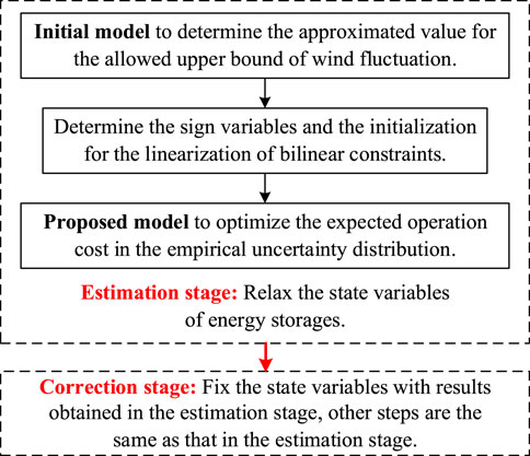
FIGURE 1. Overall flowchart for the convexified solution.
4 Numerical simulation
To illustrate the effectiveness of the proposed real-time low-carbon scheduling and solving method, numerical simulations are carried out on the IEEE 39-node power system (Zimmerman et al., 2011). The system has seven thermal units, one hydro unit, and two energy storages with 50MW capacity. Moreover, four wind farms are deployed. The scheduling cycle is from 6:00 pm to 7:00 pm with 5 min time resolution. The forecast expectation and forecast interval of wind power and power demand are presented in Figure 2 and Figure 3. Finally, 5,000 scenarios of the source-load uncertainty are sampled by Monte Carlo simulation (MCS) to verify the scheduling performance. The optimizations are solved with the CPLEX solver on a computer with Intel(R) Xeon(R) Silver 4216 CPU, 2.1GHz clock speed, and 16GB RAM.
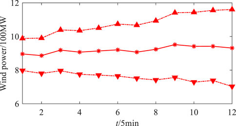
FIGURE 2. Forecast expectation and forecast interval of wind power.
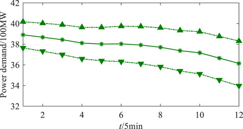
FIGURE 3. Forecast expectation and forecast interval of the power demand.
4.1 Effects of the allowed upper bound of wind fluctuation
In the proposed scheduling model, the allowed upper bound of wind fluctuation actually has two functions: 1) it reasonably determines the wind power accommodation and hence enhances the system flexibility, 2) when the system regulation capacity is insufficient, discard the excess wind power to ensure the system security. Figure 4 and Figure 5 present the allowed upper bounds (UB in the figures) of wind fluctuation in the system with sufficient and insufficient regulation capacity, where the maximum capacity of wind power accommodation is the obtained allowed upper bound of wind fluctuation when adding the wind penalty objective, i.e., the second line in Eq. 42, to the original objective. Moreover, in the system with insufficient regulation capacity, change the ramp rates of thermal units and hydro units as well as the maximum charging and discharging power of energy storages to 75% of the original.
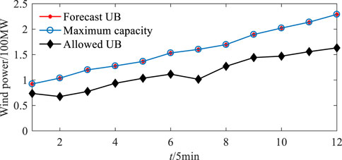
FIGURE 4. Allowed upper bound (UB) of wind fluctuation in the system with sufficient regulation capacity.
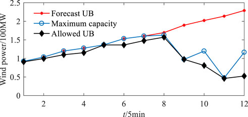
FIGURE 5. Allowed upper bound (UB) of wind fluctuation in the system with insufficient regulation capacity.
As shown in Figure 4, although the system with sufficient regulation capacity can completely accommodate wind power, partial wind power is still discarded. This is mainly because the wind fluctuation exceeding the allowed upper bound rarely appears, and hence these wind powers are discarded to improve the system flexibility. In addition to, as shown in Figure 5, the system with insufficient regulation capacity cannot completely accommodate wind power, and hence the allowed upper bound is below the forecast upper bound to ensure the system security. To further validate the effects of the allowed upper bound in improving the system flexibility, Table 1 compares the optimization results and MCS results with two wind power accommodation strategies. The maximum accommodation strategy is to absorb wind power as far as possible, while the flexible accommodation strategy is that in the proposed scheduling model. As shown in Table 1, although the allowed upper bound of wind fluctuation in the flexible strategy is obviously smaller than the maximum strategy, the discarded wind power is very slight. This is because the wind fluctuation exceeding the allowed upper bound rarely appears. Through the flexible accommodation strategy, the system operation cost is reduced, which validates the effects of allowed upper bound in improving the system flexibility.
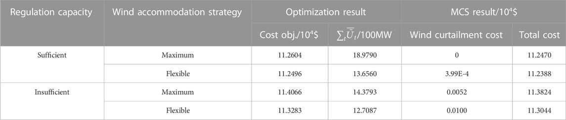
TABLE 1. Optimization and MCS results with different wind power accommodation strategies.
4.2 Baseline state and affine factors of regulation resources
Figure 6 presents the baseline outputs of thermal units and hydro units, and the baseline charging power of energy storages. Hydro units always operate at the maximum output since they do not produce fuel costs and carbon trading costs. Thermal units produce fuel costs and carbon trading costs, and hence, they arrange the outputs according to the cost-optimal principle. In the scheduling cycle of the testing case, the load peak is in the front period, while the load trough is in the latter period. Therefore, the energy storage is discharged according to the required state in the front period to realize the peak load shifting and reduce the operation cost.
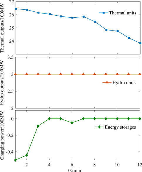
FIGURE 6. Baseline states of thermal units, hydro units, and energy storages.
Figure 7 and Figure 8 present the affine factors of thermal units, hydro units, and energy storages for the downward and upward source-load uncertainty, respectively. Affine factors of regulation resources are closely related to their incremental cost coefficients. When the source-load uncertainty fluctuates downward, the system operation cost is increased. The incremental cost coefficients of regulation resources satisfy
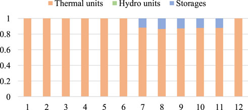
FIGURE 7. Affine factors for the downward source-load uncertainty.
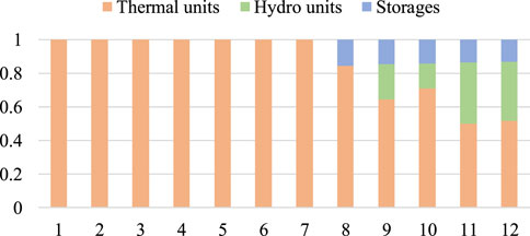
FIGURE 8. Affine factors for the upward source-load uncertainty.
Moreover, the existing AGC system usually utilizes units for the regulation. Due to the rapid adjustment speed, energy storages can participate in the AGC system to regulate the source-load uncertainty. To validate the effects of energy storages in the regulation, Table 2 compares the optimization results and MCS results without and with the regulation of energy storages.

TABLE 2. Optimization and MCS results without and with the regulation of energy storages.
4.3 Comparison of different robust methods
In order to further verify the economic efficiency of the LSRO, we compare it with LCRO and LDRO. The robust methods all optimize the allowed upper bound of wind fluctuation. The difference of these three robust methods is that, LSRO optimizes the expected cost under the empirical distribution of the source-load uncertainty, LCRO minimizes the baseline cost and maximizes the allowed upper bound of wind fluctuation, and LDRO minimizes the expected cost under the worst-case distributions of the source-load uncertainty. As shown in Table 3, LCRO minimizing the baseline cost ignores the impact of the adjustment process on the operation cost, and hence its adjustment is uneconomical. LDRO minimizes the expected cost under the worst-case distributions, however, the worst-case distributions rarely appear, and hence LDRO actually sacrifices the economic efficiency in general distributions for robustness in worst cases. The empirical distribution is the fitting of the historical scenarios, which is closest to the real distribution of the source-load uncertainty, and hence LSRO shows the best economic efficiency.

TABLE 3. Comparison of robust methods in the IEEE 39-node system.
4.4 Impacts of estimate point numbers
This paper upgrades the traditional three-point estimation to multi-point estimation. The estimate point numbers are set at 3, 5 and 7, respectively and results with different numbers are compared. Figure 9 shows the allowed upper bound of wind fluctuation obtained by multi-point estimation with different point numbers. The maximum cumulative distribution function covered by estimate points in three-point estimation, five-point estimation, and seven-point estimation are 0.9584, 0.9979, and 0.9999, respectively. The distribution of uncertain variables covered by three-point estimation is limited, while the uncertainty distribution covered by five-point estimation and seven-point estimation is large enough. Therefore, the allowed upper bound of wind fluctuation obtained by three-point estimation is much smaller compared to that obtained by five-point estimation and seven-point estimation. In addition, Table 4 compares the results of optimization and MCS with different point numbers, and it can be seen that there is little difference between the results. Considering that the seven-point estimation can cover the maximum distribution of uncertain variables, and the approximate degree of the expected value evaluation generally enhances with the increase in the point number (Li X et al., 2015), the estimate point number is set at 7 in this paper to ensure the robustness of the multi-point estimation method.
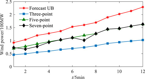
FIGURE 9. Allowed upper bound (UB) of wind fluctuation obtained with different point estimations.

TABLE 4. Optimization and MCS results with different point numbers.
4.5 Validation of solving methods
As indicated in subsection 3.2, AO is a sub-optimal method, whose optimization is related to initialization. This paper evenly sets the confidence level corresponding to initialization and updates the initial value of the allowed upper bound of wind fluctuation as Eq. 51. The results of optimization and MCS associated with the confidence level are presented in Table 5. Generally, the obtained allowed upper bound of wind fluctuation decreases with decrease in the confidence level. When the confidence level is high, the obtained allowed upper bound is large, and hence the wind curtailment is small. However, the system flexibility is affected due to excessive wind power accommodation, and thus the system operation cost increases. As the confidence level decreases, the obtained allowed upper bound decreases, the system flexibility improves, and the system operation cost is reduced. However, when the confidence level reaches 97.5%, the obtained allowed upper bound is too small, and hence the wind power accommodation is inadequate and the system operation cost gradually increases. Considering that the wind power prediction accuracy has a certain degree of error, the confidence level can be set at 99.7% to absorb wind power as far as possible without compromising the system’s flexibility.
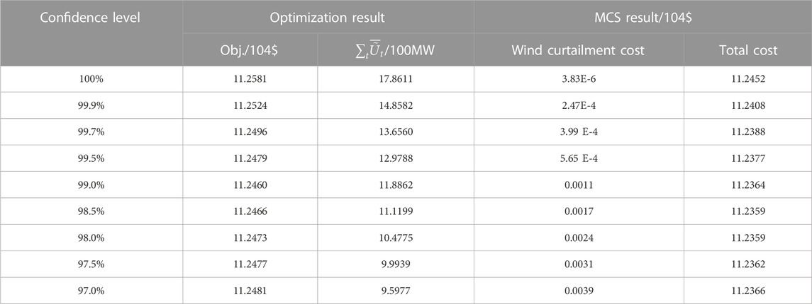
TABLE 5. Optimization and MCS results with different confidence levels.
In addition, the integer variables of charging/discharging state of energy storages are addressed with the estimation–correction strategy. Table 6 compares the optimization results with different strategies for the integer variables. The precise strategy takes the state variable of energy storage as variables in the optimization, and hence the scheduling problem is formulated as an iterative mixed integer quadratic constraint programming, which takes a long time to solve. The estimation stage relaxes the state variables, and the correction stage directly fixes the state variables as parameters, according to the results obtained in the estimation stage. Therefore, the scheduling problem is formulated as an iterative quadratic constraint programming with the estimation–correction strategy, and the computation time is short. On the other hand, the theoretically optimal objectives of these three strategies satisfy the following relations: Festimation < Fprecise < Fcorrection. Since the deviation between the optimization results of the estimation stage and the correction stage is small, it can be deduced that the estimation–correction strategy can find a good enough solution.
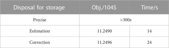
TABLE 6. Optimization results with different strategies for the state variables of energy storages.
4.6 Impacts of carbon trading price
Carbon trading cost is an important part of the proposed real-time low-carbon scheduling. To explore the influence of the carbon trading price on the scheduling, this subsection changes the carbon trading price from 0 to 60$/t and obtains the variation trend of the operation cost and carbon emission of the system relative to the carbon trading price. As indicated in Figure 10, carbon trading has little impact on the system operation when the carbon trading price is low, and thus the operation cost and carbon emissions change slightly. With the increase in the carbon trading price, the proportion of the carbon trading cost in the operation cost increases, the system gradually utilizes the low-carbon resources for power generation, and the carbon emission show a significant downward trend. When the carbon trading price rises to 26$/t, the system can make profits by the carbon trading mechanism, and the operation cost gradually decreases. When the carbon trading price rises to 40$/t, the carbon reduction space of the system becomes smaller, and the downward trend of carbon emissions slows down.
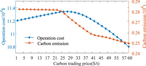
FIGURE 10. Variation trend in operation cost and carbon emissions relative to the carbon trading price.
5 Simulation in large-scale systems
5.1 Simulation results
To further verify the effectiveness of LSRO, supplementary simulations are performed in a large-scale IEEE 118-node power system. The system has seventeen thermal units, two hydro units, and four energy storages with 40MW capacity. Furthermore, six wind farms are deployed. As shown in Table 7, the results in the IEEE 118-node system are similar to those in the IEEE 39-node system. LCRO focuses on the baseline cost while ignores the influence of the adjustment on the operation cost, and the adjustment of the method is uneconomical. LDRO minimizes the expected cost under the worst-case distribution, in view of the extremely low probability of the worst-case distribution, and the method is not effective enough in common distributions. Compared to LCRO and LDRO, LSRO minimizes the expected cost under the empirical distribution of the source-load uncertainty. In view of that, the empirical distribution is closest to the real distribution of the source-load uncertainty, and LSRO shows the best economic efficiency.

TABLE 7. Comparison of robust methods in the IEEE 118-node system.
5.2 Further discussion on the robust method
In fact, the performance of LSRO is related to the accuracy of the empirical distribution of the source-load uncertainty. If the scale of historical scenarios is not huge enough or the adopted fitting method to determine the empirical distribution has a poor performance, the empirical distribution may deviate far from the real distribution. Therefore, the performance of the robust method in other distributions is affected in these cases. To improve the robustness of LSRO, our future work will combine the empirical distribution and worst-case distribution together in the robust method.
6 Conclusion
This paper proposes a real-time low-carbon scheduling for the wind–thermal–hydro-storage resilient power system based on the linear decision rule-based stochastic robust optimization. A multi-step alternate optimization-based convexified solution is formulated to solve the complex scheduling problem. The allowed upper bound of wind fluctuation provides the system with more flexibility. Monte Carlo simulation shows that very slight redundant wind power is sacrificed to significantly reduce the system operation cost. By the stochastic robust optimization, the regulation task to regulation sources is reasonably arranged according to the incremental cost coefficients of resources, and thus an economically effective adjustment is realized. The comparison of the adopted stochastic robust optimization with conventional robust optimization and distributionally robust optimization in two case studies validates the economic efficiency of the method. Numerical simulations indicate that the performance of alternate optimization is related to initialization, and the confidence level concerning the initialization can be reasonably set to absorb wind power as far as possible without compromising the system flexibility.
The empirical distribution of the source-load uncertainty may not be an accurate estimation of the real distribution, when the number of historical scenarios is inadequate or the fitting method is inaccurate. Our future work will combine the empirical distribution and worst-case distribution to improve the applicability of the linear decision-based robust method.
Data availability statement
The original contributions presented in the study are included in the article/Supplementary Material; further inquiries can be directed to the corresponding author.
Author contributions
PQ proposed the idea and conducted numerical simulations, YL provided the literature review, WZ and CD checked the paper for errors and modified the paper, and all authors discussed the results.
Funding
This work was supported by the State Grid Zhejiang Electric Power Co., Ltd., Science and Technology Project 5211DS200001.
Conflict of interest
Authors PQ, YL and CD were employed by State Grid Zhejiang Electric Power Co., LTD. Author WZ was employed by Hangzhou Mobius Tech Co., Ltd.
The authors declare that this study received funding from State Grid Zhejiang Electric Power Co., Ltd. The funder had the following involvement in the study: Providing the parameters of regulation resources and forecast information of the source-load uncertainty, as well as the simulation verification platform.
Publisher’s note
All claims expressed in this article are solely those of the authors and do not necessarily represent those of their affiliated organizations, or those of the publisher, the editors, and the reviewers. Any product that may be evaluated in this article, or claim that may be made by its manufacturer, is not guaranteed or endorsed by the publisher.
References
Alismail, F., Xiong, P., and Singh, C. (2018). Optimal wind farm allocation in multi-area power systems using distributionally robust optimization approach. IEEE Trans. Power Syst. 33 (1), 536–544. doi:10.1109/TPWRS.2017.2695002
Bertsimas, D., Litvinov, E., Sun, X., Zhao, J., and Zheng, T. (2013). Adaptive robust optimization for the security constrained unit commitment problem. IEEE Trans. Power Syst. 28 (1), 52–63. doi:10.1109/TPWRS.2012.2205021
Cobos, N. G., Arroyo, J. M., Alguacil, N., and Wang, J. (2018). Robust energy and reserve scheduling considering bulk energy storage units and wind uncertainty. IEEE Trans. Power Syst. 33 (5), 5206–5216. doi:10.1109/TPWRS.2018.2792140
Ding, X., Ma, H., Yan, Z., Xing, J., and Sun, J. (2022). Distributionally robust capacity configuration for energy storage in microgrid considering renewable utilization. Front. Energy Res. 10, 923985. doi:10.3389/fenrg.2022.923985
Guo, Z., Li, G., and Zhou, M. (2020). Fast and dynamic robust optimization of integrated electricity-gas system operation with carbon trading. Power Syst. Technol. 44 (4), 1220–1228. doi:10.13335/j.1000-3673.pst.2019.2313
He, R., Dong, P., Liu, M., Huang, S., and Li, J. (2022). A review of wind energy output simulation for new power system planning. Front. Energy Res. 10, 942450. doi:10.3389/fenrg.2022.942450
Jabr, R. A. (2013). Adjustable robust OPF with renewable energy sources. IEEE Trans. Power Syst. 28 (4), 4742–4751. doi:10.1109/TPWRS.2013.2275013
Li, H., Lv, Z., and Yuan, X. (2008). Nataf transformation based point estimate method. Chin. Sci. Bull. 53 (6), 2586–2592. doi:10.1007/s11434-008-0351-0
Li, X., Zhang, X., Wu, L., Lu, P., and Zhang, S. (2015). Transmission line over-load risk assessment for power systems with wind and load-power generation correlation. IEEE Trans. Smart Grid 6 (2), 1233–1242. doi:10.1109/TSG.2014.2387281
Li, Z., Wu, W., Zhang, B., and Wang, B. (2015). Adjustable robust real-time power dispatch with large-scale wind power integration. IEEE Trans. Sustain. Energy 6 (2), 357–368. doi:10.1109/TSTE.2014.2377752
Li, P., Yu, D., Yang, M., and Wang, J. (2018). Flexible look-ahead dispatch realized by robust optimization considering CVaR of wind power. IEEE Trans. Power Syst. 33 (5), 5330–5340. doi:10.1109/TPWRS.2018.2809431
Li, P., Yang, M., and Wu, Q. (2021). Confidence interval based distributionally robust real-time economic dispatch approach considering wind power accommodation risk. IEEE Trans. Sustain. Energy 12 (1), 58–69. doi:10.1109/TSTE.2020.2978634
Li, Z., Wu, L., Xu, Y., and Zheng, X. (2022). Stochastic-weighted robust optimization based bilayer operation of a multi-energy building microgrid considering practical thermal loads and battery degradation. IEEE Trans. Sustain. Energy 13 (2), 668–682. doi:10.1109/TSTE.2021.3126776
Li, Z., Wu, L., Xu, Y., Wang, L., and Yang, N. (2023). Distributed tri-layer risk-averse stochastic game approach for energy trading among multi-energy microgrids. Appl. Energy 331, 120282. doi:10.1016/j.apenergy.2022.120282
Li, Z., and Xu, Y. (2019). Temporally-coordinated optimal operation of a multi-energy microgrid under diverse uncertainties. Appl. Energy 240, 719–729. doi:10.1016/j.apenergy.2019.02.085
Liu, Y., Shen, Z., Tang, X., Lian, H., Li, J., and Gong, J. (2019). Worst-case conditional value-at-risk based bidding strategy for wind-hydro hybrid systems under probability distribution uncertainties. Appl. Energy 256, 113918. doi:10.1016/j.apenergy.2019.113918
Liu, H., Miao, Z., Wang, N., and Yang, Y. (2022). A two-layer optimization of design and operational management of a hybrid combined heat and power system. Front. Energy Res. 10, 959774. doi:10.3389/fenrg.2022.959774
Qi, F., Shahidehpour, M., Li, Z., Wen, F., and Shao, C. (2020). A chance-constrained decentralized operation of multi-area integrated electricity-natural gas systems with variable wind and solar energy. IEEE Trans. Sustain. Energy 11 (4), 2230–2240. doi:10.1109/TSTE.2019.2952495
Qu, K., Yu, T., Pan, Z., and Zhang, X. (2020). Point estimate-based stochastic robust dispatch for electricity-gas combined system under wind uncertainty using iterative convex optimization. Energy 211, 118986. doi:10.1016/j.energy.2020.118986
Shi, Y., and Guo, C. (2022). Flexibility reinforcement method for integrated electricity and heat system based on decentralized and coordinated multi-stage robust dispatching. Automation Electr. Power Syst. 46 (6), 10–19. doi:10.7500/AEPS20210311013
Surender, R. S., Bijwe, P. R., and Abhyankar, A. R. (2015). Real-time economic dispatch considering renewable power generation variability and uncertainty over scheduling period. IEEE Syst. J. 9 (4), 1440–1451. doi:10.1109/JSYST.2014.2325967
Wang, C., Wei, W., Wang, J., and Bi, T. (2019). Convex optimization based adjustable robust dispatch for integrated electric-gas systems considering gas delivery priority. Appl. Energy 239, 70–82. doi:10.1016/j.apenergy.2019.01.121
Wang, Y., Qiu, J., Tao, Y., and Zhao, J. (2020a). Carbon-oriented operational planning in coupled electricity and emission trading markets. IEEE Trans. Power Syst. 35 (4), 3145–3157. doi:10.1109/TPWRS.2020.2966663
Wang, Y., Qiu, J., Tao, Y., Zhang, X., and Wang, G. (2020b). Low-carbon oriented optimal energy dispatch in coupled natural gas and electricity systems. Appl. Energy 280, 115948. doi:10.1016/j.apenergy.2020.115948
Wang, Y., Qiu, J., and Tao, Y. (2022). Robust energy systems scheduling considering uncertainties and demand side emission impacts. Energy 239, 122317. doi:10.1016/j.energy.2021.122317
Wei, W., Liu, F., and Mei, S. (2016). Distributionally robust co-optimization of energy and reserve dispatch. IEEE Trans. Sustain. Energy 7 (1), 289–300. doi:10.1109/TSTE.2015.2494010
Wu, H., Krad, I., Florita, A., Hodge, B., Ibanez, E., Zhang, J., et al. (2017). Stochastic multi-timescale power system operations with variable wind Generation. IEEE Trans. Power Syst. 32 (5), 3325–3337. doi:10.1109/TPWRS.2016.2635684
Xiong, P., Jirutitijaroen, P., and Singh, C. (2017). A distributionally robust optimization model for unit commitment considering uncertain wind power generation. IEEE Trans. Power Syst. 32 (1), 39–49. doi:10.1109/TPWRS.2016.2544795
Yang, J., and Su, C. (2021). Robust optimization of microgrid based on renewable distributed power generation and load demand uncertainty. Energy 223, 120043. doi:10.1016/j.energy.2021.120043
Zeng, B., and Zhao, L. (2013). Solving two-stage robust optimization problems using a column-and-constraint generation method. Oper. Res. Lett. 41 (5), 457–461. doi:10.1016/j.orl.2013.05.003
Zheng, X., Qu, K., Lv, J., Li, Z., and Zeng, B. (2021). Addressing the conditional and correlated wind power forecast errors in unit commitment by distributionally robust optimization. IEEE Trans. Sustain. Energy 12 (2), 944–954. doi:10.1109/TSTE.2020.3026370
Zhou, A., Yang, M., Wang, Z., and Li, P. (2018). A linear solution method of generalized robust chance constrained real-time dispatch. IEEE Trans. Power Syst. 33 (6), 7313–7316. doi:10.1109/TPWRS.2018.2865184
Zhou, B., Ai, X., Fang, J., Yao, W., Zuo, W., Chen, Z., et al. (2019). Data-adaptive robust unit commitment in the hybrid AC/DC power system. Appl. Energy 254, 113784. doi:10.1016/j.apenergy.2019.113784
Zhu, Q., Wang, Y., Song, J., Jiang, L., and Li, Y. (2021). Coordinated frequency regulation of smart grid by demand side response and variable speed wind turbines. Front. Energy Res. 9, 754057. doi:10.3389/fenrg.2021.754057
Keywords: source-load uncertainty, real-time scheduling, stochastic robust optimization, dual theory, alternate optimization
Citation: Qiu P, Lu Y, Zhang W and Ding C (2023) Real-time low-carbon scheduling for the wind–thermal–hydro-storage resilient power system using linear stochastic robust optimization. Front. Energy Res. 11:1137305. doi: 10.3389/fenrg.2023.1137305
Received: 04 January 2023; Accepted: 18 January 2023;
Published: 23 January 2023.
Edited by:
Zhengmao Li, Nanyang Technological University, SingaporeReviewed by:
Yumin Zhang, Shandong University of Science and Technology, ChinaXiaodong Zheng, Southern Methodist University, United States
Zhengfa Zhang, The University of Manchester, United Kingdom
Yunqi Wang, Faculty of Information Technology, Monash University, Australia
Copyright © 2023 Qiu, Lu, Zhang and Ding. This is an open-access article distributed under the terms of the Creative Commons Attribution License (CC BY). The use, distribution or reproduction in other forums is permitted, provided the original author(s) and the copyright owner(s) are credited and that the original publication in this journal is cited, in accordance with accepted academic practice. No use, distribution or reproduction is permitted which does not comply with these terms.
*Correspondence: Chao Ding, Y2hhb19kaW5nMjAyM0AxNjMuY29t