State of energy estimation of the echelon-use lithium-ion battery based on Takagi–Sugeno fuzzy optimization

Owing to the degradation of an echelon-use lithium-ion battery (EULIB), the Ohmic internal resistance (OIR) and actual capacity (AE) have both changed greatly, and the state of energy (SOE) can more accurately represent the state of a EULIB than the state of charge (SOC) because of the working voltage. To improve the accuracy and adaptability of SOE estimation, in the paper, we study the energy state estimation of a EULIB. First, the four-order resistor–capacitance equivalent model of a EULIB is established, and an unscented transformation is introduced to further improve the estimation accuracy of the SOE. Second, a EULIB’s SOE is estimated based on adaptive unscented Kalman filter (AUKF), and the OIR and AE of a EULIB are estimated based on the AUKF. Third, a Takagi–Sugeno fuzzy model is introduced to optimize the OIR and AE of the EULIB, and the SOE estimation method is established based on an adaptive dual unscented Kalman filter (ADUKF). Through simulation experiments, verification, and comparison, energy decayed to 80%, 60%, and 40% of the rated energy, respectively, even with a large initial error; with the initial value of the SOE starting at 100%, 60%, or 20%, the estimated SOE can track the actual value. It can be seen that the method has a strong adaptive ability, and the estimation accuracy error is less than 1.0%, indicating that the algorithm has high accuracy. The method presented in this paper provides a new perspective for SOE estimation of EULIBs.

1 Introduction

An echelon-use lithium-ion battery (EULIB) refers to a power lithium battery with less than 80% capacity, which can be used as a backup power supply and on other occasions. Owing to the attenuation of EULIB performance, the working voltage consistency of a lithium battery is poor, so the use of the state of charge (SOC) cannot accurately represent the state of a lithium battery. Therefore, considering the influence of real-time working voltage, the state of energy (SOE) is used to represent the state of the lithium battery.

To ensure the safe, reliable, and efficient operation of a lithium-ion battery (LIB), the battery management system (BMS) plays an important role in monitoring the running process of a LIB and providing system status (Wang et al., 2022; Tran et al., 2022). At the same time, the BMS accurately estimated key parameters of LIBs, such as estimating the SOC (Hu et al., 2018; Hossain et al., 2022), the state of health (SOH) (Hu et al., 2018), SOE (Hou et al., 2022), and the remaining useful life (RUL) (Wang et al., 2023) of LIBs. The SOE is an important parameter of a BMS, which is the ratio of the remaining available energy to the maximum available energy (Xu et al., 2019; Hou et al., 2022; Qiao et al., 2022), and is one of the most critical parameters in a BMS. To improve the performance of electric vehicle BMSs, a high-precision SOE estimation algorithm is needed (Xu et al., 2019). SOE estimation methods for LIBs are generally divided into four categories (as shown in Figure 1): power integral, data-driven, model-based, and hybrid methods (Yong et al., 2021).

FIGURE 1

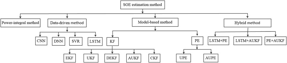
FIGURE 1. SOE estimation method.

A general SOE estimation method is the power integral method (detailed in Mamadou et al. (2012)), in which a new indicator of the energetic reserve, SOE, is proposed to deal with modern BMSs. An improved scheme to estimate the SOE by mapping the relationship between discharge power, remaining energy, and SOE was proposed in Barai et al. (2016). Although this method is advanced to some extent, it needs calibration and is time consuming and expensive.

With the advancements in machine learning methods, the data-driven method has been gaining popularity (Gao and Lu, 2021). Generally, machine learning methods, for example, the genetic algorithm (Hu et al., 2016), neural network (NN) (Hossain et al., 2020), deep neural networks (DNNs) (Hossain et al., 2020), and support vector regression (SVR) (Hu et al., 2014), are widely used for SOE estimation. In Purohit et al. (2021), a method based on a feedforward NN is proposed for the joint estimation of the SOC, SOE, and power loss. The method has been verified by testing, and its prediction accuracy is high. A data-driven method is based on a long short-term memory (LSTM) to jointly estimate the SOC and SOE in Ma et al. (2021). The accuracy and robustness of the method have been verified by the dynamic cycling condition. In Shrivastava et al. (2021), two different data-driven SOE estimation methods, that is, using the DNN and SVR, are compared. The SOE estimation results demonstrate the high accuracy of the DNN over SVR under the same dynamic operating conditions. He et al. (2022) proposed a method based on a radial basis function (RBF) neural network to estimate the energy recovered and the actual energy released when the battery current direction changes. The results show that this method can effectively improve SOE estimation accuracy.

The model-based method uses a resistor–capacitance equivalent circuit model (Zhai et al., 2017; Li et al., 2018; Qin et al., 2019; Wang et al., 2019; Xu et al., 2019), which mainly includes particle filter and Kalman filter families. An unscented particle filter (PF) is used in Chang et al. (2020) to solve the non-linear and noise problems of the system. The experimental results show that the error of the SOE is less than 1.8%. In Zhang et al. (2021), to ensure a precise estimate of the SOE, dual adaptive particle filters are proposed based on the third-order resistor–capacitance equivalent model (TRCEM). Through the dynamic stress test and supplemental federal test, the feasibility and effectiveness of the method are verified. In Hou et al. (2022), using the second-order resistor–capacitance equivalent model (SRCEM), the SOE is estimated based on an adaptive unscented Kalman filter (AUKF) algorithm. The simulation results indicate that the proposed method is adaptive, regardless of whether the initial SOE value is consistent with the real value, and shows high accuracy. A joint estimation method of the maximum available energy and SOE that adopted the Kalman filter algorithm is proposed in Zhang, S., et al. (2021) and Zhang, S.; Zhang, X (2021). The experimental results show that the method has good accuracy and robustness. In Zhou et al. (2021), a method based on a fifth-order simplex square radius cubature Kalman filter is developed to achieve SOE estimation accuracy and robustness. The error of SOE estimation is less than 3%. In Shrivastava et al. (2022), a multiple timescale dual-extended Kalman filter is used to simultaneously estimate the SOC, SOE, state of power (SOP), and SOH, and the experimental results show that the errors of the estimated SOC and SOE are all less than 1%.

It can be seen from the aforementioned literature that a single method has a limited effect on improving the accuracy of SOE estimation, and increasingly more scholars are trying hybrid methods. In Fan et al. (2022), the LSTM combined with an AUKF method is proposed to estimate the SOC and SOE simultaneously. The test results show that the proposed method can effectively estimate the SOC and SOE of LIBs with high accuracy and low complexity. In Lai et al. (2021), the SOE method based on a particle filter and an extended Kalman filter is presented. The experimental results show that the maximum error of SOE estimation is less than 3%. In Chen et al. (2021), an approach for battery SOE prediction is proposed based on an adaptive square root unscented Kalman filter. Owing to the strong non-linear characteristics of LIBs, even with a 20% initial SOE error, the predicted SOE can converge to the actual value. The estimation error of LIB’s SOE is less than 2%. A method based on the extended Kalman filter algorithm and Markov chain model was advanced in An et al. (2022) to predict the future output power, as well as SOE. The results show that this method has high precision and good robustness.

Researchers have not only worked to improve the SOE estimation accuracy but have also studied the adaptability of SOE estimation. In Rahimifard et al. (2021), an online adaptive estimation method is proposed that can achieve a high-precision estimation of the SOC, SOH, and SOP. The effectiveness and accuracy of this method have been verified in a BMS. In Li et al. (2021), an adaptive SOE estimation method based on a cubature Kalman filter applied to series-connected LIB packs is proposed. Even if the initial error is large, in this method, it can be adjusted quickly and has high accuracy; in other words, the root mean square error is less than 2.2%. Both the single SOE (Zhang, S., et al., 2021; Zhang, S.; Zhang, X.; 2021; Fan et al., 2022; Hou et al., 2022) and hybrid SOE estimation methods (Chen et al., 2021) enhance the adaptability and accuracy of the algorithm.

Owing to the performance attenuation of a EULIB, both the Ohmic internal resistance (OIR) and actual energy (AE) have different variations. Accurate estimation is needed to ensure accurate SOE estimation. At the same time, when an error occurs between the actual and initial energy, the estimation method should be able to quickly adjust, track the actual SOE, and have self-adaptability.

To improve the accuracy and adaptability of SOE estimation, in the paper, we study the energy state estimation of a EULIB. First, the four-order resistor–capacitance equivalent model of a EULIB is established, and an unscented transformation is introduced to further improve the estimation accuracy of SOE. Second, a EULIB’s SOE is estimated based on an AUKF, and the OIR and AE of a EULIB are estimated based on the AUKF. Third, a Takagi–Sugeno (TS) fuzzy model is introduced to optimize the OIR and AE of the EULIB, and the SOE estimation method is established based on an adaptive dual unscented Kalman filter (ADUKF). Finally, the accuracy and adaptability of the algorithm are verified and compared in simulation experiments.

The objective of the present study is to propose an SOE estimation method for EULIBs and verify the superiority of the ADUKF. The original contributions of this paper are as follows.

1) The accuracy of SOE estimation is improved, and a four-order resistor–capacitance equivalent model (FRCEM) of a EULIB is established.

2) The TS fuzzy model is introduced to optimize the OIR and AE of the EULIB and to improve the accuracy of SOE estimation.

3) The unscented transformation (UT) is introduced to establish the SOE estimation method based on the ADUKF, and the EULIB’s SOE is estimated based on the AUKF, as is its OIR and AE.

2 Estimation model of the state of energy

2.1 State of energy

Compared with the SOC, the estimation of the SOE increases the influence of the working voltage, which is of great significance in the safety evaluation of EULIBs. The SOE of a EULIB is defined as the ratio of the remaining energy to the maximum available energy and is a direct expression of the remaining available mileage of a EULIB, which can be derived as follows:

$S_{ek+1}=S_{ek}-\frac{U_k∆t}{E}{i}_k,(1)$

where $S_{ek}$ and $S_{ek+1}$ are the SOE of EULIB at k and k + 1 time in a discrete state, respectively; $E$ is the energy of a EULIB; $i_k$ and $U_k$ are the current and working voltage of a EULIB at k time in a discrete state; and $∆t$ is the sampling period.

2.2 State of energy estimation model based on the FRCEM

Owing to the complex non-linear system of a EULIB, in order to simulate the characteristics of a EULIB more accurately, a higher-order battery equivalent model is required.

The FRCEM not only fully considers the influence of the polarization impedance of the EULIB on the performance, but also can reflect the state information of the EULIB in timely and accurate manner. The model has high accuracy and is easy to implement. However, the higher-order resistor–capacitance (RC) model is highly complex and has high requirements on the system, so it is difficult to apply. On the premise of considering accuracy, complexity, and practical value, the FRCEM is adopted in this article.

In Figure 2, $U_{oc}$ is the open-circuit voltage (OCV) of the battery; $U_L$ is the working voltage of the EULIB; $R_{0,U}$ is the ohmic internal resistance of the EULIB; $R_1,R_2,R_3,$ and $R_4$ are the polarization resistance; $C_1,C_2,C_3,$ and $C_4$ are the polarization capacitance; $U_1$, $U_2,$ $U_3,$ and $U_4$ are the voltages at both ends of capacitors $C_1$, $C_2,$ $C_3$, and $C_4$, respectively; $i_L$ is the charge/discharge current; and ${\tau }_1=R_1{C}_1$, ${\tau }_2=R_2{C}_2$, ${\tau }_3=R_3{C}_3$, and ${\tau }_4=R_4{C}_4$ are time constants.

FIGURE 2

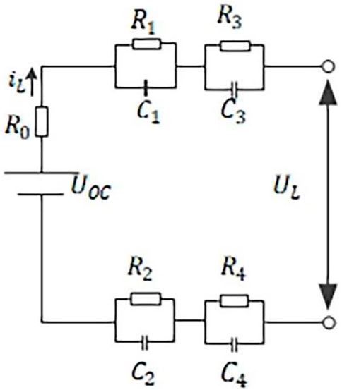
FIGURE 2. FRCEM of SOE estimation.

According to Figure 2, the discrete state equation of EULIB’s FRCEM is as follows:

$\left[\begin{array}{c}{S}_{ek+1}\\ U_{k+1}^{R_1{C}_1}\\ U_{k+1}^{R_2{C}_2}\\ U_{k+1}^{R_3{C}_3}\\ U_{k+1}^{R_4{C}_4}\end{array}\right]=\left[\begin{array}{c}1\\ 0\\ 0\\ 0\\ 0\end{array}\begin{array}{c}0\\ \mathit{exp}\left(-\frac{∆t}{{\tau }_1}\right)\\ 0\\ 0\\ 0\end{array}\begin{array}{c}0\\ 0\\ \mathit{exp}\left(-\frac{∆t}{{\tau }_2}\right)\\ 0\\ 0\end{array}\begin{array}{c}0\\ 0\\ 0\\ \mathit{exp}\left(-\frac{∆t}{{\tau }_3}\right)\\ \mathit{exp}\left(-\frac{∆t}{{\tau }_4}\right)\end{array}\right]\bullet \left[\begin{array}{c}{S}_{ek}\\ U_k^{R_1{C}_1}\\ U_k^{R_2{C}_2}\\ U_k^{R_3{C}_3}\\ U_k^{R_4{C}_4}\end{array}\right]+\left[\begin{array}{c}-\frac{U_k∆t}{E}\\ R_1(1-\mathit{exp}\left(-\frac{∆t}{{\tau }_1}\right))\\ R_2(1-\mathit{exp}\left(-\frac{∆t}{{\tau }_2}\right))\\ R_3(1-\mathit{exp}\left(-\frac{∆t}{{\tau }_3}\right))\\ R_4(1-\mathit{exp}\left(-\frac{∆t}{{\tau }_4}\right))\end{array}\right]\bullet i_k+q_k.(2)$

According to Figure 2, the discrete observation equation of EULIB’s FRCEM is as follows:

$U_k=\left[\frac{d\left(U_{oc}\left(S_e\right)\right)}{d{S}_e}\right.{|}_{S_e=S_{ek}}-1-1\left.-1-1\right]\bullet \left[\begin{array}{c}{S}_{ek}\\ U_k^{R_1{C}_1}\\ U_k^{R_2{C}_2}\\ U_k^{R_3{C}_3}\\ U_k^{R_4{C}_4}\end{array}\right]-i_k{R}_{0,U}+{\gamma }_k.(3)$

As

$A_k=\left[\begin{array}{c}1\\ 0\\ 0\\ 0\\ 0\end{array}\begin{array}{c}0\\ \mathit{exp}\left(-\frac{∆t}{{\tau }_1}\right)\\ 0\\ 0\\ 0\end{array}\begin{array}{c}0\\ 0\\ \mathit{exp}\left(-\frac{∆t}{{\tau }_2}\right)\\ 0\\ 0\end{array}\begin{array}{c}0\\ 0\\ 0\\ \mathit{exp}\left(-\frac{∆t}{{\tau }_3}\right)\\ \mathit{exp}\left(-\frac{∆t}{{\tau }_4}\right)\end{array}\right],B_k=\left[\begin{array}{c}-\frac{U_k∆t}{E}\\ R_1(1-\mathit{exp}\left(-\frac{∆t}{{\tau }_1}\right))\\ R_2(1-\mathit{exp}\left(-\frac{∆t}{{\tau }_2}\right))\\ R_3(1-\mathit{exp}\left(-\frac{∆t}{{\tau }_3}\right))\\ R_4(1-\mathit{exp}\left(-\frac{∆t}{{\tau }_4}\right))\end{array}\right],x_k=\left[\begin{array}{c}{S}_{ek}\\ U_k^{R_1{C}_1}\\ U_k^{R_2{C}_2}\\ U_k^{R_3{C}_3}\\ U_k^{R_4{C}_4}\end{array}\right],{u_k=i}_k,C_k=\left[\frac{d\left(U_{oc}\left(S_e\right)\right)}{d{S}_e}\right.{|}_{S_e=S_{ek}}-1\left.-1-1-1\right]$

So,

$f\left(x_k,u_k\right)=A_k{x}_k+B_k{u}_k,(4)$

$g\left(x_k,u_k\right)=C_k{x}_k-R_{0,k,U}{u}_k,(5)$

where $U_k^{R_1{C}_1}$ $U_k^{R_2{C}_2}$, $U_k^{R_3{C}_3}$, and $U_k^{R_4{C}_4}$ are the estimated voltage values of $R_1$, $R_2,$ $R_3,$ and $R_4$ at k time in a discrete state, respectively; $U_{k+1}^{R_1{C}_1}$ $U_{k+1}^{R_2{C}_2}$, $U_{k+1}^{R_3{C}_3}$, and $U_{k+1}^{R_4{C}_4}$ are the estimated voltage values of $R_1$, $R_2,$ $R_3,$ and $R_4$ at k+1 time in a discrete state, respectively; $q_k,{\gamma }_k$ are independent system noises; $U_{oc}\left(S_e\right)$ is the OCV of a EULIB corresponding to the SOE value of a EULIB at k time in a discrete state.

2.3 Model parameter identification

The working voltage $U_L$, charge/discharge current $i_L$, and the OCV $U_{\mathrm{O}\mathrm{C}}$ of the EULIB are collected through the charge/discharge test. Model parameter identification based on the least square method is not repeated in this article because the method is described in detail in Hou, et al. (2014) and Hou, et al. (2017). Both $U_{OC}$ and $R_{0,U}$ adopt the off-line identification method (Hou et al., 2021; Hou et al., 2022).

3 SOE estimation of the EULIB

In this paper, UT is introduced and the ADUKF algorithm is used to estimate the SOE and OIR and AE, respectively, which are optimized by the TS fuzzy model. The estimation accuracy and adaptability characteristics are compared and analyzed (Ma et al., 2022; Hou, E., et al., 2022).

3.1 UT

UT is the core technology of the unscented Kalman filter (UKF). The UT’s idea is to approximate the distribution of a probability density function through a set of carefully selected sample points and the corresponding weights of the sample points. A certain number of sigma points are selected from the prior distribution, according to a certain strategy, and non-linear transformation is performed on each sigma point to obtain the corresponding transformed sampling points. In addition, the posterior mean and variance are calculated by weighting these sample points. The sample points obtained by UT are neither linearized nor have lost their higher-order terms, so the accuracy of UT is higher than that of the extended Kalman filter algorithm (Hou, et al., 2022).

For any non-linear function $y=\mathrm{g}\left(x\right)$, around the n-dimensional state variable $x$ with the mean value of $\overline{x}$ and variance of $P_x$, 2n +1 sigma points ${\chi }_i$ and corresponding weights ${\omega }_i$ can be selected by the following UT process:

${\chi }_i=\overline{x}i=0$

${\chi }_i=\overline{x}+{\left(\sqrt{\left(n+\lambda \right)P_x}\right)}_{i}i=1,\dots ,n$

${\chi }_i=\overline{x}-{\left(\sqrt{\left(n+\lambda \right)P_x}\right)}_{i-n}i=n+1,\dots ,2n(6)$

${\omega }_0^m={\omega }_0^c=\frac{\lambda }{n+\lambda }i=0$

${\omega }_i^m={\omega }_i^c=\frac{\lambda }{2n+\lambda }i=1,\dots ,2n$

In the aforementioned formula, ${\left(\sqrt{\left(n+\lambda \right)P_x}\right)}_i$ is the $i$ column or row of the square root of $\left(n+\lambda \right)P_x$. $\lambda$ is the scale factor used to represent the range of sampling points around equilibrium value points, and ${\omega }_i^m$ is the weight of the corresponding sample points. In this paper, $\lambda =0.1,i=4$.

From ${\chi }_i$, the sample point with non-linear transformation can be obtained:

$y_i=f\left({\chi }_i\right).(7)$

Then, statistical characteristics of the output sampling points can be obtained by weighted approximation:

$y={\displaystyle \sum }_i^{2n}{\omega }_i^m{y}_i,(8)$

$P_y={\displaystyle \sum }_i^{2n}{\omega }_i^c\left(y_i-y\right){\left(y_i-y\right)}^T.(9)$

3.2 State of energy estimation based on the AUKF

From Eqs 04 and 05, the variable of a EULIB system is the SOE. The state and observation are as follows:

$x_{k+1,U}=f\left(x_{k,U},u_{k,U},{\theta }_{k,U}\right)+q_{k,U},(10)$

$y_{k+1,U}=g\left(x_{k,U},u_{k,U},{\theta }_{k,U}\right)+{\gamma }_{k,U},(11)$

where ${\theta }_{k,u}$ is the state variable OIR and AE, ${\theta }_{k,u}=\left[R_{0,k,u},E_{k,u}\right]$, $x_{k,U}$ is the system state variable of a EULIB; $u_{k,U}$ and $y_{k,U}$ are the input and observation variables of the system, which are the current and the working voltages of a EULIB, respectively; $q_{k,U}and{\gamma }_{k,U}$ are the zero-mean Gaussian white noise, the error covariance matrices of $q_{k,U}and{\gamma }_{k,U}$ are $Q_{k,U}and{R}_{k,U}$.

The AUKF algorithm is as follows:

Step 1:. Initialize $x_{k,U}$:

${\widehat{x}}_{0,U}=E\left(x_{0,U}\right),(12)$

${\widehat{P}}_{0,U}=E[\left(x_{0,U}-{\widehat{x}}_{0,U}\right){\left(x_{0,U}-{\widehat{x}}_{0,U}\right)}^T.(13)$

Step 2:. Generating sigma points:

${\chi }_{i,U}=\left[\overline{x},\overline{x}+{\left(\sqrt{\left(n+\lambda \right)P_x}\right)}_i,\overline{x}-{\left(\sqrt{\left(n+\lambda \right)P_x}\right)}_{i-n}\right].(14)$

Step 3:. Time update of $x_{k,U}$:

${\chi }_{i.k,U}=f\left({\chi }_{i.k-1,U}\right),(15)$

$x_{k,U}={\displaystyle \sum }_{i=0}^{2n}{\omega }_i^m{\chi }_{i.k,U}+q_{k,U},(16)$

$P_{k,U}={\displaystyle \sum }_{i=0}^{2n}{\omega }_i^c\left[{\chi }_{i.k,U}-x_{k,U}\right]{\left[{\chi }_{i.k,U}-x_{k,U}\right]}^T+Q_{k,U},(17)$

$y_{i,k,U}=g\left({\chi }_{i.k-1,U}\right),(18)$

$y_{k,U}={\displaystyle \sum }_{i=0}^{2n}{\omega }_i^m{y}_{i.k,U}+{\gamma }_{k,U},(19)$

$P_{y,k,U}={\displaystyle \sum }_{i=0}^{2n}{\omega }_i^c\left[y_{i.k,U}-y_{k,U}\right]{\left[y_{i.k,U}-y_{k,U}\right]}^T+R_{k,U},(20)$

$P_{xy,k,U}={\displaystyle \sum }_{i=0}^{2n}{\omega }_i^c\left[{\chi }_{i.k,U}-x_{k,U}\right]{\left[y_{i.k,U}-y_{k,U}\right]}^T.(21)$

Step 4:. Status update of $x_{k,U}$:The Kalman gain can be expressed as follows:

$K_{k,U}=P_{xy,k,U}{P}_{y,k,U}^{-1}.(22)$

The optimal estimation of the state variable can be expressed as follows:

${\widehat{x}}_{k,U}=x_{k,U}+K_{k,U}\left[y_{k,U}-{\widehat{y}}_{k,U}\right].(23)$

The optimal estimate of the covariance is as follows:

${\widehat{P}}_{k,U}=P_{k,U}-K_{k,U}{P}_{y,k,U}{K}_{k,U}^T.(24)$

Step 5:. Process noise covariance equation:

$Q_{k,U}=\left(1-d_{k,U}\right)Q_{k-1,U}+d_{k,U}\left[K_{k,U}\left({\widehat{y}}_{k,U}-y_{k,U}\right){\left({\widehat{y}}_{k,U}-y_{k,U}\right)}^T{K}_{k,U}^T+P_{k,U}-A_{k-1,U}{\widehat{P}}_{k-1,U}{A}_{k-1,U}^T\right].(25)$

Step 6:. Observation noise covariance equation:

$R_{k,U}=\left(1-d_{k,U}\right)R_{k-1,\mathrm{U}}+d_{k,U}\left[\left({\widehat{y}}_{k,U}-y_{k,U}\right){\left({\widehat{y}}_{k,U}-y_{k,U}\right)}^T-{C_{k,U}{P}_{k,U}C}_{k,U}^T\right],(26)$

where $d_{k,U}=\frac{1-b_U}{1-b_U^k},k=\mathrm{1,2},\cdots ,n$, $b_U$ is the forgetting factor, 0< $b_U$ <1; $x_{k,U}$ and ${\widehat{x}}_{k,U}$ are the estimation and optimal estimation of the state variable at k time, respectively; $y_{k,U}$ and ${\widehat{y}}_{k,U}$ are the estimated value and actual observation value at k time, respectively; $P_{k,U}$ and${\widehat{P}}_{k,U}$ are, respectively, the estimation and optimal estimation of the error covariance at k time. The subscript U in the formula represents the algorithm formula of the AUKF.According to equations 2, 3, and 23,

${\widehat{x}}_{k,U}=\left[\begin{array}{c}{\widehat{S}}_{ek,U}\\ {\widehat{U}}_{k,U}^{R_1{C}_1}\\ {\widehat{U}}_{k,U}^{R_2{C}_2}\\ {\widehat{U}}_{k,U}^{R_3{C}_3}\\ {\widehat{U}}_{k,U}^{R_4{C}_4}\end{array}\right],(27)$

where ${\widehat{S}}_{ek,U}$ is the optimal value of the SOE based on the AUKF.

3.3 OIR and AE estimation based on the AUKF

The state and observation formulas of the system with the newly added state parameters are as follows:

${\theta }_{k+1,u}={\theta }_{k,u}+q_{\theta ,k,u},(28)$

$D_{k+1,u}=g\left(x_{k,u},u_{k,u},{\theta }_{k,u}\right)+{\gamma }_{\theta ,k,u},(29)$

where $q_{\theta ,k,u}$ is the noise on the input variable, and it is the zero-mean Gaussian white noise; ${\gamma }_{\theta ,k,u}$ is the noise on the output variable, and it is the zero-mean Gaussian white noise; the error covariance matrices of $q_{\theta ,k,u}and{\gamma }_{\theta ,k,u}$ are $Q_{\theta ,k,u}and{R}_{\theta ,k,u}$, respectively; the state variable ${\theta }_{k,u}$ is estimated based on the AUKF algorithm, and the estimated values of the EULIB’s OIR and AE are calculated. In order to improve the accuracy, the error between the actual value and the estimated value of the working voltage is optimized.

The AUKF algorithm flow is as follows:

Step 1:. Initialize $x_{k,U}$:

${\widehat{\theta }}_{0,u}=E\left({\theta }_{0,u}\right),(30)$

$P_{\theta ,0,u}=E\left[\left(x_{0,u}-{\widehat{x}}_{0,u}\right){\left(x_{0,u}-{\widehat{x}}_{0,u}\right)}^T\right].(31)$

Step 2:. Generating sigma points:

${\chi }_{\theta i,u}=\left[\overline{x},\overline{x}+{\left(\sqrt{\left(n+\lambda \right)P_{\theta ,u}}\right)}_i,\overline{x}-{\left(\sqrt{\left(n+\lambda \right)P_{\theta ,u}}\right)}_{i-n}\right].(32)$

Step 3:. Time update of $x_{k,U}$:

${\chi }_{\theta i.k,u}=f\left({\chi }_{\theta i.k-1,u}\right),(33)$

${\theta }_{k.u}={\displaystyle \sum }_{i=0}^{2n}{\omega }_{\theta i}^m{\chi }_{\theta i.k,u}+q_{\theta ,k,u},(34)$

$P_{\theta ,k,u}={\widehat{P}}_{\theta ,k-1,u}+Q_{\theta ,k,u},(35)$

$y_{\theta i,k,u}=g\left({\chi }_{\theta i.k-1,u}\right),(36)$

$y_{\theta ,k,u}={\displaystyle \sum }_{i=0}^{2n}{\omega }_{\theta i}^m{y}_{\theta i.k,u}+{\gamma }_{\theta ,k,u},(37)$

$P_{\theta y,k,u}={\displaystyle \sum }_{i=0}^{2n}{\omega }_{\theta i}^c\left[y_{\theta i.k}-y_{\theta ,k}\right]{\left[y_{\theta i.k}-y_{\theta ,k}\right]}^T+R_{\theta ,k,u},(38)$

$P_{\theta xy,k,u}={\displaystyle \sum }_{i=0}^{2n}{\omega }_{\theta i}^c\left[{\chi }_{\theta i.k,u}-{\theta }_{k.u}\right]{\left[y_{\theta i.k,u}-y_{\theta ,k,u}\right]}^T.(39)$

Step 4:. Status update of $x_{k,U}$:The Kalman gain is as follows:

$K_{\theta ,k,u}=P_{\theta xy,k,u}{P}_{\theta y,k,u}^{-1}.(40)$

The optimal estimation of the state variable is as follows:

${\widehat{\theta }}_{k,u}={\theta }_{k,u}+K_{\theta ,k,u}\left[y_{k,u}-{\widehat{y}}_{k,u}\right].(41)$

The optimal estimate of the covariance is as follows:

${\widehat{P}}_{\theta ,k,u}=P_{\theta ,k,u}-K_{\theta ,k,u}{P}_{\theta y,k,u}{K}_{\theta ,k,u}^T.(42)$

Step 5:. Process noise covariance equation:

$q_{\theta ,k,u}=\left(1-d_{\theta ,k,u}\right)q_{\theta ,k-1,u}+d_{\theta ,k,u}\left[{\widehat{\theta }}_{k,u}-{\displaystyle \sum }_{i=0}^{2n}{\omega }_{\theta i}^{m}f\left({\chi }_{\theta i.k-1,u},u_{k,u},{\theta }_k,u\right)\right],(43)$

$Q_{\theta ,k,u}=\left(1-d_{\theta ,k,u}\right)Q_{\theta ,k-1,u}+d_{\theta ,k,u}\left[K_{\theta ,k,u}\left({\widehat{y}}_{k,u}-y_{k,u}\right){\left({\widehat{y}}_{k,u}-y_{k,u}\right)}^T{K}_{\theta ,k,u}^T+P_{\theta ,k,u}-A_{k-1,u}{\widehat{P}}_{\theta ,k-1,u}{A}_{k-1,u}^T\right].(44)$

Step 6:. Observation of the noise covariance equation:

${\gamma }_{\theta ,k,u}=\left(1-d_{\theta ,k,u}\right){\gamma }_{\theta ,k-1,u}+d_{\theta ,k,u}\left[y_{\theta ,k,u}-{\displaystyle \sum }_{i=0}^{2n}{\omega }_{\theta i}^{m}g\left({\chi }_{\theta i.k-1}\right)\right],(45)$

$R_{\theta ,k,u}=\left(1-d_{\theta ,k,u}\right)R_{\theta ,k-1,u}+d_{\theta ,k,u}\left[\left({\widehat{y}}_{k,u}-y_{k,u}\right){\left({\widehat{y}}_{k,u}-y_{k,u}\right)}^T-{C_{k,u}{P}_{\theta ,k,u}C}_{k,u}^T\right],(46)$

where $d_{\theta ,k,u}=\frac{1-b_{\theta ,u}}{1-b_{\theta ,u}^k}$, and $b_{\theta }$ is the forgetting factor of $\theta$, 0 < $b_{\theta ,k,u}$ < 1 , $k=\mathrm{1,2},\cdots ,n$.

3.4 OIR based on TS fuzzy optimization

In order to further improve the estimation accuracy of the SOE, this paper adopts the TS fuzzy model to the OIR and AE in the Kalman filter process (Hou, E., et al., 2022).

The OIR $R_{0,U}$ theory domain: [1 3].

The OIR $R_{0,U}$ fuzzy language variables: $R_L$, $R_M$, and $R_H$.

The OIR $R_{0,U}$ membership function expression:

${\mu }_{R_L}=\mathit{exp}\left(-\frac{{\left(s-1\right)}^2}{2*2^2}\right),(47)$

${\mu }_{R_M}=\mathit{exp}\left(-\frac{{\left(s-2\right)}^2}{2*2^2}\right),(48)$

${\mu }_{R_H}=\mathit{exp}\left(-\frac{{\left(s-3\right)}^2}{2*2^2}\right).(49)$

Definition:

$∆R_{0,k,U}=R_{0,k,U}-R_{0,k-1,U}.(50)$

The change rate of the OIR $∆R_{0,k,U}$ theory domain: [−0.3 0.6].

The change rate of OIR $∆R_{0,k,U}$ fuzzy language variables: ${∆R}_L$, ${∆R}_M$, and $∆R_H$.

The change rate of OIR $∆R_{0,k,U}$ membership function expression:

${\mu }_{∆R_L}=\mathit{exp}\left(-\frac{{\left(s+0.3\right)}^2}{2*{0.6}^2}\right),(51)$

${\mu }_{∆R_M}=\mathit{exp}\left(-\frac{{\left(s-0.1\right)}^2}{2*{0.6}^2}\right),(52)$

${\mu }_{∆R_H}=\mathit{exp}\left(-\frac{{\left(s-0.4\right)}^2}{2*{0.6}^2}\right).(53)$

According to Table 1, the optimal updated value of OIR is as follows:

${\widehat{R}}_{0,k,U}=\frac{{\displaystyle \sum }_{i=1}^9{\mu }^i{f}_{Ri}}{{\displaystyle \sum }_{i=1}^9{\mu }^i},(54)$

where $n=9$ is the number of fuzzy rules, $f_{Ri}$ is the conclusion equation from rule $i$, and ${\mu }^i$ represents the membership degree of rule $i$ corresponding to this generalized input vector.

TABLE 1

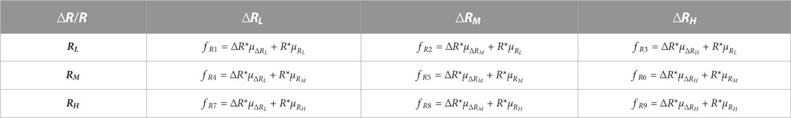
TABLE 1. Fuzzy optimization decision table for the OIR.

3.5 AE based on TS fuzzy optimization

The AE $E_{0,U}$ theory domain: [44 66].

The AE $E_{0,U}$ fuzzy language variables: $E_L$, $E_M$, and $E_H$.

The AE $E_{0,U}$ membership function expression:

${\mu }_{E_L}=\mathit{exp}\left(-\frac{{\left(s-45\right)}^2}{2*{10}^2}\right),(55)$

${\mu }_{E_M}=\mathit{exp}\left(-\frac{{\left(s-55\right)}^2}{2*{10}^2}\right),(56)$

${\mu }_{E_H}=\mathit{exp}\left(-\frac{{\left(s-60\right)}^2}{2*{10}^2}\right),(57)$

$∆E_{0,k,U}=E_{0,k,U}-E_{0,k-1,U}.(58)$

The change rate of the AE $∆E_{0,k,U}$ theory domain: [−30 50].

The change rate of AE $∆E_{0,k,U}$ fuzzy language variables: ${∆E}_L$, ${∆E}_M$, and $∆E_H$.

The change rate of AE $∆E_{0,k,U}$ membership function expression:

${\mu }_{{∆E}_L}=\mathit{exp}\left(-\frac{{\left(s+20\right)}^2}{2*{10}^2}\right),(59)$

${\mu }_{{∆E}_M}=\mathit{exp}\left(-\frac{{\left(s-10\right)}^2}{2*{20}^2}\right),(60)$

${\mu }_{{∆E}_H}=\mathit{exp}\left(-\frac{{\left(s-40\right)}^2}{2*{10}^2}\right).(61)$

According to Table 2, the optimal updated value of AE is as follows:

${\widehat{E}}_{0,k,U}=\frac{{\displaystyle \sum }_{i=1}^9{\mu }^i{f}_{Ei}}{{\displaystyle \sum }_{i=1}^9{\mu }^i},(62)$

where $n=9$ is the number of fuzzy rules, $f_{Ei}$ is the conclusion equation from rule $i$, and ${\mu }^i$ represents the membership degree of rule $i$ corresponding to this generalized input vector.

TABLE 2

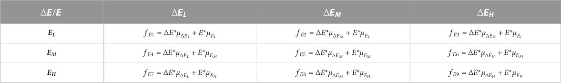
TABLE 2. Fuzzy optimization decision table for AE.

3.6 SOE estimation based on the ADUKF

The SOE estimation flow chart of the EULIB based on the ADUKF is shown in Figure 3.

FIGURE 3

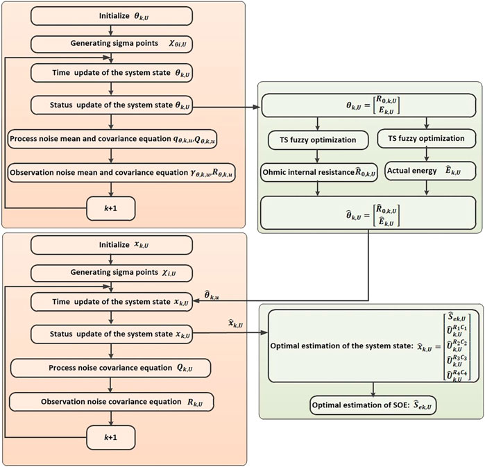
FIGURE 3. SOE estimation flow chart.

4 Simulation and discussion

4.1 Experiment

According to Figure 4 and Table 3, the EULIB is selected to conduct the charge–discharge experiment using test equipment (BTS20) at room temperature. In order to simulate the working conditions, the fully charged EULIB was discharged several times. Different discharge currents were used each time for simulation, verification, and analysis based on MATLAB R2022a.

FIGURE 4

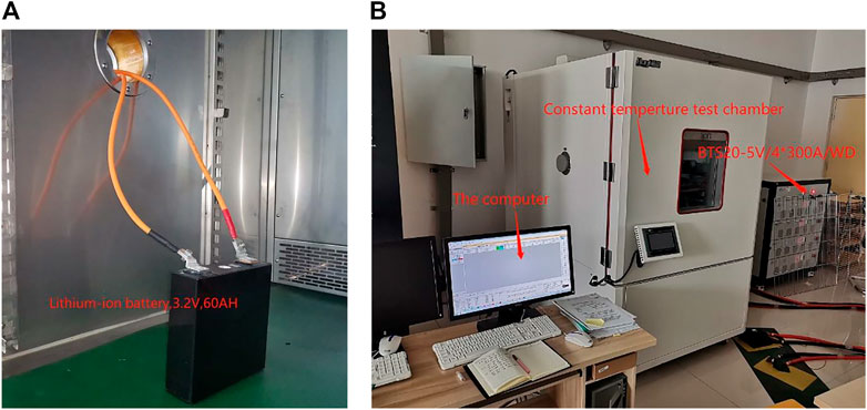
FIGURE 4. Battery testing system. (A) Lithium-ion battery. (B) Charge/discharge experiment (BTS20).

TABLE 3

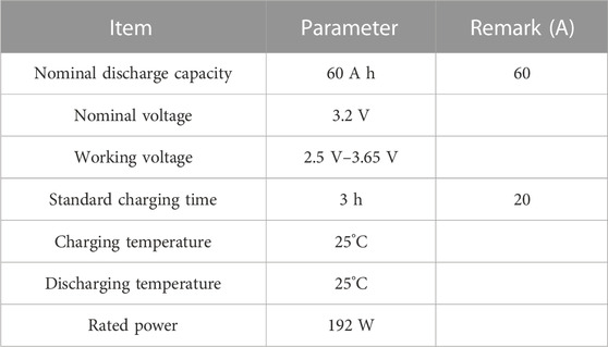
TABLE 3. Parameters of the battery.

In order to verify the adaptive characteristics of the ADUKF algorithm, a test experiment was carried out on a fully charged EULIB, starting from an SOE of 100% to ending at an SOE of 25%. In the paper, selected battery energy decays to 80%, 60%, and 40% separately of rated energy, and the initial SOE values were changed to 100%, 60%, and 20% separately, and the adaptive and error curves were observed and analyzed.

In the process of simulation and verification, the estimated value of the SOE was calculated based on the ADUKF algorithm, and the actual value was acquired by BTS20.

According to Eq. 27, the formula for error is as follows:

The SOE error of the ADUKF formula is as follows:

$OEerrorofADUKF={\widehat{S}}_{ek,U}-S_{actual},(63)$

where $S_{actual}$ is the value acquired by a piece of test equipment.

4.2 Energy decays to 80% and the SOE starts at 100%

The simulation comparative verification curve when energy decays to 80% and the SOE starts at 100% is shown in Figure 5.

FIGURE 5

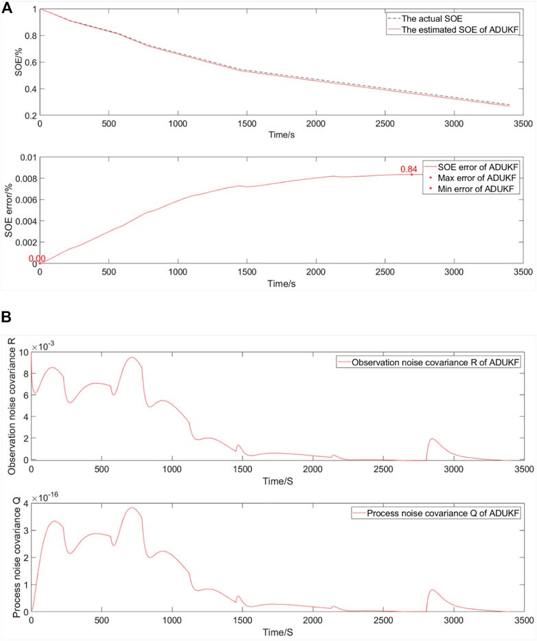
FIGURE 5. Simulation comparative validation curve when energy decays to 80% and the SOE starts at 100%. (A) Estimation and error curves of the SOE. (B) Observation noise covariance R and process noise covariance Q.

The SOE estimation curves of the EULIB are shown in Figure 5A. The bottom graph is the SOE error curve, and the top graph is the SOE adaptive estimation curve. As shown in Table 4 and Figure 5, the SOE error is 0%–0.84% based on the ADUKF with TS fuzzy optimization.

TABLE 4

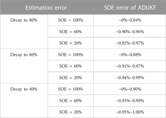
TABLE 4. Estimation error of the EULIB’s SOE.

The observation noise covariance and process noise covariance curves of a EULIB are shown in Figure 5B. The bottom graph is the process noise covariance curve, and the top graph is the observation noise covariance curve.

According to the variation trend of observation and process noise covariance curves, the method is convergent.

4.3 Energy decays to 80% and SOE starts at 60%

The simulation comparative verification curve when energy decays to 80% and the SOE starts at 60% is shown in Figure 6.

FIGURE 6

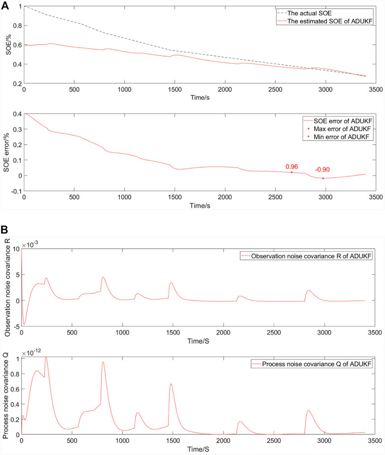
FIGURE 6. Simulation comparative validation curve when energy decays to 80% and the SOE starts at 60%. (A) Estimation and error curves of the SOE. (B) Observation noise covariance R and process noise covariance Q.

The SOE estimation curves of EULIB are shown in Figure 6A. The bottom graph is SOE error curve, and the top graph is the SOE adaptive estimation curve. As shown in Table 4 and Figure 6, the SOE error is −0.90%–0.96% (maximum and minimum errors in the SOE error curve) based on the ADUKF with TS fuzzy optimization.

The observation noise covariance and process noise covariance curves of a EULIB are shown in Figure 6B. The bottom graph is the process noise covariance curve, and the top graph is observation noise covariance curve.

According to the variation trend of observation and process noise covariance curves, the method is convergent. The change in observation noise covariance is small, but the change in process noise covariance is large, compared with that when SOE is 100%. Since the initial value is different, the algorithm is adjusted and the actual value is tracked very high in the end.

4.4 Energy decays to 80% and the SOE starts at 20%

The simulation comparative verification curve when energy decays to 80% and the SOE starts at 20% is shown in Figure 7.

FIGURE 7

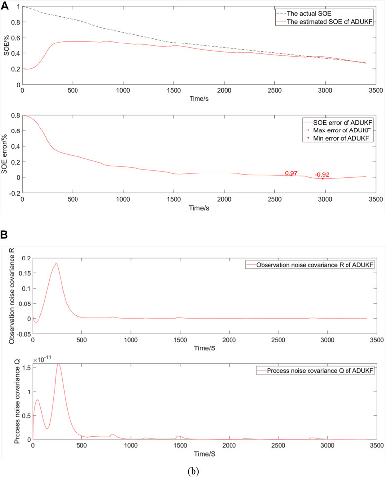
FIGURE 7. Simulation comparative validation curve when energy decays to 80% and the SOE starts at 20%. (A) Estimation and error curves of the SOE. (B) Observation noise covariance R and process noise covariance Q.

The SOE estimation curves of a EULIB are shown in Figure 7A. The bottom graph is the SOE error curve, and the top graph is the SOE adaptive estimation curve. As shown in Table 4 and Figure 7, the SOE error is −0.92%–0.97% (maximum and minimum errors in the SOE error curve) based on the ADUKF with TS fuzzy optimization.

The observation noise covariance and process noise covariance curves of a EULIB are shown in Figure 7B The bottom graph is process noise covariance curve, and the top graph is the observation noise covariance curve.

According to the variation trend of observation and process noise covariance curves, the method is convergent. The changes in observation and process noise covariance are both increased, compared with that when the SOE is 60%. Since the initial value is different, the algorithm is adjusted and the actual value is tracked very high in the end.

4.5 Energy decays to 60% and SOE starts at 100%

The simulation comparative verification curve when energy decays to 60% and the SOE starts at 100% is shown in Figure 8.

FIGURE 8

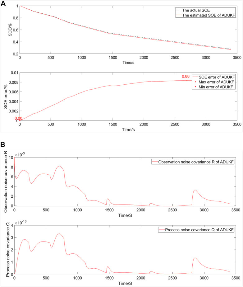
FIGURE 8. Simulation comparative validation curve when energy decays to 60% and the SOE starts at 100%. (A) Estimation and error curves of the SOE. (B) Observation noise covariance R and process noise covariance Q.

The SOE estimation curves of a EULIB are shown in Figure 8A. The bottom graph is the SOE error curve, and the top graph is the SOE adaptive estimation curve. As shown in Table 4 and Figure 8, the SOE error is 0%–0.88% (maximum and minimum errors in the SOE error curve) based on the ADUKF with TS fuzzy optimization.

The observation noise covariance and process noise covariance curves of a EULIB are shown in Figure 8B. The bottom graph is process noise covariance curve, and the top graph is the observation noise covariance curve.

According to the variation trend of observation and process noise covariance curves, the method is convergent. As the energy decays more, the algorithm needs stronger adjustment ability and the error is larger than that before the decays.

4.6 Energy decays to 60% and the SOE starts at 60%

The simulation comparative verification curve when energy decays to 60% and the SOE starts at 60% is shown in Figure 9.

FIGURE 9

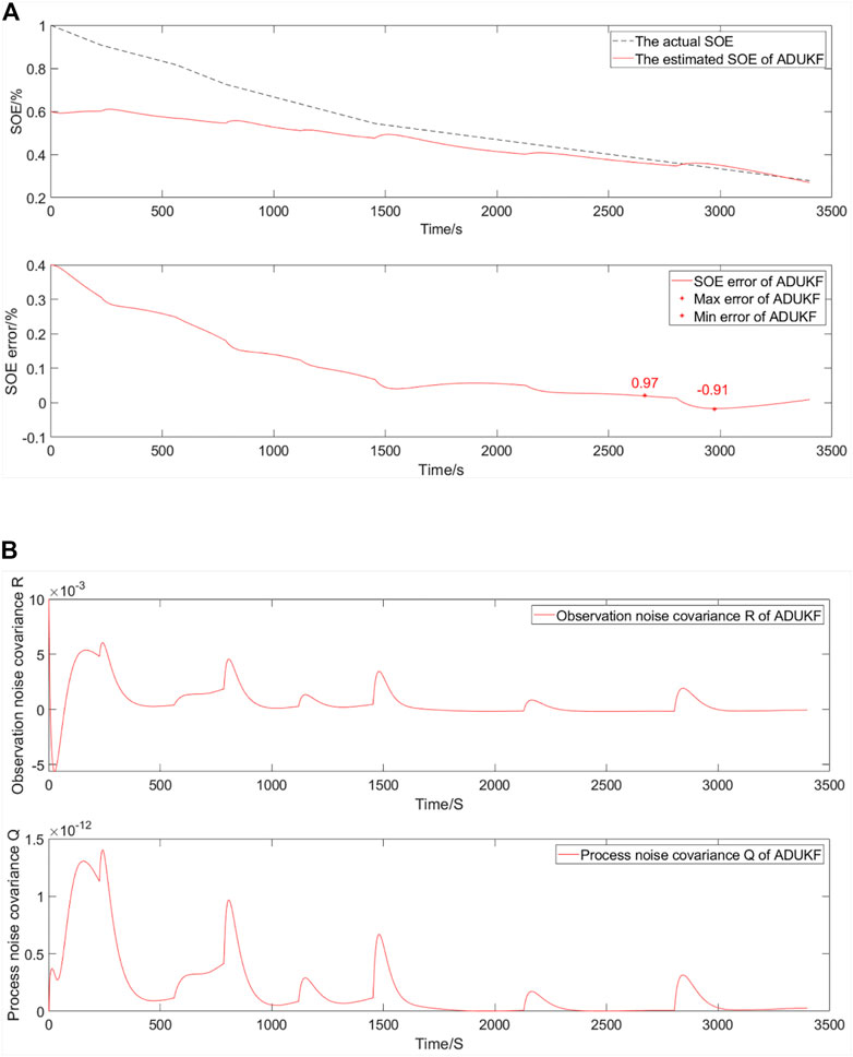
FIGURE 9. Simulation comparative validation curve when energy decays to 60% and the SOE starts at 60%. (A) Estimation and error curves of the SOE. (B) Observation noise covariance R and process noise covariance Q.

The SOE estimation curves of a EULIB are shown in Figure 9A The bottom graph is the SOE error curve, and the top graph is the SOE adaptive estimation curve. As shown in Table 4 and Figure 9, the SOE error is −0.91%–0.97% (maximum and minimum errors in the SOE error curve) based on the ADUKF with TS fuzzy optimization.

The observation noise covariance and process noise covariance curves of a EULIB are shown in Figure 9B. The bottom graph is the process noise covariance curve, and the top graph is the observation noise covariance curve.

According to the variation trend of observation and process noise covariance curves, the method is convergent. With the intensification of energy attenuation, the algorithm needs stronger adjustment ability and the error is larger than that of energy attenuation to 80%. However, tracking the actual value is good.

4.7 Energy decays to 60% and the SOE starts at 20%

The simulation comparative verification curve when energy decays to 60% and the SOE starts at 20% is shown in Figure 10.

FIGURE 10

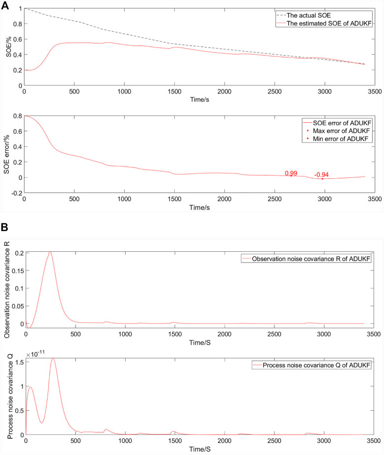
FIGURE 10. Simulation comparative validation curve when energy decays to 60% and the SOE starts at 20%. (A) Estimation and error curves of the SOE. (B) Observation noise covariance R and process noise covariance Q.

The SOE estimation curves of a EULIB are shown in Figure 10A The bottom graph is the SOE error curve, and the top graph is the SOE adaptive estimation curve. As shown in Table 4 and Figure 10, the SOE error is −0.94%–0.99% (maximum and minimum errors in the SOE error curve) based on the ADUKF with TS fuzzy optimization.

The observation noise covariance and process noise covariance curves of a EULIB are shown in Figure 10B The bottom graph is the process noise covariance curve, and the top graph is the observation noise covariance curve.

According to the variation trend of observation and process noise covariance curves, the method is convergent. With the intensification of energy attenuation, the algorithm needs stronger adjustment ability and the error is larger than that of energy attenuation to 80%. However, tracking the actual value is good.

4.8 Energy decays to 40% and the SOE starts at 100%

The simulation comparative verification curve when energy decays to 40% and the SOE starts at 100% is shown in Figure 11.

FIGURE 11

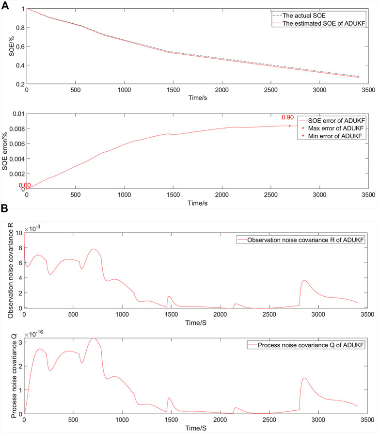
FIGURE 11. Simulation comparative validation curve when energy decays to 40% and the SOE starts at 100%. (A) Estimation and error curves of the SOE. (B) Observation noise covariance R and process noise covariance Q.

The SOE estimation curves of a EULIB are shown in Figure 11A. The bottom graph is the SOE error curve, and the top graph is the SOE adaptive estimation curve. As shown in Table 4 and Figure 11, the SOE error is 0%–0.90% (maximum and minimum errors in the SOE error curve) based on ADUKF with TS fuzzy optimization.

The observation noise covariance and process noise covariance curves of a EULIB are shown in Figure 11B The bottom graph is the process noise covariance curve, and the top graph is the observation noise covariance curve.

According to the variation trend of observation and process noise covariance curves, the method is convergent. As the energy decays more, the algorithm needs stronger adjustment ability and the error is larger than that before the decays.

4.9 Energy decays to 40% and the SOE starts at 60%

The simulation comparative verification curve when energy decays to 40% and the SOE starts at 60% is shown in Figure 12.

FIGURE 12

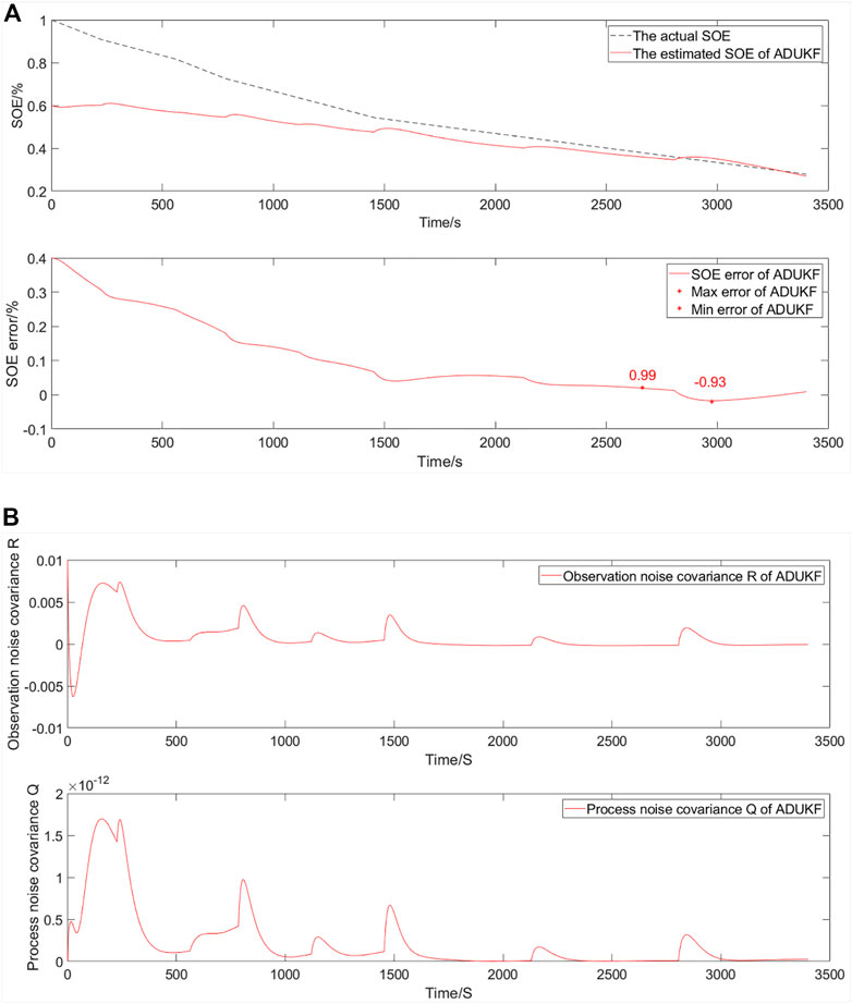
FIGURE 12. Simulation comparative validation curve when energy decays to 40% and the SOE starts at 60%. (A) Estimation and error curves of the SOE. (B) Observation noise covariance R and process noise covariance Q.

The SOE estimation curves of a EULIB are shown in Figure 12A, The bottom graph is the SOE error curve, and the top graph is the SOE adaptive estimation curve. As shown in Table 4 and Figure 12, the SOE error is −0.93%–0.99% (maximum and minimum errors in the SOE error curve) based on the ADUKF with TS fuzzy optimization.

The observation noise covariance and process noise covariance curves of a EULIB are shown in Figure 12B The bottom graph is the process noise covariance curve, and the top graph is the observation noise covariance curve.

According to the variation trend of observation and process noise covariance curves, the method is convergent. With the intensification of energy attenuation, the algorithm needs stronger adjustment ability and the error is larger than that of energy attenuation to 60%. However, tracking the actual value is good.

4.10 Energy decays to 40% and the SOE starts at 20%

The simulation comparative verification curve when energy decays to 40% and the SOE starts at 20% is shown in Figure 13.

FIGURE 13

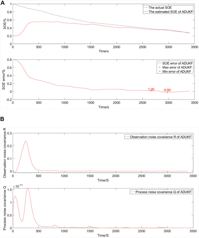
FIGURE 13. Simulation comparative validation curve when energy decays to 40% and the SOE starts at 20%. (A) Estimation and error curves of the SOE. (B) Observation noise covariance R and process noise covariance Q.

The SOE estimation curves of a EULIB are shown in Figure 13A The bottom graph is the SOE error curve, and the top graph is the SOE adaptive estimation curve. As shown in Table 4 and Figure 13, the SOE error is −0.95%–1.00% (maximum and minimum errors in the SOE error curve) based on the ADUKF with TS fuzzy optimization.

The observation noise covariance and process noise covariance curves of a EULIB are shown in Figure 13B. The bottom graph is the process noise covariance curve, and the top graph is the observation noise covariance curve.

According to the variation trend of observation and process noise covariance curves, the method is convergent. With the intensification of energy attenuation, the algorithm needs stronger adjustment ability and the error is larger than that of energy attenuation to 60%. However, tracking the actual value is good.

4.11 Discussion

The simulation results show that the estimation accuracy error of the EULIB’s SOE is less than 1.00% based on a TS fuzzy-optimized ADUKF. With the continuous attenuation of energy, the algorithm is required to have increasingly more adaptive ability, and although the error also increases, the maximum error is less than 1%. As shown in Table 5, compared with the SOE estimation accuracy of 1.8% in Chang et al. (2020), 2% in Chen et al. (2021), 3% in Zhou et al. (2021) and Lai et al. (2021), 2.34% in Hou et al. (2022), and 1% in Shrivastava et al. (2022), the method proposed in this paper has higher accuracy. Furthermore, the proposed method is adaptive, regardless of whether the initial SOE value is consistent with the actual value.

TABLE 5

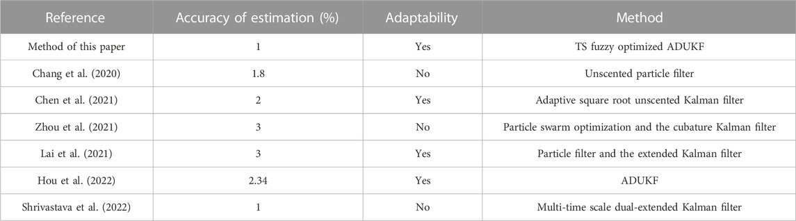
TABLE 5. Comparison of optimization methods.

5 Conclusion

In this paper, the SOE estimation method based on a TS fuzzy optimization ADUKF is established of a EULIB. To improve the accuracy of SOE estimation, the four-order resistor–capacitance equivalent model is used to estimate the SOE, OIR, and AE based on an adaptive dual unscented Kalman filter. To improve the accuracy of the estimation model, the OIR and AE have been optimized based on the TS fuzzy model. To enhance the adaptive ability, the process error and the observation error are estimated. Through simulation, energy decayed to 80%, 60%, and 40% of the rated energy; with the initial value of the SOE starting at 100%, 60%, or 20%, the estimated SOE can track the actual value. The estimation accuracy error of the EULIB’s SOE is less than 1.00% based on a TS fuzzy optimization ADUKF, and the algorithm has higher accuracy.

Also, positive results have been achieved in this paper, both in accuracy and adaptability. However, due to the high-order equivalent model, compared with the low-order model, the calculation amount is larger.

Data availability statement

The original contributions presented in the study are included in the article/Supplementary Material. Further inquiries can be directed to the corresponding author.

Author contributions

EH: writing—original draft preparation, conceptualization, validation, and methodology. ZXW: project administration, funding acquisition, and resources. ZW: writing—review and editing and supervision. XQ: visualization, data curation, and software. GL: formal analysis and investigation. All authors have read and agreed to the published version of the manuscript.

Funding

This work was supported by the Science and Technology Major Project of Inner Mongolia Autonomous Region (2020ZD0014). This research was conducted within the University of Shandong Jiao Tong, supported by the charging discharging equipment BTS20 (5V/4*300A/WD).

Acknowledgments

The authors thank the testing team members for their support with the experiment.

Conflict of interest

The authors declare that the research was conducted in the absence of any commercial or financial relationships that could be construed as a potential conflict of interest.

Publisher’s note

All claims expressed in this article are solely those of the authors and do not necessarily represent those of their affiliated organizations, or those of the publisher, the editors, and the reviewers. Any product that may be evaluated in this article, or claim that may be made by its manufacturer, is not guaranteed or endorsed by the publisher.

References

An, F., Jiang, J., Zhang, W., Zhang, C., and Fan, X. (2022). State of energy estimation for lithium-ion battery pack via prediction in electric vehicle applications. IEEE Trans. Veh. Technol. 71 (1), 184–195. doi:10.1109/tvt.2021.3125194

CrossRef Full Text | Google Scholar

Barai, A., Uddin, K., Widanalage, W. D., McGordon, A., and Jennings, P. (2016). The effect of average cycling current on total energy of lithium-ion batteries for electric vehicles. J. Power Sources 303, 81–85. doi:10.1016/j.jpowsour.2015.10.095

CrossRef Full Text | Google Scholar

Chang, J., Chi, M., and Shen, T. (2020). Model based state-of-energy estimation for LiFePO4 batteries using unscented particle filter. J. Power Electron. 20 (2), 624–633. doi:10.1007/s43236-020-00051-5

CrossRef Full Text | Google Scholar

Chen, Y., Yang, X., Luo, D., and Wen, R. (2021). Remaining available energy prediction for lithium-ion batteries considering electrothermal effect and energy conversion efficiency. J. Energy Storage 40, 102728. doi:10.1016/j.est.2021.102728

CrossRef Full Text | Google Scholar

Fan, T.-E., Liu, S.-M., Tang, X., and Qu, B. (2022). Simultaneously estimating two battery states by combining a long short-term memory network with an adaptive unscented Kalman filter. J. Energy Storage 50, 104553. doi:10.1016/j.est.2022.104553

CrossRef Full Text | Google Scholar

Gao, T., and Lu, W. (2021). Machine learning toward advanced energy storage devices and systems. iScience 24 (1), 101936. doi:10.1016/j.isci.2020.101936

PubMed Abstract | CrossRef Full Text | Google Scholar

He, P., Wang, C., Zhao, W., Wang, W., Wu, G., and Chang, C. (2022). A SOE estimation method for lithium batteries considering available energy and recovered energy. Proc. Institution Mech. Eng. Part D J. Automob. Eng. 237, 273–290. doi:10.1177/09544070211070441

CrossRef Full Text | Google Scholar

Hossain Lipu, M. S., Ansari, S., Miah, M. S., Meraj, S. T., Hasan, K., Shihavuddin, A. S. M., et al. (2022). Deep learning enabled state of charge, state of health and remaining useful life estimation for smart battery management system: Methods, implementations, issues and prospects. J. Energy Storage 55, 105752. doi:10.1016/j.est.2022.105752

CrossRef Full Text | Google Scholar

Hossain Lipu, M. S., Hannan, M. A., Hussain, A., Ayob, A., Saad, M. H. M., Karim, T. F., et al. (2020). Data-driven state of charge estimation of lithium-ion batteries: Algorithms, implementation factors, limitations and future trends. J. Clean. Prod. 277, 124110. doi:10.1016/j.jclepro.2020.124110

CrossRef Full Text | Google Scholar

Hou, E., Qiao, X., and Liu, G. (2017). Estimation of power lithium-ion battery SOC based on fuzzy optimal decision. Chin. J. Power Sources 41, 920–922.

Google Scholar

Hou, E., Qiao, X., and Liu, G. (2014). Modeling and simulation of power lithium-ion battery SOC. Chin. Comput. Simul. 31, 193–196.

Google Scholar

Hou, E., Wang, Z., Qiao, X., and Liu, G. (2022). Remaining useful cycle life prediction of lithium-ion battery based on TS fuzzy model. Front. Energy Res. 10. doi:10.3389/fenrg.2022.973487

CrossRef Full Text | Google Scholar

Hou, E., Xu, Y., Qiao, X., Liu, G., and Wang, Z. (2022). Research on state of power estimation of echelon-use battery based on adaptive unscented kalman filter. Symmetry 14 (5), 919. doi:10.3390/sym14050919

CrossRef Full Text | Google Scholar

Hou, E., Xu, Y., Qiao, X., Liu, G., and Wang, Z. (2021). State of power estimation of echelon-use battery based on adaptive dual extended kalman filter. Energies 14 (17), 5579. doi:10.3390/en14175579

CrossRef Full Text | Google Scholar

Hu, J. N., Hu, J. J., Lin, H. B., Li, X. P., Jiang, C. L., Qiu, X. H., et al. (2014). State-of-charge estimation for battery management system using optimized support vector machine for regression. J. Power Sources 269, 682–693. doi:10.1016/j.jpowsour.2014.07.016

CrossRef Full Text | Google Scholar

Hu, X., Li, S. E., and Yang, Y. (2016). Advanced machine learning approach for lithium-ion battery state estimation in electric vehicles. IEEE Trans. Transp. Electrification 2 (2), 140–149. doi:10.1109/tte.2015.2512237

CrossRef Full Text | Google Scholar

Hu, X., Yuan, H., Zou, C., Li, Z., and Zhang, L. (2018). Co-estimation of state of charge and state of health for lithium-ion batteries based on fractional-order calculus. IEEE Trans. Veh. Technol. 67 (11), 10319–10329. doi:10.1109/tvt.2018.2865664

CrossRef Full Text | Google Scholar

Lai, X., Huang, Y., Han, X., Gu, H., and Zheng, Y. (2021). A novel method for state of energy estimation of lithium-ion batteries using particle filter and extended Kalman filter. J. Energy Storage 43, 103269. doi:10.1016/j.est.2021.103269

CrossRef Full Text | Google Scholar

Li, K., Wei, F., Tseng, K. J., and Soong, B.-H. (2018). A practical lithium-ion battery model for state of energy and voltage responses prediction incorporating temperature and ageing effects. IEEE Trans. Industrial Electron. 65 (8), 6696–6708. doi:10.1109/tie.2017.2779411

CrossRef Full Text | Google Scholar

Li, X., Xu, J., Hong, J., Tian, J., and Tian, Y. (2021). State of energy estimation for a series-connected lithium-ion battery pack based on an adaptive weighted strategy. Energy 214, 118858. doi:10.1016/j.energy.2020.118858

CrossRef Full Text | Google Scholar

Ma, D., Gao, K., Mu, Y., Wei, Z., and Du, R. (2022). An adaptive tracking-extended kalman filter for SOC estimation of batteries with model uncertainty and sensor error. Energies 15 (10), 3499. doi:10.3390/en15103499

CrossRef Full Text | Google Scholar

Ma, L., Hu, C., and Cheng, F. (2021). State of charge and state of energy estimation for lithium-ion batteries based on a long short-term memory neural network. J. Energy Storage 37, 102440. doi:10.1016/j.est.2021.102440

CrossRef Full Text | Google Scholar

Mamadou, K., Lemaire, E., Delaille, A., Riu, D., Hing, S. E., and Bultel, Y. (2012). Definition of a state-of-energy indicator (SoE) for electrochemical storage devices: Application for energetic availability forecasting. J. Electrochem. Soc. 159 (8), A1298–A1307. doi:10.1149/2.075208jes

CrossRef Full Text | Google Scholar

Purohit, K., Srivastava, S., Nookala, V., Joshi, V., Shah, P., Sekhar, R., et al. (2021). Soft sensors for state of charge, state of energy, and power loss in formula student electric vehicle. Appl. Syst. Innov. 4 (4), 78. doi:10.3390/asi4040078

CrossRef Full Text | Google Scholar

Qiao, X., Wang, Z., Hou, E., Liu, G., and Cai, Y. (2022). Online estimation of open circuit voltage based on extended kalman filter with self-evaluation criterion. Energies 15 (12), 4373. doi:10.3390/en15124373

CrossRef Full Text | Google Scholar

Qin, D., Li, J., Wang, T., and Zhang, D. (2019). Modeling and simulating a battery for an electric vehicle based on modelica. Automot. Innov. 2 (3), 169–177. doi:10.1007/s42154-019-000660

CrossRef Full Text | Google Scholar

Rahimifard, S., Ahmed, R., and Habibi, S. (2021). Interacting multiple model strategy for electric vehicle batteries state of charge/health/power estimation. IEEE Access 9, 109875–109888. doi:10.1109/access.2021.3102607

CrossRef Full Text | Google Scholar

Shrivastava, P., Soon, T. K., Idris, M. Y. I. B., Mekhilef, S., and Adnan, S. B. R. S. (2022). Model-based state of X estimation of lithium-ion battery for electric vehicle applications. Int. J. Energy Res. 46, 10704–10723. doi:10.1002/er.7874

CrossRef Full Text | Google Scholar

Shrivastava, P., Tey Kok, S., Yamani Bin Idris, M., Mekhilef, S., and Bahari Ramadzan Syed Adnan, S. (2021). Lithium-ion battery state of energy estimation using deep neural network and support vector regression. doi:10.1109/ECCE-Asia49820.2021.9479413

CrossRef Full Text | Google Scholar

Tran, M. K., Panchal, S., Khang, T. D., Panchal, K., Fraser, R., and Fowler, M. (2022). Concept review of a cloud-based smart battery management system for lithium-ion batteries: Feasibility, logistics, and functionality. Batter. (Basel) 8 (2), 19. doi:10.3390/batteries8020019

CrossRef Full Text | Google Scholar

Wang, Q., Wang, Z., Zhang, L., Liu, P., and Zhou, L. (2022). A battery capacity estimation framework combining hybrid deep neural network and regional capacity calculation based on real-world operating data. IEEE Trans. Industrial Electron., 1–11. doi:10.1109/tie.2022.3229350

CrossRef Full Text | Google Scholar

Wang, S., Chen, Q., Wang, K., Wang, Z., and Wang, Y. (2019). Parameter identification of lithium iron phosphate battery model for battery electric vehicle. IOP Conf. Ser. Mater. Sci. Eng. 677 (3), 032048. doi:10.1088/1757-899x/677/3/032048

CrossRef Full Text | Google Scholar

Wang, S., Fan, Y., Jin, S., Takyi-Aninakwa, P., and Fernandez, C. (2023). Improved anti-noise adaptive long short-term memory neural network modeling for the robust remaining useful life prediction of lithium-ion batteries. Reliab. Eng. Syst. Saf. 230. doi:10.1016/j.ress.2022.108920

CrossRef Full Text | Google Scholar

Xu, W., Xu, J., Lang, J., and Yan, X. (2019). A multi-timescale estimator for lithium-ion battery state of charge and state of energy estimation using dual H infinity filter. IEEE Access 7, 181229–181241. doi:10.1109/access.2019.2959396

CrossRef Full Text | Google Scholar

Yong, F., Fan, B., Chen, X., and Fengling, H. (2021). State-of-Charge and state-of-energy estimation for lithium-ion batteries using sliding-mode observers.

Google Scholar

Zhai, G., Liu, S., Wang, Z., Zhang, W., and Ma, Z. (2017). State of energy estimation of lithium titanate battery for rail transit application. Energy Procedia 105, 3146–3151. doi:10.1016/j.egypro.2017.03.681

CrossRef Full Text | Google Scholar

Zhang, S., Peng, N., and Zhang, X. (2021). A variable multi-time-scale based dual estimation framework for state-of-energy and maximum available energy of lithium-ion battery. Int. J. Energy Res. 46, 2876–2892. doi:10.1002/er.7350

CrossRef Full Text | Google Scholar

Zhang, S., and Zhang, X. (2021). Joint estimation method for maximum available energy and state-of-energy of lithium-ion battery under various temperatures. J. Power Sources 506, 230132. doi:10.1016/j.jpowsour.2021.230132

CrossRef Full Text | Google Scholar

Zhang, Z., Zhang, X., Mao, S., Huai, R., and Yu, Z. (2021). Estimation of state-of-energy for lithium batteries based on dual adaptive particle filters considering variable current and noise effects. Int. J. Energy Res. 45 (11), 15921–15935. doi:10.1002/er.6823

CrossRef Full Text | Google Scholar

Zhou, X., Zhou, S., Li, Q., Fan, Z., hua, Y., Yang, S., et al. (2021). Innovative method for state of energy estimation based on improved Cubature Kalman filter. J. Phys. Conf. Ser. 1754 (1), 012069. doi:10.1088/1742-6596/1754/1/012069

CrossRef Full Text | Google Scholar