Deep reinforcement learning for real-time economic energy management of microgrid system considering uncertainties

The electric power grid is changing from a traditional power system to a modern, smart, and integrated power system. Microgrids (MGs) play a vital role in combining distributed renewable energy resources (RESs) with traditional electric power systems. Intermittency, randomness, and volatility constitute the disadvantages of distributed RESs. MGs with high penetrations of renewable energy and random load demand cannot ignore these uncertainties, making it difficult to operate them effectively and economically. To realize the optimal scheduling of MGs, a real-time economic energy management strategy based on deep reinforcement learning (DRL) is proposed in this paper. Different from traditional model-based approaches, this strategy is learning based, and it has no requirements for an explicit model of uncertainty. Taking into account the uncertainties in RESs, load demand, and electricity prices, we formulate a Markov decision process for the real-time economic energy management problem of MGs. The objective is to minimize the daily operating cost of the system by scheduling controllable distributed generators and energy storage systems. In this paper, a deep deterministic policy gradient (DDPG) is introduced as a method for resolving the Markov decision process. The DDPG is a novel policy-based DRL approach with continuous state and action spaces. The DDPG is trained to learn the characteristics of uncertainties of the load, RES output, and electricity price using historical data from real power systems. The effectiveness of the proposed approach is validated through the designed simulation experiments. In the second experiment of our designed simulation, the proposed DRL method is compared to DQN, SAC, PPO, and MPC methods, and it is able to reduce the operating costs by 29.59%, 17.39%, 6.36%, and 9.55% on the June test set and 30.96%, 18.34%, 5.73%, and 10.16% on the November test set, respectively. The numerical results validate the practical value of the proposed DRL algorithm in addressing economic operation issues in MGs, as it demonstrates the algorithm’s ability to effectively leverage the energy storage system to reduce the operating costs across a range of scenarios.

1 Introduction

With the continuously increasing energy demand and the increasing awareness of environmental protection around the world, low-carbon and sustainable requirements have promoted a new energy revolution. Renewable energy is seen as an important driving force for achieving energy transition. With the increasing penetration of renewable energy sources (RESs), power systems are becoming more complex and dynamic. Smart grids (Farhangi, 2010; Fang et al., 2012) are a critical technology for realizing the energy transition, and microgrids (MGs) are an essential part and basic unit of smart grids (Yan et al., 2022). The study of automatic control and operation technologies for MGs helps to advance the realization of modern intelligent power systems.

The energy management system (EMS) of MGs enables the management of distributed generators (DGs), RESs, and energy storage systems (ESSs) in the MG system through intelligent scheduling and control strategies to meet the load demand (Lasseter, 2002). Distributed RESs are highly intermittent, stochastic, and volatile due to environmental factors, and the uncertainty of the load makes it difficult to achieve effective generation control strategies (Ji et al., 2019). The energy management of an MG is traditionally presented as an optimization problem that aims to minimize operational costs. Depending on the type of model and solution approaches, the existing research methods can be divided into two main categories: model-based deterministic approaches and model-free learning-based approaches.

Model-based approaches rely on detailed system models and require known transfer patterns of system states. The study of energy management problems in MGs using a model-based approach typically involves modeling an optimization problem in which the goal is to realize cost minimization. Li and Xu (2018) and Silva et al. (2021) applied a mixed-integer linear programming (MILP) model for the day-ahead scheduling of MG generation units to reduce the operating cost of the system. In both studies, the day-ahead load profile of the MG was known, but they did not consider the uncertainty in RESs and the tariff. To handle such uncertainties, Craparo et al. (2017) proposed a robust optimization (RO) approach with weather forecasts to describe the uncertainty of wind generation. In the work of Vergara et al. (2020), a scenario-based stochastic optimization approach based on Monte Carlo (MC) simulation was developed. In the work of Liu et al. (2017), an optimization model with chance constraints was proposed to guarantee that the operating constraints of the generator are met probabilistically. In the work of Prodan and Zio (2014), a model predictive control (MPC) approach was proposed to minimize the operating cost. The uncertainties of RESs and load were taken into consideration in this work. These works were model based and required the estimation of uncertainty in the system to model an accurate optimization problem and the use of a solver to obtain the optimal scheduling strategy (Thirugnanam et al., 2018). Developing a model-based energy management strategy for an MG requires professional domain knowledge to model each component unit of the system. Different model and parameter choices can produce different dispatch results, and the accuracy of the parameters of the model affects the reliability of the scheduling results. Improper probability distribution models with low-accuracy parameters prevent the traditional model-based methods from delivering sub-optimal solutions. Furthermore, once the topology, scale, and capacity of the MG change, the system needs to be remodeled and the solver redesigned, which is cumbersome and time consuming (Ji et al., 2019). Despite the abovementioned disadvantages of model-based approaches, it is undeniable that once the system model and parameters have been identified, model-based approaches will tend to obtain the most optimal dispatching results after obtaining the accurate system states.

Learning-based approaches have attracted a tremendous amount of attention in recent years. Learning-based methods have been successfully applied to power systems for problems such as renewable energy output forecasting (Liang and Tang, 2020; Liu et al., 2021), load forecasting (Faraji et al., 2020; Lin et al., 2021), frequency control (Xia et al., 2022; Yan et al., 2022), and energy management (Levent et al., 2019; Muriithi and Chowdhury, 2021). Arwa and Folly (2020); Cao et al. (2020); Ozcanli et al. (2020); Yang et al. (2020); and Khodayar et al. (2021) provided a more comprehensive review of the application of learning-based methods in power systems. As a data-driven approach, the learning-based approach eliminates the need for a system model and allows models or policies to be learned directly from the data. When applying a learning-based approach to solve energy management problems in MGs, the optimization problem is usually formulated as a Markov decision process (MDP). Levent et al. (2019) proposed a reinforcement learning (RL) approach to solve the MG energy management problem with a low-dimensional state and discrete action space. To handle the uncertainty in a MG with PV and batteries, a Q-learning approach was developed by Muriithi and Chowdhury (2021). In the work of Yoldas et al. (2020), a pilot stochastic and dynamic MG on a university campus was studied, and a Q-learning algorithm guided by multistage mixed-integer non-linear programming (MINLP) was proposed to optimize the operation of the MG. In the work of Yu et al. (2021), a Q-learning algorithm based on fuzzy control was proposed to improve the economics of the MG with an ESS. In the work of Shang et al. (2020), an RL approach was proposed for the optimal scheduling of an MG, and the Monte Carlo tree search method was combined with the proposed RL approach. Although these studies have no need for power models for RESs, knowledge of the distribution of uncertainty is still required. Moreover, most of the approaches employed in previous research works face the problem of dimensional disaster when applied to complex MG systems with high-dimensional state spaces and high-dimensional action spaces. Traditional RL algorithms mostly use simple greedy strategies to select actions, which are often not the optimal strategy in decision-making problems. Moreover, the agent of traditional RL methods needs to interact with the environment extensively and learn the optimal policy only after obtaining sufficient sample data, leading to low efficiency and low data utilization rate of the algorithm.

Deep reinforcement learning (DRL) utilizes the feature learning capabilities of deep neural networks (DNNs) for end-to-end learning, which makes it advantageous in solving complex decision-making problems (Mnih et al., 2015; Silver et al., 2016). The fact that real-time energy management in MGs is essentially a sequential decision problem, coupled with the difficulty of dimensional disasters, has led to DRL being used by researchers to solve the real-time energy management problem in MGs. According to Francois et al. (2016), DRL was used to optimize the operation of storage devices in an MG by using a convolutional neural network (CNN) to extract knowledge from the past load and PV generation. However, the uncertainty of electricity price was not considered. In a real-time electricity market, the electricity price is generally uncertain and has a strong impact on the management of MGs (Ji et al., 2019). In the work of Zeng et al. (2019), a model-based approximate dynamic programming (ADP) approach was proposed to solve the energy management problem considering uncertainties and power flow constraints. The value function is approximated via a recurrent neural network (RNN) that learns from historical system states to estimate the state. The DQN approach was used by Ji et al. (2019) to study the energy management problem of an MG with the uncertainties of renewable generation and real-time electricity price considered. It only handled discrete actions and suffered the curse of dimensionality. To ensure the power balance of the system, it is necessary to perform high-dimensional discretization of the action space, which instead reduces the efficiency of the algorithm. To solve the dimensional disaster problem posed by the discretization of the action space, DRL approaches that can learn policies with continuous action spaces are promoted. A DRL approach was proposed by Bian et al. (2020) to optimize the day-ahead MG dispatching problem. The deterministic real-time electricity price was used, but the uncertainties of RESs were not taken into consideration. In the work of Hu et al. (2022), a soft actor–critic (SAC) DRL approach was proposed to solve a hierarchical multi-timescale scheduling problem for MGs with different storage devices. The variation in electricity prices was not considered in the developed MDP model. The optimal energy management problem of MGs was solved by PPO proposed by Guo et al. (2022). In this work, wind speed, solar radiation, and temperature data were used to construct the renewable energy output model, which may introduce model errors. Furthermore, the acquisition of weather data requires monitoring devices to be installed in the system, which increases the cost of the system and is typically limited to larger-scale power systems. RESs in MG systems are mostly distributed small-capacity units, which cannot be monitored to obtain meteorological data and then calculate the power generation data of the units.

Based on the abovementioned discussion, traditional model-based approaches require professional domain knowledge to model the components of the system, RL approaches do not require an accurate model of the system but need to understand the distribution of uncertainty in the system, and DRL approaches are capable of feature learning, but the existing research work does not comprehensively consider the uncertainty and operational objectives of the system. In this paper, a model-free DRL approach is proposed to investigate the real-time energy management problem of MGs. The objective of the real-time energy management problem is to achieve the economic operation of the MG. The real-time energy management problem is modeled as an MDP with unknown transition probability. The state variables of the model consider the uncertainty of RESs, load, and the tariff in the system, without the need to obtain meteorological data and model the output of RESs or to know the distribution of uncertainty. The reward function is designed to reduce the operating cost of the system. The scheduling strategy is implemented through a designed DNN, and the network is trained offline using a policy-based deep deterministic policy gradient (DDPG) algorithm. DDPG is a DRL method based on policy gradients, which utilizes the learning capability of DNN to learn complex policies and update and improve them through a gradient ascent. It also utilizes experience replay to improve the efficiency of the use of samples. In practice, the real-time observations of the system are used as the input to the policy network, and the output is a deterministic continuous scheduling result. The inputs and outputs of the policy network are automatically adapted to the dimensionality of the system’s state and action spaces without human adjustment, allowing them to be used for complex systems with high-dimensional state and action spaces without changing the algorithm. We also present the setting of the algorithm parameters in this work. Two different scenarios of simulation experiments are designed, and data from real power systems are used to validate the effectiveness of the proposed approach. The main contributions of our work can be summarized as follows:

1. An MDP with an unknown transition probability is established to solve the real-time energy management problem of MGs. The objective is to reduce the cumulative daily operating cost of the MG system.

2. The model-free DDPG algorithm is introduced to solve the real-time energy management problem of MGs. A DNN-based policy network is designed to output continuous scheduling signals.

3. Simulation experiments are designed to validate the effectiveness of the proposed DRL approach in different scenarios. The performance of the DDPG algorithm is compared with other algorithms according to the numerical results.

The rest of the paper is organized as follows. Section 2 introduces the model of the MG system and the details of the proposed DDPG algorithm. Case studies are carried out and results are discussed in Section 3. Finally, Section 4 draws the conclusion.

2 Models and methods

2.1 Modeling of the MG system

As shown in Figure 1, the uncontrollable distributed RES, controllable DGs, uncontrollable load, and ESS in the MG system are connected to the main grid through feeders. The central controller (CC) collects the system operation status by means of a real-time two-way communication network and outputs control signals to the controllable units in the system based on the status information using the proposed real-time scheduling strategy. The strategy is based on a designed neural network, and the detailed structure of the network is given in Section 2.2.3. Each component of the system is modeled for operation considering their physical characteristics and technical constraints. To reflect the real-time operation of the MG system, the uncertainty of load, electricity prices, and RES generation is considered in the system model. In the formulation we established, the total operating time range is divided into T time slots, where the subscript t represents the specific time slot and ∆t is the duration of a time slot.

FIGURE 1

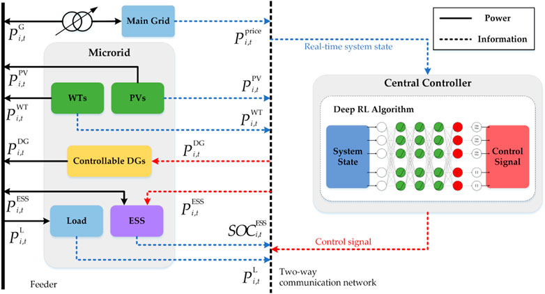
FIGURE 1. Real-time energy management framework of microgrids (MGs).

2.1.1 Modeling of DGs

Distributed generators are the main power supply unit in the MG system under study. It is assumed that the system contains a total of $D$ DGs and that the control variable of DG $i\in \mathbb{D}$ at time step $t$ is the active power output, denoted as $P_{i,t}^{DG}$. Considering the physical characteristics, the active power output of the $i$ th DG is limited to

${\mathit{P}}_{\mathit{i},\mathit{min}}^{\mathit{D}\mathit{G}}\le {\mathit{P}}_{\mathit{i},\mathit{t}}^{\mathit{D}\mathit{G}}\le {\mathit{P}}_{\mathit{i},\mathit{max}}^{\mathit{D}\mathit{G}},\mathit{i}\in \mathbb{D}=\left\{\mathbf{1,2},\cdots ,\mathit{D}\right\},$

where $P_{i,\mathit{min}}^{DG}$ and $P_{i,\mathit{max}}^{DG}$ are the minimum and maximum output power of the $i$ ^th DG, respectively. The generation cost of the $i$ ^th DG can be calculated by using a conventional quadratic function model (Zeng et al., 2019),

${\mathit{C}}_{\mathit{i},\mathit{t}}^{\mathit{D}\mathit{G}}=\left[{\mathit{a}}_{\mathit{i}}{\left({\mathit{P}}_{\mathit{i},\mathit{t}}^{\mathit{D}\mathit{G}}\right)}^{\mathbf{2}}+{\mathit{b}}_{\mathit{i}}{\mathit{P}}_{\mathit{i},\mathit{t}}^{\mathit{D}\mathit{G}}+{\mathit{c}}_{\mathit{i}}\right]\cdot ∆\mathit{t},\forall \mathit{i}\in \mathbb{D},$

where $a_i,b_i$, and $c_i$ are positive generation cost coefficients, which are determined by the physical characteristics of the DG.

2.1.2 Modeling of ESS

Energy storage systems have been widely used in recent years in power systems containing renewable energy generation. On one hand, ESSs can smooth out fluctuations in renewable energy generation, and on the other hand, they can provide power for loads when the system’s generation capacity is insufficient. The control variable of the ESS at time step $t$ is the charging or discharging power, denoted by $P_t^{ESS}$. The positive value means charging, and the negative value means discharging. During operation, an ESS cannot work in both charging and discharging states, and the operating state of an ESS is denoted by $\alpha$. $\alpha =1$ means that the ESS is charging, and $\alpha =0$ means that the ESS is discharging. The charging and discharging power constraint of an ESS at any moment is given by

$-{\mathit{P}}_{\mathit{max}}^{\mathit{E}\mathit{S}\mathit{S}}\le {\mathit{P}}_{\mathit{t}}^{\mathit{E}\mathit{S}\mathit{S}}\le {\mathit{P}}_{\mathit{max}}^{\mathit{E}\mathit{S}\mathit{S}},$

where $P_{\mathit{max}}^{ESS}$ is the maximum charging or discharging power.

The state of charge (SOC) is used as one of the indicators that prevent overcharging or overdischarging. The SOC of the ESS at time slot $t$ is denoted by ${SOC}_t$. It can be modeled as (Gibilisco et al., 2018)

${\mathit{S}\mathit{O}\mathit{C}}_{\mathit{t}}={\mathit{S}\mathit{O}\mathit{C}}_{\mathit{t}-\mathbf{1}}+\mathit{\alpha }\cdot {\mathit{P}}_{\mathit{t}}^{\mathit{E}\mathit{S}\mathit{S}}\cdot {\mathit{\eta }}_{\mathit{c}\mathit{h}}^{\mathit{E}\mathit{S}\mathit{S}}\cdot ∆\mathit{t}/{\mathit{E}}^{\mathit{E}\mathit{S}\mathit{S}}+\left(\mathbf{1}-\mathit{\alpha }\right)\cdot {\mathit{P}}_{\mathit{t}}^{\mathit{E}\mathit{S}\mathit{S}}\cdot ∆\mathit{t}/\left({\mathit{E}}^{\mathit{E}\mathit{S}\mathit{S}}\cdot {\mathit{\eta }}_{\mathit{d}\mathit{i}\mathit{s}}^{\mathit{E}\mathit{S}\mathit{S}}\right),$

where ${\eta }_{ch}^{ESS}$ and ${\eta }_{dis}^{ESS}$ are the charging and discharging efficiencies of the ESS, respectively, and $E^{ESS}$ is the capacity of the ESS. The SOC should be kept in a safe range according to its technical constraints as follows:

${\mathit{S}\mathit{O}\mathit{C}}_{\mathit{min}}\le {\mathit{S}\mathit{O}\mathit{C}}_{\mathit{t}}\le {\mathit{S}\mathit{O}\mathit{C}}_{\mathit{max}},$

where ${SOC}_{\mathit{min}}$ and ${SOC}_{\mathit{max}}$ are the minimum and maximum values of the SOC at which the ESS can operate properly, respectively.

2.1.3 Modeling of the main grid

The studied MG system is connected to the main grid through a converter and runs in a grid-connected mode. The power purchased from or sold to the main grid at each time slot is denoted by $P_t^G$. It is not possible for the MG to both buy and sell electricity from the main grid at the same time. The interaction power should satisfy the constraint

$-{\mathit{P}}_{\mathit{max}}^{\mathit{G}}\le {\mathit{P}}_{\mathit{t}}^{\mathit{G}}\le {\mathit{P}}_{\mathit{max}}^{\mathit{G}},$

where $P_{\mathit{max}}^G$ is the maximum power of the MG that can be purchased from or sold to the main grid according to the limitation of the point of common coupling (PCC), the positive value of $P_t^G$ means purchasing electricity, and the negative value means selling electricity.

Prices at which electricity is purchased or sold between the MG and the main grid are derived from the real-time electricity market. The transaction cost $C_t^G$ can be formulated as

${\mathit{C}}_{\mathit{t}}^{\mathit{G}}=\left\{\begin{array}{c}\begin{array}{cc}{\mathit{P}}_{\mathit{t}}^{\mathit{p}\mathit{r}\mathit{i}\mathit{c}\mathit{e}}\cdot {\mathit{P}}_{\mathit{t}}^{\mathit{G}}\cdot ∆\mathit{t},& {\mathit{P}}_{\mathit{t}}^{\mathit{G}}\ge \mathbf{0}\end{array},\\ \begin{array}{cc}{\mathit{\beta }}^{\mathit{G}}\cdot {\mathit{P}}_{\mathit{t}}^{\mathit{p}\mathit{r}\mathit{i}\mathit{c}\mathit{e}}\cdot {\mathit{P}}_{\mathit{t}}^{\mathit{G}}\cdot ∆\mathit{t},& {\mathit{P}}_{\mathit{t}}^{\mathit{G}}\le \mathbf{0},\end{array}\end{array}\right.$

where $P_t^{price}$ is the real-time electricity price at time slot $t$ and $0<{\beta }^G<1$ is a discount factor that means the selling price is lower than the purchasing price.

2.1.4 Modeling of uncertainty

In the real-time energy management problem of MGs, both the load and the generation of RESs are subjected to real-time uncertainty. The power output of the wind turbine and PV can be denoted as $P_t^{PV}$ and $P_t^{WT}$, respectively, and the load is denoted by $P_t^L$. Due to the randomness of these system variables, the transition between these states variables is modeled by the transition probabilities $\mathit{Pr}\left\{{state}_{t+1}|{state}_t\right\}$ and ${state}_t=\left\{P_t^{PV},P_t^{WT},P_t^L\right\}$. However, the explicit model of transition probability cannot be obtained because of uncertainty. In the existing model-based research work, wind speed and light or their errors are usually assumed to follow known probability distributions (Liang and Tang, 2020; Khosravi et al., 2022; Malik et al., 2022) and are used to model wind power and PV output to obtain renewable energy output data. However, the modeling process for these probability distribution models is complex, the parameters are difficult to identify, and a large sample of actual operational data is required, which is very time consuming (Jiang et al., 2021). Furthermore, the actual system operating data do not strictly obey these probability distribution functions, so we use the historical data of real power systems to learn the transition probability. Details about the used historical data are presented in Section 3.

2.1.5 Constraint of power balance

The power balance constraint should be considered when the MG works in both the grid-connected mode and islanded mode. The power balance constraint of the system is described by

${\sum }_{\mathit{i}}^{\mathit{D}}{\mathit{P}}_{\mathit{i},\mathit{t}}^{\mathit{D}\mathit{G}}+{\mathit{P}}_{\mathit{t}}^{\mathit{G}}+{\mathit{P}}_{\mathit{t}}^{\mathit{P}\mathit{V}}+{\mathit{P}}_{\mathit{t}}^{\mathit{W}\mathit{T}}={\mathit{P}}_{\mathit{t}}^{\mathit{L}}+{\mathit{P}}_{\mathit{t}}^{\mathit{E}\mathit{S}\mathit{S}},\mathit{t}=\mathbf{1,2},\cdots ,\mathit{T},$

where variables on the left side of the equal sign represent the power suppliers and variables on the right side of the equal sign represent the power demand side.

2.2 Problem formulation

The most significant challenge in modeling the real-time energy management problem of MGs is the variety of uncertain variables in the system. An MDP model that takes into account the uncertainty is formulated in this section to solve the real-time energy management problem for MGs. The objective is to reduce the cumulative daily operating costs of the system. The MDP is solved using the proposed DRL method present in Section 2.3. The MDP model is represented by a 5-tuple $\left(\mathcal{S},\mathcal{A},P_{s{s}^{\prime }}^a,r,\gamma \right)$. The state variable, action variable, and reward function of the system are reasonably designed in the model.

2.2.1 System state

The state of the system at any time step $t$ can be expressed as (Ji et al., 2019)

${\mathit{s}}_{\mathit{t}}=\left({\mathit{P}}_{\mathit{t}-\mathbf{23}}^{\mathit{L}},\cdots ,{\mathit{P}}_{\mathit{t}}^{\mathit{L}},{\mathit{P}}_{\mathit{t}-\mathbf{23}}^{\mathit{W}\mathit{T}},\cdots ,{\mathit{P}}_{\mathit{t}}^{\mathit{W}\mathit{T}},{\mathit{P}}_{\mathit{t}-\mathbf{23}}^{\mathit{P}\mathit{V}},\cdots ,{\mathit{P}}_{\mathit{t}}^{\mathit{P}\mathit{V}},{\mathit{P}}_{\mathit{t}-\mathbf{23}}^{\mathit{p}\mathit{r}\mathit{i}\mathit{c}\mathit{e}},\cdots ,{\mathit{P}}_{\mathit{t}}^{\mathit{p}\mathit{r}\mathit{i}\mathit{c}\mathit{e}},{\mathit{S}\mathit{O}\mathit{C}}_{\mathit{t}},\mathit{t}\right),{\mathit{s}}_{\mathit{t}}\in \mathcal{S}.$

The defined system state consists of the latest 24 h history information, $P_{t-23}^L,\cdots ,P_t^L$ are the latest 24 h loads, $P_{t-23}^{WT},\cdots ,P_t^{WT},P_{t-23}^{PV},\cdots ,P_t^{PV}$ are the latest 24 h power output of wind and photovoltaic, respectively, $P_{t-23}^{price},\cdots ,P_t^{price}$ are the latest 24 h electricity prices, and $\mathcal{S}$ is the set of all possible states.

The formulation of the system state considers historical information, which can improve the reliability of the learning method to some degree but increase the dimensionality of the state variables and the computational complexity. The problem is exacerbated when the composition and size of the system grow. To reduce the computational complexity, the representation of the system state can be simplified as

${\mathit{s}}_{\mathit{t}}=\left({\mathit{P}}_{\mathit{t}}^{\mathit{L}},{\mathit{P}}_{\mathit{t}}^{\mathit{W}\mathit{T}},{\mathit{P}}_{\mathit{t}}^{\mathit{P}\mathit{V}},{\mathit{P}}_{\mathit{t}}^{\mathit{p}\mathit{r}\mathit{i}\mathit{c}\mathit{e}},{\mathit{S}\mathit{O}\mathit{C}}_{\mathit{t}},\mathit{t}\right),{\mathit{s}}_{\mathit{t}}\in \mathcal{S},\forall \mathit{t}.$

2.2.2 Action

The control variables consist of the active power of the DG as well as the charging and discharging power of the ESS. The power interacting with the main grid can be calculated according to the balance constraint after obtaining the power of DGs and ESSs. The action $a_t$ to be performed by the system at each time step $t$ according to the state $s_t$ is defined as

${\mathit{a}}_{\mathit{t}}=\left({{\mathit{P}}_{\mathbf{1},\mathit{t}}^{\mathit{D}\mathit{G}},\cdots ,\mathit{P}}_{\mathit{D},\mathit{t}}^{\mathit{D}\mathit{G}},{\mathit{P}}_{\mathit{t}}^{\mathit{E}\mathit{S}\mathit{S}}\right),{\mathit{a}}_{\mathit{t}}\in \mathcal{A}\left({\mathit{s}}_{\mathit{t}}\right),\forall \mathit{t},$

where $\mathcal{A}\left(s_t\right)$ is the set of all possible actions when the system is in state $s_t$.

According to the presentation of action, the action set $\mathcal{A}\left({\mathit{s}}_t\right)$ can be divided into two parts:

$\mathcal{A}\left({\mathit{s}}_{\mathit{t}}\right)={\left({\mathcal{A}}^{\mathit{D}\mathit{G}}\left({\mathit{s}}_{\mathit{t}}\right)\right)}^{\mathit{D}}\times {\mathcal{A}}^{\mathit{E}\mathit{S}\mathit{S}}\left({\mathit{s}}_{\mathit{t}}\right),$

where ${\left({\mathcal{A}}^{DG}\left(s_t\right)\right)}^D$ is the action set of $D$ DGs and ${\mathcal{A}}^{ESS}\left(s_t\right)$ is the action set of the ESS.

In a learning-based approach, the processing of the action space can be divided in two ways. One is to discretize the action space, where the agent selects actions in a limited discrete action space based on the system state, and the other is to select in a continuous action space based on a deterministic policy or a stochastic policy. The size of the discrete action space will affect the accuracy of action selection, so the continuous action space is used in this work.

2.2.3 Reward and objective

The reward at each time step $t$ is the negative operating cost of the MG system and is defined by

${\mathit{r}}_{\mathit{t}}\left({\mathit{s}}_{\mathit{t}},{\mathit{a}}_{\mathit{t}}\right)=-\left({\mathit{C}}_{\mathit{t}}^{\mathit{G}}+{{\displaystyle \sum }}_{\mathit{i}}^{\mathit{D}}{\mathit{C}}_{\mathit{i},\mathit{t}}^{\mathit{D}\mathit{G}}+{\mathit{C}}_{\mathit{t}}^{\mathit{P}\mathit{e}\mathit{n}}\right),$

where $C_t^{Pen}=\sigma \cdot V_t^{Pen}$ is the penalty term, $\sigma$ is the penalty factor, and $V_t^{Pen}$ is the penalty value. During the training process, a large penalty value is set in the reward function to guide the policy network to learn under the constraints when the constraints of the system are not satisfied. $V_t^{Pen}$ is expressed in the following form:

${\mathit{V}}_{\mathit{t}}^{\mathit{P}\mathit{e}\mathit{n}}=\mathbf{max}\left(\mathbf{0},{{\mathit{S}\mathit{O}\mathit{C}}_{\mathit{t}}-\mathit{S}\mathit{O}\mathit{C}}_{\mathit{max}}\right)+\mathbf{max}\left(\mathbf{0},{\mathit{S}\mathit{O}\mathit{C}}_{\mathit{min}}-{\mathit{S}\mathit{O}\mathit{C}}_{\mathit{t}}\right)+\mathbf{max}\left(\mathbf{0},{\mathit{P}}_{\mathit{t}}^{\mathit{G}}-{\mathit{P}}_{\mathit{max}}^{\mathit{G}}\right)+\mathbf{max}\left(\mathbf{0},-{\mathit{P}}_{\mathit{max}}^{\mathit{G}}-{\mathit{P}}_{\mathit{t}}^{\mathit{G}}\right).$

The objective of the MDP is to maximize the cumulative reward within a limited scheduling time, which means to minimize the total operating cost of the system over a period of time. We define the control strategy that can maximize the cumulative reward of the MDP as ${\pi }^{*}$, and then, the objective can be expressed as

${\mathit{V}}^{{\mathit{\pi }}^{*}}\left({\mathit{s}}_{\mathbf{0}}\right)=\underset{\mathit{\pi }\in \mathit{\Pi }}{\mathbf{max}}{\mathbb{E}}_{\mathit{\pi }}\left[{\sum }_{\mathit{t}=\mathbf{0}}^{\mathit{T}}{\mathit{\gamma }}^{\mathit{t}}\cdot {\mathit{r}}_{\mathit{t}+\mathbf{1}}\left|{\mathit{s}}_{\mathbf{0}}\right.\right],$

where $V^{{\pi }^{*}}$ is the expected optimal maximum cumulative reward, ${\mathit{s}}_0$ is the initial state of the MG system, $\mathrm{\Pi }$ is the set of all possible policies, ${\mathbb{E}}_{\pi }\left[\bullet \right]$ denotes the expected value of the policy $\pi$, and $0<\gamma <1$ is a discount factor that determines the importance of future rewards.

2.2.4 Transition probabilities

In the MDP model, the system executing the action $a_t$ at state $s_t$ will move to state $s_{t+1}$ according to the system transition probability model:

${\mathit{P}}_{\mathit{s}{\mathit{s}}^{\prime }}^{\mathit{a}}=\mathit{T}\mathit{r}\left\{{\mathit{s}}^{\prime }={\mathit{s}}_{\mathit{t}+\mathbf{1}}|\mathit{s}={\mathit{s}}_{\mathit{t}},\mathit{a}={\mathit{a}}_{\mathit{t}}\right\}.$

The transition probability model is presented in Figure 2. In an MG system with a known transition model, the transition probability $P_{s{s}^{\prime }}^a$ is determined, which means that when the system is in state $s_t$, it can be transferred to a determined state $s_{t+1}$ after executing action $a_t$ according to the control strategy. The transition probability is affected by the current state and the action chosen by the control strategy. However, the system state variables of load, electricity price, and renewable energy generation are all uncertain in real time, and it is not attainable to determine the state information for the next moment based only on the current state and decision action. The SOC of the ESS can be state transferred according to the model of ESS.

FIGURE 2

FIGURE 2. Transition probability model of MDP.

The transfer model of the system can be obtained through short-term prediction or Monte Carlo simulation (Ji et al., 2019). Short-term prediction methods suffer from prediction errors, and the MC simulation method requires a large amount of sampling (Malik et al., 2022). The approach used in our work does not require short-term forecasting or sampling simulations but rather learning from real power system data to simulate the interaction with the real power system. Learning directly from historical state data of real power systems does not require the construction of prediction models, thus allowing prediction errors due to models and parameters to be avoided. For renewable energy output, training uses historical power data and does not require large amounts of meteorological data as samples, or the construction of generation models based on meteorological data.

2.3 Proposed deep reinforcement learning method

The formulated MDP model has continuous and high-dimensional actions. Due to the curse of dimensionality, it is difficult for the traditional RL algorithms to handle such problems. This section proposes a gradient-based policy learning approach for solving the MDP. A DNN-based deterministic policy is designed to approximate the optimal policy ${\pi }^{*}\left(a_t\left|s_t\right.\right)$. The neural network-based policy can generate deterministic continuous actions based on the observation of the system state. To optimize the policy, the DDPG algorithm is adopted to train the scheduling policy network. The experience-replay technology is used to train the network to ensure the stability and convergence of the network.

2.3.1 Reinforcement learning model

The optimization problem is reformulated into the standard reinforcement learning framework (Sutton and Barto, 1998). The objective in the RL framework is shown as follows:

${\mathit{V}}^{{\mathit{\pi }}^{*}}\left({\mathit{s}}_{\mathit{t}}\right)=\underset{{\mathit{a}}_{\mathit{t}}\in \mathcal{A}\left({\mathit{s}}_{\mathit{t}}\right)}{\mathbf{max}}{\mathit{Q}}^{{\mathit{\pi }}^{*}}\left({\mathit{s}}_{\mathit{t}},{\mathit{a}}_{\mathit{t}}\right),$

where $Q^{{\pi }^{*}}$ is the optimal action-value function.

The action-value function $Q^{\pi }\left(s_t,a_t\right)$ describes the expected rewards for taking action $a_t$ and then following policy $\pi$ in state $s_t$ (Lillicrap et al., 2015). It is denoted by

${\mathit{Q}}^{\mathit{\pi }}\left({\mathit{s}}_{\mathit{t}},{\mathit{a}}_{\mathit{t}}\right)={\mathbb{E}}_{{\mathit{r}}_{\mathit{i}>\mathit{t}},{\mathit{s}}_{\mathit{i}>\mathit{t}}\sim {\mathit{P}}_{\mathit{s}{\mathit{s}}^{\prime }}^{\mathit{a}},{\mathit{a}}_{\mathit{i}>\mathit{t}}\sim \mathit{\pi }}\left[{\mathit{r}}_{\mathit{t}}\left|{\mathit{s}}_{\mathit{t}},{\mathit{a}}_{\mathit{t}}\right.\right].$

The optimal action-value function $Q^{{\pi }^{*}}$ satisfies a recursive relationship, also known as the Bellman optimality equation. The optimal action-value function can be obtained by solving the Bellman equation, and then, the optimal policy ${\pi }^{*}$ and the optimal actions can be obtained by

${\mathit{Q}}^{{\mathit{\pi }}^{*}}\left({\mathit{s}}_{\mathit{t}},{\mathit{a}}_{\mathit{t}}\right)={\mathbb{E}}_{{\mathit{\pi }}^{*}}\left[{\mathit{r}}_{\mathit{t}}+\mathit{\gamma }\cdot \underset{{\mathit{a}}_{\mathit{t}+\mathbf{1}}\in \mathcal{A}\left({\mathit{s}}_{\mathit{t}}\right)}{\mathbf{max}}{\mathit{Q}}^{{\mathit{\pi }}^{*}}\left({\mathit{s}}_{\mathit{t}+\mathbf{1}},{\mathit{a}}_{\mathit{t}+\mathbf{1}}\right)\right],$

${\mathit{\pi }}^{*}\left({\mathit{s}}_{\mathit{t}}\right)=\underset{{\mathit{a}}_{\mathit{t}}\in \mathcal{A}\left({\mathit{s}}_{\mathit{t}}\right)}{\mathbf{argmax}}{\mathit{Q}}^{{\mathit{\pi }}^{*}}\left({\mathit{s}}_{\mathit{t}},{\mathit{a}}_{\mathit{t}}\right).$

The Bellman equation will be difficult to solve when faced with complex problems. To address this problem, value-based methods, such as Q-learning (Watkins and Dayan, 1992) and DQN (Mnih et al., 2015), use a look-up table or DNN to estimate the optimal action-value function $Q^{{\pi }^{*}}$ and update it iteratively. The approximation function is usually described in the form of a function $Q\left(s,a|{\theta }^Q\right)$ with respect to parameter ${\theta }^Q$, and the parameters are optimized with the objective of minimizing the loss function Loss based on the temporal-difference (TD) theory.

$\mathit{L}\left({\mathit{\theta }}^{\mathit{Q}}\right)={\mathbb{E}}_{{\mathit{s}}_{\mathit{t}}\sim {\mathit{\rho }}^{\mathit{\beta }},{\mathit{a}}_{\mathit{t}}\sim \mathit{\beta }}\left[{\left({\mathit{y}}_{\mathit{t}}-\mathit{Q}\left({\mathit{s}}_{\mathit{t}},{\mathit{a}}_{\mathit{t}}|{\mathit{\theta }}^{\mathit{Q}}\right)\right)}^{\mathbf{2}}\right],$

where $B$ is the batch size of the samples sampled from the replay buffer and $y_t$ is the target value.

${\mathit{y}}_{\mathit{t}}={\mathit{r}}_{\mathit{t}}\left({\mathit{s}}_{\mathit{t}},{\mathit{a}}_{\mathit{t}}\right)+\mathit{\gamma }\cdot \mathit{Q}\left({\mathit{s}}_{\mathit{t}+\mathbf{1}},\mathit{\mu }\left({\mathit{s}}_{\mathit{t}+\mathbf{1}}\right)|{\mathit{\theta }}^{\mathit{Q}}\right).$

Reinforcement learning that uses an approximation function to estimate the value function is known as the value-based RL method. However, it has some disadvantages in practical applications, especially when dealing with problems with continuous action spaces where a good scheduling strategy cannot be obtained. Therefore, we use policy-based reinforcement learning methods (Sutton et al., 2000), which can directly approximate the policy and optimize the policy function through the gradient ascent method until a convergent policy is obtained.

2.3.2 Policy-based reinforcement learning and deep deterministic policy gradient method

The deep deterministic policy gradient (Silver et al., 2014) algorithm is introduced to solve the complex coordinate EV charging and voltage control problem with high-dimensional and continuous action spaces by only using low-dimensional observations. The DDPG algorithm is a policy-based DRL algorithm with actor–critic architecture. Both the actor and critic contain two neural networks, with the actor consisting of two DNNs with parameters ${\theta }^{\mu }$ and ${\theta }^{{\mu }^{\prime }}$ and the critic consisting of two multilayer perceptron (MLP) with parameters ${\theta }^Q$ and ${\theta }^{Q^{\prime }}$, respectively. The construction of the DDPG algorithm is shown in Figure 3. Similar to the standard reinforcement learning, the DDPG has a learning agent that interacts with a distribution network environment in discrete timesteps. The input of the DDPG agent is the system state $s_t$ at time step $t$, and the output is action $a_t$. We assume the studied DN environment is fully observed. To ensure the independence between samples when using neural networks, the DDPG uses experience replay technology to ensure independence between the samples used for target value updating. After each interaction of the agent with the environment, we can obtain a sample containing $s_t$, $a_t$, $r_t$, and $s_{t+1}$ and store this sample in the replay buffer. The agent continues to interact with the environment until the set condition is met, and then, $B$ samples are randomly sampled from the replay buffer to minimize the loss of the critic network and to calculate the gradient of the actor network to softly update the parameters of the critic and actor networks.

FIGURE 3

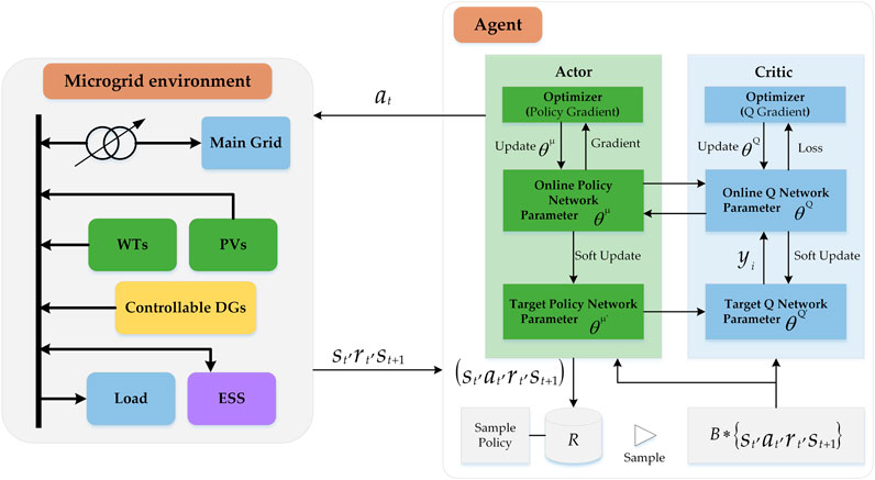
FIGURE 3. Structure of the proposed DDPG algorithm.

The DDPG algorithm combines the success of the actor–critic approach and DQN (Mnih et al., 2015) using dual networks on top of the deterministic policy gradient (DPG) algorithm (Silver et al., 2014). The DPG algorithm is based on the actor–critic structure, which consists of an actor and a critic. The critic $Q\left(s,a\right)$ is learned using the Bellman equation as in Q-learning. According to the loss function, the update rule for the parameters of the critic is given by (Lillicrap et al., 2015).

$\mathit{L}\left({\mathit{\theta }}^{\mathit{Q}}\right)=\frac{\mathbf{1}}{\mathit{B}}{\sum }_{\mathit{i}}{\left({\mathit{y}}_{\mathit{i}}-\mathit{Q}\left({\mathit{s}}_{\mathit{i}},{\mathit{a}}_{\mathit{i}}|{\mathit{\theta }}^{\mathit{Q}}\right)\right)}^{\mathbf{2}}.$

The actor is a parameterized actor function $\mu \left(s|{\theta }^{\mu }\right)$ that specifies the current policy by deterministically mapping states to actions. The actor value networks are updated according to policy gradients by using the gradient ascent method and the sampled sequence of decisions, and the chain rule is used to the expected return $J$ from the start distribution to update the actor. The update rule for the parameters of the actor is given by

${\nabla }_{{\mathit{\theta }}^{\mathit{\mu }}}\mathit{J}\approx {\mathbb{E}}_{{\mathit{s}}_{\mathit{t}}\sim {\mathit{\rho }}^{\mathit{\beta }}}\left[{\nabla }_{{\mathit{\theta }}^{\mathit{\mu }}}\mathit{Q}\left(\mathit{s},\mathit{a}|{\mathit{\theta }}^{\mathit{Q}}\right){|}_{\mathit{s}={\mathit{s}}_{\mathit{t}},\mathit{a}=\mathit{\mu }\left({\mathit{s}}_{\mathit{t}}|{\mathit{\theta }}^{\mathit{\mu }}\right)}\right],$

$={\mathbb{E}}_{{\mathit{s}}_{\mathit{t}}\sim {\mathit{\rho }}^{\mathit{\beta }}}\left[{\nabla }_{\mathit{a}}\mathit{Q}\left(\mathit{s},\mathit{a}|{\mathit{\theta }}^{\mathit{Q}}\right){|}_{\mathit{s}={\mathit{s}}_{\mathit{t}},\mathit{a}=\mathit{\mu }\left({\mathit{s}}_{\mathit{t}}\right)}{\nabla }_{{\mathit{\theta }}_{\mathit{\mu }}}\mathit{\mu }\left(\mathit{s}|{\mathit{\theta }}^{\mathit{\mu }}\right){|}_{\mathit{s}={\mathit{s}}_{\mathit{t}}}\right],$

$\approx \frac{\mathbf{1}}{\mathit{B}}{\displaystyle \sum }_{\mathit{i}}{\nabla }_{\mathit{a}}\mathit{Q}\left(\mathit{s},\mathit{a}\left|{\mathit{\theta }}^{\mathit{Q}}\right.\right){|}_{\mathit{s}={\mathit{s}}_{\mathit{i}},\mathit{a}=\mathit{\mu }\left({\mathit{s}}_{\mathit{i}}\right)}\cdot {\nabla }_{{\mathit{\theta }}^{\mathit{\mu }}}\mathit{\mu }\left(\mathit{s}|{\mathit{\theta }}^{\mathit{\mu }}\right){|}_{{\mathit{s}}_{\mathit{i}}},$

where $J$ is the expected return from the start distribution, $\mu$ is the deterministic target policy, $\theta$ is the parameter of the function approximator, $\rho$ is the discounted state visitation distribution for policy, $\beta$ is a different stochastic behavior policy, and $s_i$ is the state of the $i\mathrm{t}\mathrm{h}$ sample in the small batch of samples sampled from the replay buffer.

The main challenge of learning in continuous action spaces is exploration. DDPG constructs an exploration policy ${\mu }^{\prime }$ by adding noise samples from a noise process $\mathcal{N}$ to the actor policy. The noise process $\mathcal{N}$ can be chosen according to the characteristics of the environment under study. Because the energy management problem of the MG is not the same as traditional physical control problems with inertia, the noise process is not used in our practical implementation to increase the exploration of the action space.

${\mathit{a}}_{\mathit{t}}={\mathit{\mu }}^{\prime }\left({\mathit{s}}_{\mathit{t}}\right)=\mathit{\mu }\left({\mathit{s}}_{\mathit{t}}|{\mathit{\theta }}^{\mathit{\mu }}\right)+{\mathcal{N}}_{\mathit{t}}.$

2.3.3 Design of the deep neural network

Traditional RL methods use tables or polynomial functions to provide an approximation to the optimal action-value function. These forms are relatively simple to understand, but they cannot be effectively learned and trained when faced with high-dimensional complex problems. To overcome these challenges, we design a DNN to approximate the optimal policy. The designed architecture of the policy network is presented in Figure 4.

FIGURE 4

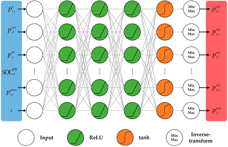
FIGURE 4. Architecture of the designed policy network.

The status information on the system’s renewable energy output $P_t^{WT},P_t^{PV}$, load demand $P_t^L$, real-time LMP price $P_t^{price}$, and SOC of the ESS ${SOC}_t$ is fed into the network, and the output is a defined continuous action vector. To ensure the stability and convergence of the learning process, all input state data are normalized according to their respective maximum–minimum values. An RNN can be used as a policy network when the state variables contain information from the past $T$ time periods. In the model we build, the state variables only contain information from the current moment to reduce the dimensionality of the state space, so we choose a DNN as the policy network to extract the feature information of the system state variables. To alleviate the problem of vanishing gradient or exploding gradient, a rectified linear unit (ReLU) is used as the activation function of each neuron in the hidden layer. The output layer uses the tanh activation function to directly output the action vector $a_t$ of the system in the current state $s_t$. The final layer of the network uses tanh as the activation function and outputs continuous values in the range [−1, 1]. The inverse-transform block in the figure behind the output layer represents the limit on the range of output continuous actions, corresponding to the constraints on DGs and the ESS in Section 2.

The details of the architecture of the policy network of the proposed DDPG structure are provided in Table 1. The designed policy network has five layers, of which the first and fifth layers are the input and output layers, respectively, and the remaining three layers are the hidden layers. The dimensionality of the input layer corresponds to the dimensionality of the system state variables $N^S$, and the dimensionality of the output layer corresponds to the dimensionality of the system action variables $N^A$. As the dimension of the input states is small, we set the depth of the hidden layer to 3 in order to converge quickly and avoid gradient disappearance, and if the number of dimensions of the input states increases, the number of layers of the hidden layer can be increased appropriately. The width of the hidden layers is related to the dimensionality of the states and is set to $2^{N^S}$ to learn the features of the states. However, the width of the network should be too large to prevent overfitting when faced with higher-dimensional state inputs.

TABLE 1

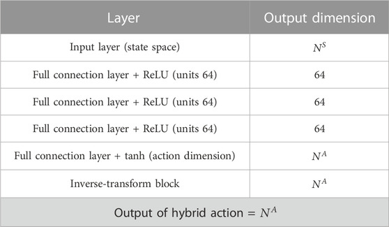
TABLE 1. Policy network structure.

2.3.4 Offline training and online running

The scheduling process of the MG can be summarized as the offline training and online scheduling process presented in Figure 5. The agent is trained in a centralized mode using historical system data and then runs in an online mode. The parameters (weights and biases) of the initial policy of the agent are random, and the policy network cannot output the optimal action. Therefore, the policy network of the agent needs to be trained in an offline mode using historical environmental data before it can practically operate. The parameters of the DNN are updated through an iterative interaction with the environment and the accumulation of experience. With this approach, the agent can gradually optimize the network parameters to more accurately approach the optimal collaborative strategy. The pseudocode for the training procedure of the DDPG approach is presented in Algorithm 1. In Algorithm 1, all network parameters (weights and biases) of the DDPG are initialized before starting training. At the beginning of each episode, the environment is reset to obtain the initial state of the system. Then, the policy network under the current parameters is used to interact with the environment for $T$ time steps. During the interaction, the immediate reward, the observed state at the next moment, the current state, and the action are composed to be one sample, and this sample is stored in the replay buffer. Then, a random batch of samples from the replay buffer is used to update the parameters of the actor and critic networks of the DDPG according to the conditions.

FIGURE 5

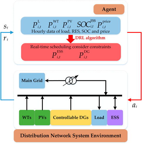
FIGURE 5. Schematic of the framework for offline training and online operation.

Algorithm 1. DDPG-based learning algorithm.

1: Initialize weights ${\theta }^Q$ and ${\theta }^{\mu }$ of critic network $Q\left(s,a|{\theta }^Q\right)$ and actor network $\mu \left(s|{\theta }^{\mu }\right)$

2: Initialize weights ${\theta }^{Q^{\prime }}\leftarrow {\theta }^Q$ and ${\theta }^{{\mu }^{\prime }}\leftarrow {\theta }^{\mu }$ of target network $Q^{\prime }$ and ${\mu }^{\prime }$

3: Initialize experience replay buffer $R$

4: for $episode$ = 1, 2, … , $M$ do

5: Receive initial observation state $s_1$

6: for $t$ = 1, 2, … , $T$ do

7: Choose $a_t=\mu \left(s_t|{\theta }^{\mu }\right)$

8: Observe reward $r_t$ and the next state $s_{t+1}$

9: Store transition $\left(s_t,a_t,r_1,s_{t+1}\right)$ in $R$

10: Sample a random minibatch of $B$ transitions $\left(s_i,a_i,r_i,s_{i+1}\right)$ from $R$

11: Set ${\mathit{y}}_{\mathit{i}}={\mathit{r}}_{\mathit{i}}+\mathit{\gamma }\cdot {\mathit{Q}}^{\prime }\left({\mathit{s}}_{\mathit{i}+\mathbf{1}},{\mathit{\mu }}^{\prime }\left({\mathit{s}}_{\mathit{i}+\mathbf{1}}|{\mathit{\theta }}^{{\mathit{\mu }}^{\prime }}\right)|{\mathit{\theta }}^{{\mathit{Q}}^{\prime }}\right)$

12: Update critic network parameters by minimizing the loss: $\mathit{L}=\frac{\mathbf{1}}{\mathit{B}}{\sum }_{\mathit{i}}{\left({\mathit{y}}_{\mathit{i}}-\mathit{Q}\left({\mathit{s}}_{\mathit{i}},{\mathit{a}}_{\mathit{i}}|{\mathit{\theta }}^{\mathit{Q}}\right)\right)}^{\mathbf{2}}$

13: Update the actor policy using the sampled policy gradient: ${\nabla }_{{\mathit{\theta }}^{\mathit{\mu }}}\mathit{J}\approx \frac{\mathbf{1}}{\mathit{B}}{\displaystyle \sum }_{\mathit{i}}{\nabla }_{\mathit{a}}\mathit{Q}\left(\mathit{s},\mathit{a}\left|{\mathit{\theta }}^{\mathit{Q}}\right.\right){|}_{\mathit{s}={\mathit{s}}_{\mathit{i}},\mathit{a}=\mathit{\mu }\left({\mathit{s}}_{\mathit{i}}\right)}\cdot {\nabla }_{{\mathit{\theta }}^{\mathit{\mu }}}\mathit{\mu }\left(\mathit{s}|{\mathit{\theta }}^{\mathit{\mu }}\right){|}_{{\mathit{s}}_{\mathit{i}}}$

14: Softly update the target networks using the updated critic and actor network parameters: ${\mathit{\theta }}^{{\mathit{Q}}^{\prime }}\leftarrow \mathit{\tau }{\mathit{\theta }}^{\mathit{Q}}+\left(\mathbf{1}-\mathit{\tau }\right){\mathit{\theta }}^{\mathit{Q}}$ and ${\mathit{\theta }}^{{\mathit{\mu }}^{\prime }}\leftarrow \mathit{\tau }{\mathit{\theta }}^{\mathit{\mu }}+\left(\mathbf{1}-\mathit{\tau }\right){\mathit{\theta }}^{\mathit{\mu }}$

15: end for

16: end for

3 Results and discussion

In this section, we present the details of simulation experiments to test the proposed method and prove the effectiveness of the method through the analysis of the simulation results. The simulations are trained and tested using a personal computer with an NVIDIA RTX 3070 GPU and one Intel (R) Core (TM) i7-10700K CPU. The code is written in Python 3.7.8, and the reinforcement learning algorithm is implemented using the deep learning package TensorFlow 1.14.0 (Abadi et al., 2015).

3.1 The studied MG system and parameter setting

3.1.1 Description of the MG system

To reflect the effectiveness of the proposed DDPG algorithm in solving complex energy management problems considering uncertainties, an MG system with more DGs based on the European benchmark low-voltage MG system (Papathanassiou et al., 2005) is studied in this paper. The structure is presented in Figure 6. The MG system works with a central controller (CC) that can communicate with local controllers (LCs) through real-time two-way communication.

FIGURE 6

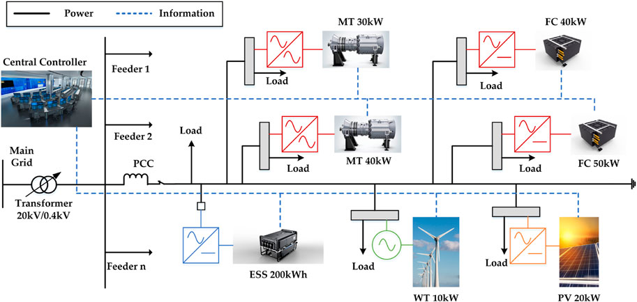
FIGURE 6. Schematic of the framework for offline training and online operation.

The simulated MG system consists of four controllable DGs ($D=4$), including two microturbines (MTs) and two fuel cells (FCs) (numbered DG1–DG4); two RESs, including a PV and a WT; a battery energy storage system; and some local loads. The operational cost function for DGs is modeled as a quadratic function in Section 2.1. The parameters of the DGs’ generation costs and the range of the power generation are given in Table 2. The capacity of the ESS is 200 kWh, and the safe range for the SOC of the ESS is [0.15, 0.98]. The max charging or discharging power of the ESS is 40 kW, and the charging and discharging rates of the ESS are 0.98 and 0.95, respectively. The capacity of the WT in the system is 10 kW and the capacity of the PV is 20 kW. The maximum power of the MG interacting with the main grid is set at 120 kW, and when the MG sells power to the main grid, the discount factor of the selling price is ${\beta }^G=0.9$. The sale price is lower than the purchase price, which helps the system to prioritize the use of local generators to meet local load demand and can reduce the negative impacts of the RES on the main grid (Zhang et al., 2015; Li et al., 2016). We divide the day into $T=24$ intervals of 1 hour each, $∆t=1\mathrm{h}$.

TABLE 2

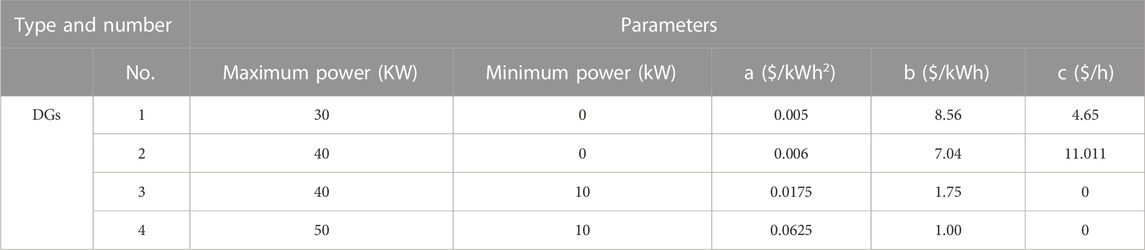
TABLE 2. Operation parameters of the components in the MG system.

3.1.2 Design of simulation experiments

Two experiments are designed to evaluate the DRL method proposed in this paper. The first experiment is to validate the responsiveness of the approach proposed in this paper to the ESS in a relatively deterministic scenario. In this scenario, the initial SOC of the ESS is set to different values; the load demand, tariff, and RES generation in the system are known. To fully demonstrate the applicability of the proposed approach, the convergence of the algorithm and the operating cost of the system are compared for different ESS parameters. The second experiment is performed to verify the practical operational performance of the approach proposed in this paper in coping with system uncertainties in a fully stochastic scenario. In this scenario, data generated by the real power system is used to simulate the state transfer process of the central controller interacting with the MG system.

Real power system data from the California Independent System Operator (CAISO) (OASIS California ISO, 2020) are used to train and test the effectiveness of the proposed approach. Data for 2019 and 2020 were downloaded as the training set and the test set, respectively. To make the range of values for the load, RES output, and electricity prices meet the requirements of the MG system under study, the downloaded raw data need to be processed. The downloaded data were first normalized and then multiplied by a set range of values to satisfy the requirements of the MG system.

3.1.3 Setting of parameters

In both simulation experiments, the designed policy network contains three hidden layers of fully connected form, each containing 64 neurons with ReLU as the activation function. tanh is chosen as the activation function of the output layer to output continuous control signals. The output control signal has a value range of [−1, 1], and we add the inverse-transform blocks after the output layer to obtain control signals in the normal value range. All the weights of the policy network are initialized to a Gaussian distribution with a bias of 0.03 and a mean of 0. The critic network contains two fully connected layers, each containing 64 neurons with ReLU as the activation function, and a linear activation function for the output layer of the network. All the weights of the critic network are initialized to a Gaussian distribution with a bias of 0.1 and a mean of 0.

The parameters considering the algorithm are given in Table 3. The number of training episodes is set to $M=3000$, which is related to the convergence rate of the algorithm, meaning that it is related to the learning rate of the actor and critic networks. The smaller learning rate of the actor is to learn better strategies and ensure the convergence of Algorithm 1. A larger learning rate for the critic than for the actor allows for faster parameter updates to the actor network. The use of a soft update for the parameters of the target networks allows for smoother parameter changes and ensures the stability of the learning process. According to the formulated MDP model, the input dimension of the policy network is 6, and the number of neurons in the hidden layers of the policy network is set to 64 = 2⁶. Setting a small number of neurons in the hidden layer can prevent overfitting. The batch size is set to $B=48$, which is smaller than the number of neurons in the hidden layers of the network to ensure that the network can fully learn the features from the batch samples. The discount factor indicates the effect of future rewards on the current action. A smaller discount factor means that the algorithm focuses more on recent decisions. However, a smaller discount factor will make the critic network unable to foresee future events. A larger discount factor means that the influence of future rewards is considered. However, a larger discount factor will make the training of the algorithm difficult. The actions output by the policy network take into account the rewards of the next $T=24$ time steps, and the discount factor is set to $\gamma =0.95$ (Sutton and Barto, 2018). The penalty factor is set to a fixed value, and the value is chosen in relation to the magnitude of the first two terms in the reward function. It should be remembered that the tuning of hyperparameters of the algorithm is not independent, and the impact of different parameters on the results and stability of the algorithm needs to be considered. The study of tuning strategies for algorithm parameters is important for improving the performance of the algorithm, but the idea of tuning the parameters of an algorithm is different when faced with different problems. How algorithm parameters affect algorithm performance and how they can be optimized, either artificially or automatically, will be the subject of future research and will not be analyzed in detail in this work.

TABLE 3

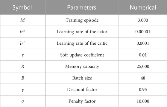
TABLE 3. Parameters of the proposed DDPG algorithm.

3.2 Experiment 1: Deterministic scenario

In the experiment with a deterministic scenario, the initial SOC of the ESS is set to different values to test the responsiveness of the proposed approach. The initial SOC of the ESS is set to 0.3, 0.5, 0.7, and 0.9.

Figure 7 gives the convergence curves of the cumulative rewards of the proposed method during training for different initial values of the SOC. As can be learned from Figure 7, the proposed approach can learn to increase the reward when the value of the initial SOC of the ESS is uncertain and the convergence curves at the four SOC values can converge to the maximum cumulative reward after 2,000 episodes. This result demonstrates that the proposed DDPG approach learns a stable policy under the deterministic environment. As can be seen from the enlarged partial graph, the algorithm has a small deviation from the values of the maximum cumulative reward at different initial values of the SOC, indicating that there is a small impact on the operating cost of the algorithm when the initial value of the SOC of the ESS is changed.

FIGURE 7

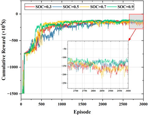
FIGURE 7. Convergence curves of the cumulative rewards of the proposed approach with different initial values of the SOC.

To further illustrate the regulating contribution of the ESS in the energy management process of the MG, we set up the ESS with different capacities and charging powers without changing other system parameters. In the simulation experiments, the initial SOC of the ESS is set to 0.9. The convergence curves of the training process of the MG system with different ESS configurations are shown in Figure 8. Based on the convergence curves shown in Figure 8, the following conclusions can be drawn: 1) the proposed approach can adapt not only to the ESS with different initial SOC values but also to the ESS with different capacities and charging power configurations; 2) the cumulative return of the system gradually decreases as the energy storage capacity increases, indicating that the configuration of the ESS with larger capacity helps to reduce the operating cost of the MG system; 3) when the capacity of the ESS is the same, the increase in the charging power also helps to reduce the operating cost of the MG system, as shown in the two curves, E200P20 and E200P40, in Figure 8. Larger capacities and charging powers usually require higher investment costs, which need to be taken into account when planning the system. However, this is not discussed in detail in our study.

FIGURE 8

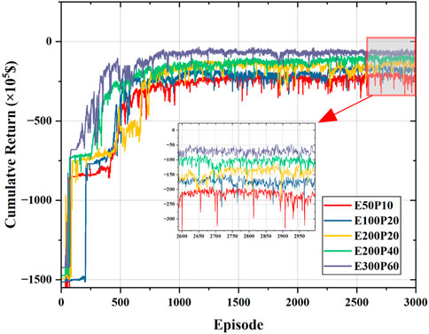
FIGURE 8. Convergence of the proposed approach with different ESS parameters.

Figure 9 presents the details of scheduling results obtained by the proposed DDPG method at an initial value of 0.45 for the SOC of the ESS. The initial SOC is set to ${SOC}_1=0.45$. According to Figure 9A, DG3 and DG4 are the main power supply units in the system because they have a lower cost of generation, while DG1 and DG2 are not the main power supply units in the system because they have a higher cost of generation. The ESS is charged and discharged according to its power storage and change in the electricity price. Based on the tariff curve in Figure 9A and the charging process of the ESS in Figure 9B, it can be seen that the ESS is able to respond to changes in tariffs. The ESS is charged at a low tariff, the SOC is subsequently increased and discharged at a high tariff, and the SOC is subsequently decreased. With the ESS, the MG is also able to respond to changes in electricity prices as it interacts with the main grid for electricity. During low-tariff hours, if the local power supply and ESS cannot meet the load demand, the MG will buy power from the main grid, and during high-tariff hours, if the power of the ESS is sufficient, the MG will sell power to the main grid to obtain some revenue. The scheduling results in Figure 9 demonstrate that the proposed DDPG approach is effective in learning an economic dispatch strategy.

FIGURE 9

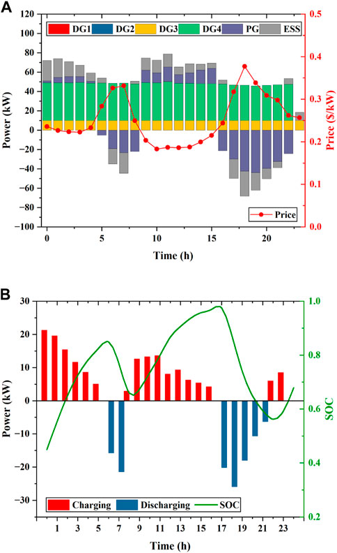
FIGURE 9. Scheduling results of the MG obtained by the proposed approach with an initial value of 0.45 for the SOC: (A) Generation schedules of DGs, ESSs, and the main grid; (B) scheduled charging or discharging power and SOC.

3.3 Experiment 2: Stochastic scenario

In the experiment with a stochastic scenario, we test the proposed algorithm using data from June and November 2020. The tested data used in the experiment are presented in Figure 10. To evaluate the performance of the proposed approach, several model-based numerical computation methods and benchmark RL solutions are used for comparison. The strategies used for comparison include random policy, greedy policy, MPC (Shi et al., 2019), MINLP policy, SAC (Haarnoja et al., 2018), PPO (Guo et al., 2022), and DQN (Ji et al., 2019) policy. The MINLP policy, in this case, represents the optimal strategy. In the MINLP policy, the system load, electricity price, and renewable energy output are assumed to be accurately predicted, and the real-time energy management problem of the MG is modeled as mixed-integer non-linear programming and solved using the commercial solver CPLEX. The random policy randomly chooses actions from a discrete action space with 11 levels of optional actions. The greedy policy aims to obtain a scheduling policy with the lowest operating cost at every timestep. The MPC policy has a sliding time window of 4 hours for the prediction time domain and 1 hour for the control time domain. The MPC policy performs one decision action based on the predicted state for the next 4 hours. The MPC policy performs this process recursively to approximate real-time control of the MG system. The DQN solution has the same discrete action space with random policy, and the output layer outputs 11⁵ discrete actions. The SAC policy, PPO policy, and DQN policy have the same policy network structure as the DDPG given in Table 1. Their hyperparameters are set with reference to the parameters given in the literature. The running time of training and testing (one step) of all algorithms is listed in Table 4. To apply the proposed method in a real power system, we perform offline training. In our study, the proposed DDPG approach took 14.21 h to train, and the time will be longer if the time interval is smaller. The parameters of the trained network are loaded during online implementation. The actual operating time during a scheduling cycle takes only a few seconds. However, traditional model-based methods take much more time to run to obtain the scheduling results. As with DDPG, both SAC and PPO are DRL algorithms based on the actor–critic structure, the difference being that SAC and PPO have fewer hyperparameters than the DDPG. However, SAC takes a longer training time to run in a multiprocessing manner, and while PPO runs in 3.3% less time than DDPG, it uses on-policy learning, which requires a large number of samples to learn. Although the DDPG has more hyperparameters that need more effort to tune, once the hyperparameters are tuned properly, the DDPG can perform better than SAC and PPO.

FIGURE 10

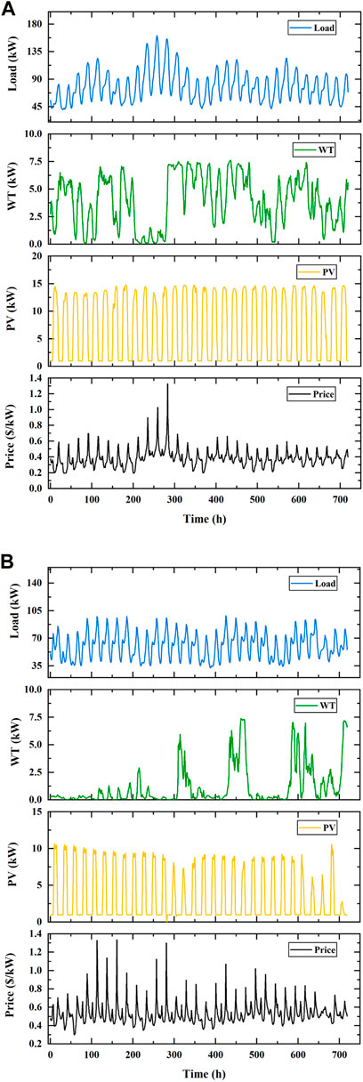
FIGURE 10. Test data used in the experiment with stochastic scenarios: (A) Data for June in the test set; (B) data for November in the test set.

TABLE 4

TABLE 4. Time consumption on training and online computation (one step) by different algorithms.

The convergence curves of the four DRL methods are presented in Figure 11. As can be seen from the figure, all four DRL methods are able to converge to stable reward values. SAC, PPO, and DDPG are policy-based DRL algorithms, and they converge faster than DQN. Among them, PPO starts to converge in less than 500 episodes because it has fewer hyperparameters, and the network parameters are updated faster; SAC converges slower than DDPG because it is trained in a multiprocessing manner; DDPG converges slower than PPO, but it obtains a higher cumulative reward than the other three DRL methods. DQN converges the slowest and has a higher error because it is a value-based DRL algorithm that updates in a more time-consuming way by selecting actions in a discrete action space.

FIGURE 11

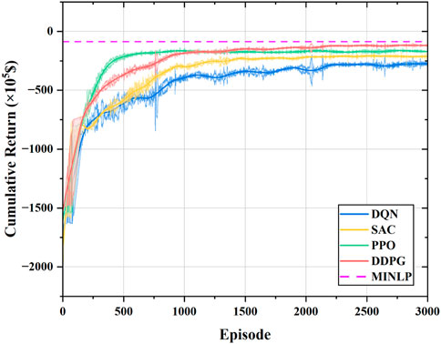
FIGURE 11. Convergence of the four DRL approaches.

The results of the cumulative daily operating cost of the proposed approach and the comparison policies on the test data are shown in Figure 12. From the results given in Figure 12, it can be seen that the random policy has the worst performance, as it has the highest cumulative operating cost, and the greedy policy has the lowest cumulative operating cost, but it does not take into account future effects. MPC has better performance than SAC and DQN, and DQN has a higher cumulative operating cost compared to SAC, which is related to the size of the action space. As can be seen from the curves in Figure 12, the DDPG has better performance than the comparison policies, obtaining lower cumulative operating costs on both the June and November test sets.

FIGURE 12

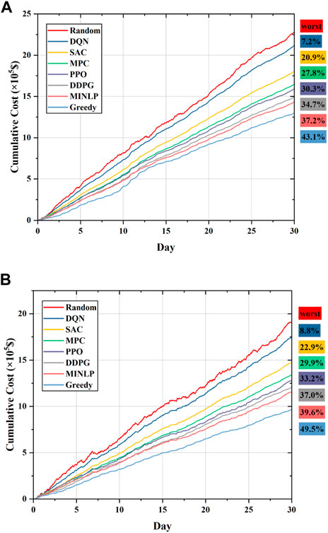
FIGURE 12. Cumulative daily operating cost over 30 consecutive days obtained by the proposed approach and the comparison methods: (A) Cumulative daily operating cost in the test set for June; (B) cumulative daily operating cost in the test set for November.

The operating costs for several policies on the test sets are given in Table 5. Based on the comparison of the numerical results, it can be seen that the greedy policy achieves the lowest cumulative running cost, but this strategy is locally optimal due to its short-sightedness. The cumulative operating costs of random, DQN, SAC, PPO, MINLP, MPC, DDPG, and greedy are $22.77K, $21.12K, $18.00K, $15.88K, $14.29K, $16.44K, $14.87K, and $12.96K for the June test set and $19.08K, $17.41K, $14.72K, $12.75K, $11.53K, $13.38K, $12.02K, and $9.64K for the November test set, respectively. The percentages of cumulative operating cost savings that can be achieved by other methods compared to the random policy can be calculated numerically and are labeled in Figure 12. Compared to the results for the cumulative operating cost of DQN, SAC, PPO, and MPC on the test set in June, the DDPG can save 29.59%, 17.39%, 6.36%, and 9.55% and can save 30.96%, 18.34%, 5.73%, and 10.16% of the cumulative operating costs on the test set in November, respectively. Compared to the results of the optimal strategy, the cumulative operating costs of the proposed DDPG approach are only 4.06% and 4.25% higher in June and November, respectively. The abovementioned analysis leads to the following conclusions: the proposed approach in this paper can operate in stochastic scenarios to obtain an economical scheduling strategy and has a more economical performance compared to the comparison policies. The numerical results show that the proposed DDPG approach is close to the optimal strategy for reducing the operating cost of MGs. Nevertheless, it is important to note that MPC, MINLP, and greedy policies all assume that the state transition probability model of the system is already known, which is often difficult to achieve in practice due to the presence of uncertainty. Only the greedy policy considers the immediate lowest cost without considering the future scenario. Although it obtains the lowest operating cost, it does not achieve optimal dispatch of the ESS.

TABLE 5

TABLE 5. Comparison of cumulative operating cost.

To further illustrate the performance of the proposed DDPG approach in reducing the operating cost of the MG system, Figure 13 presents the daily operating cost curves for the abovementioned strategies for 30 consecutive days. It can be seen from the figure that the daily running cost obtained by the DDPG policy (grey line with dots) outperforms the DQN, SAC, and MPC policies on almost all days. Compared to the PPO policy, the DDPG policy has a higher cost on some run days (marked by red circles), but according to the curves of cumulative operating cost presented in Figure 12, the DDPG policy still has lower cumulative operating cost than the PPO policy over a long period of time. The similar trend in the variation of daily running costs for several DRL strategies is attributed to the fact that we set up the same policy network structure. Furthermore, comparison of the daily operating cost curves of the DDPG policy and optimal strategies shows that the proposed DDPG policy is comparable to the optimal strategy. Based on the analysis, we can conclude that the proposed DDPG method has been proven to have a good performance in solving the real-time energy management problem of MGs.

FIGURE 13

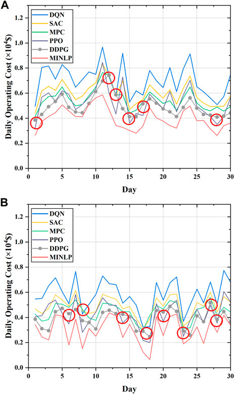
FIGURE 13. Daily operating cost over 30 consecutive days obtained by the proposed approach and the comparison methods: (A) Daily operating cost in the test set for June; (B) daily operating cost in the test set for November.

Furthermore, we calculate the error in the daily operating cost of the DRL methods and the theoretically optimal policy, and the expressed cost error $E^C$ is

${\mathit{E}}^{\mathit{C}}=\left({\mathit{C}}_{\mathit{d}}^{\mathit{D}\mathit{R}\mathit{L}}-{\mathit{C}}_{\mathit{d}}^{\mathit{O}\mathit{p}\mathit{t}}\right)/{\mathit{C}}_{\mathit{d}}^{\mathit{O}\mathit{p}\mathit{t}}\times \mathbf{100}\%,$

where $C_d^{DRL}$ denotes the operating cost of the DRL method on day d and $C_d^{Opt}$ denotes the operating cost of the optimal policy (MINLP) on day d. The results of the calculations are given in the form of a box plot in Figure 14. The results given in Figure 14 show that the proposed DDPG approach has the lowest daily operating cost error but is slightly less computationally stable than PPO.

FIGURE 14

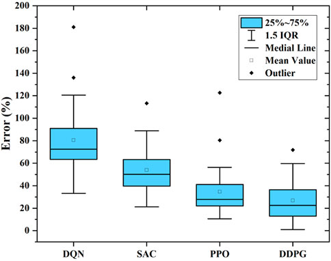
FIGURE 14. Daily operating cost error of the four DRL approaches with the optimal policy.

Figure 15 shows the results of the scheduling operation for three consecutive days. The scheduling results of the controllable units in the system are shown in Figure 15A, and the charging process of the ESS is presented in Figure 15B. The results of scheduling of the controllable units in the system are presented in Figure 15A, and the scheduled results of the ESS and the change of the SOC are shown in Figure 15B. As shown in Figure 15A, the MG will purchase a small amount of power from the main grid to meet the load demand during high-electricity price hours or sell power to the main grid to make a profit. As shown in Figure 15B, the ESS is discharged according to the power storage when the electricity price is high and is charged when the electricity price is low. It is indicated that the ESS can be effectively managed by the proposed approach in stochastic scenarios, and by adjusting the charging and discharging process of the ESS, the buffer effect of the ESS can be fully employed to reduce the operating cost of the system.

FIGURE 15

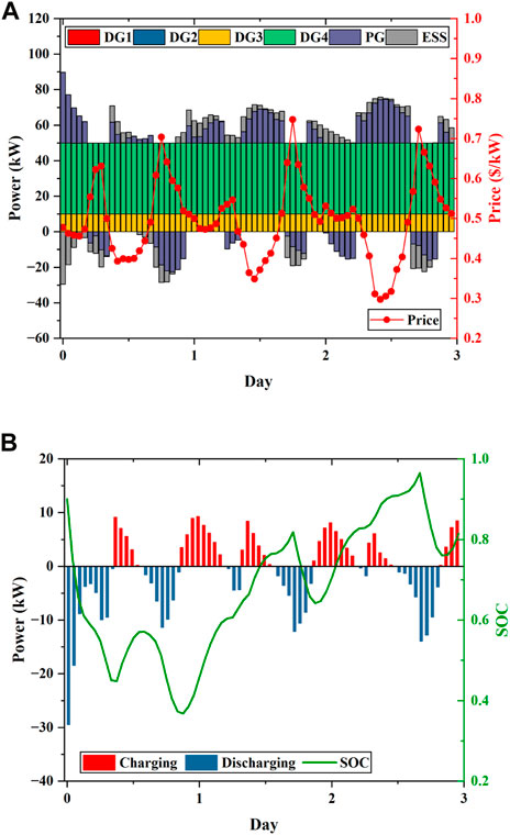
FIGURE 15. Scheduling results of the MG over three consecutive days in the test set: (A) Generation schedules of DGs, ESSs, and the main grid; (B) scheduled charging or discharging power and SOC of the ESS.

To further demonstrate the efficacy of the proposed DRL approach in addressing complex decision problems, we design a more intricate MG system. We integrate a PV, a WT, and an ESS into the current system, thereby increasing the level of uncertainty. The PV and WT have capacities of 8 kW and 15 kW, respectively. The capacity of the newly added ESS is 200 kWh, with a maximum charge and discharge power rating of 50 kW. In light of the new system structure, the number of state variables is increased by three dimensions and the number of action variables by one dimension in the new system model. While the increase in dimensionality is not significant, traditional model-based approaches would require the development of new models for the WT and PV and modifications to the algorithms. For DRL approaches with discrete action spaces, the rise in the number of action dimensions would increase the size of the action space, leading to the problem of dimensional disaster. In contrast, our approach necessitates only the minor adjustments, such as constructing a new state space for training or modifying the reward function, if necessary.

The proposed DRL method is trained offline using the algorithm parameters outlined in Section 3.1.3, and the online operation results are presented in Figure 16. Figure 16A displays the dispatch results of all controllable units and the main grid in the system, while Figure 16B and Figure 16C show the charging and discharging status and SOC variations of two ESSs, respectively. As demonstrated in Figure 16A, with the increase in energy storage units in the system, the MG tends to purchase more electricity from the main grid and store it in the ESS during low electricity prices and discharge the ESS to meet the load demand during high electricity prices, or even sell the low-cost electricity to the main grid to generate revenue, achieving the objective of reducing the system’s operating cost. Furthermore, as shown in Figure 16B and Figure 16C, the algorithm is capable of safely controlling the charging and discharging of multiple energy storage units. Based on the abovementioned analysis, we conclude that the proposed DRL method can be applied to more complex MG systems without the need for model reconfiguration or parameter adjustment, as the algorithm can effectively dispatch the controllable units in the system to reduce the operating cost of the system.

FIGURE 16

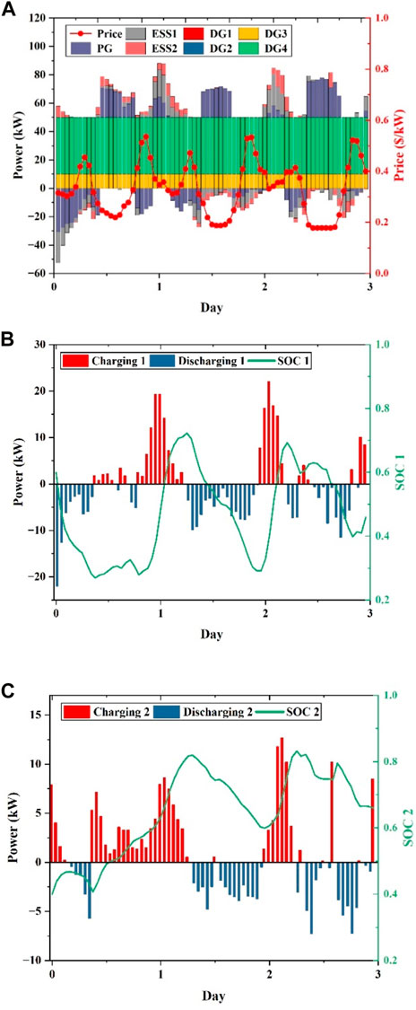
FIGURE 16. Scheduling results of the complex MG over three consecutive days in the test set: (A) Generation schedules of DGs, ESSs, and the main grid; (B) scheduled charging or discharging power and SOC of ESS 1; and (C) scheduled charging or discharging power and SOC of ESS 2.

4 Conclusion

MGs are an essential technology for integrating RESs and promoting the development of power systems. Optimal energy management strategies are necessary to achieve the economic operation of MG systems. To this end, a DRL-based approach is proposed to solve the optimal real-time energy management problem of MG systems. The real-time energy management problem of an MG is formulated as an MDP model considering the uncertainties of load, RES output, and electricity prices and solved by the DDPG approach, a policy-based DRL algorithm that does not rely on the knowledge of the uncertainty. Compared to conventional deterministic approaches, the proposed DRL method is data driven and does not rely on precise models of uncertainties. In contrast to the state-of-the-art DRL methods, the proposed DDPG method is capable of tackling complex decision-making problems with continuous action spaces, without requiring large storage memory for Q-value storage or probabilistic models for action sampling. A DNN is designed for the proposed DRL approach to learn the policy in an end-to-end manner and directly output the real-time continuous control signals. The performance and convergence of the proposed approach were evaluated by interacting with the simulated MG system. The results of simulation experiments demonstrated that the proposed approach could respond to the uncertainties in different system scenarios. In the second experiment of our simulation study, we compared the proposed DRL method with the DQN, SAC, PPO, and MPC methods. The results indicate that the DRL method is able to reduce the operating costs. The comparison of the scheduling results shows that the proposed approach can achieve much lower operating costs of the system than the baseline solutions, reducing them by 29.59%, 17.39%, 6.36%, and 9.55% on the June test set and 30.96%, 18.34%, 5.73%, and 10.16% on the November test set, respectively. The simulation results on a MG system containing more RES and ESS illustrate that the proposed approach can address the economic operation of more complex and dynamic MG systems. These findings demonstrate the superiority of the proposed DDPG method in optimizing the operating costs of MG systems and highlight its potential for practical application in realistic power system scenarios.

In this paper, we have analyzed the influence of the system parameters on the results, the hyperparameters of the DDPG algorithm can also affect the results, and there is no uniform conclusion. For future work, the impact of the algorithm’s hyperparameters on the operating cost of the system and the automatic rectification of hyperparameters should be considered to improve the performance of the algorithm.

Data availability statement

The original contributions presented in the study are included in the article/Supplementary Material. Further inquiries can be directed to the corresponding author.

Author contributions

DL, CZ, and PZ contributed to the conceptualization. DL, XW, and SX built the model. DL and WL were responsible for the software. DL visualized the results and wrote the original draft of the manuscript. DL and CZ reviewed and edited the manuscript. PZ supervised the research and managed the project. Access to funding was provided by PZ and YL. All authors have read and agreed to the published version of the manuscript.

Funding

This research was funded by the Liaoning Provincial Natural Science Foundation of China (2020-KF-11-02).

Conflict of interest

The authors declare that the research was conducted in the absence of any commercial or financial relationships that could be construed as a potential conflict of interest.

Publisher’s note

All claims expressed in this article are solely those of the authors and do not necessarily represent those of their affiliated organizations, or those of the publisher, the editors, and the reviewers. Any product that may be evaluated in this article, or claim that may be made by its manufacturer, is not guaranteed or endorsed by the publisher.

References

Abadi, M., Agarwal, A., Barham, P., Brevdo, E., Chen, Z., Citro, C., et al. (2015). TensorFlow: Large-scale machine learning on heterogeneous systems. Available at: https://www.tensorflow.org/(Accesssed August 22, 2022).

Google Scholar

Arwa, E. O., and Folly, K. A. (2020). Reinforcement learning techniques for optimal power control in grid-connected microgrids: A comprehensive review. Ieee Access 8, 208992–209007. doi:10.1109/access.2020.3038735

CrossRef Full Text | Google Scholar

Bian, H. F., Tian, X., Zhang, J., and Han, X. Y. (2020). “Deep reinforcement learning algorithm based on optimal energy dispatching for microgrid,” in Proceedings of the 2020 5th Asia Conference on Power and Electrical Engineering (ACPEE), 04-07 June 2020, Chengdu, China, 169–174.

CrossRef Full Text | Google Scholar

Cao, D., Hu, W. H., Zhao, J. B., Zhang, G. Z., Zhang, B., Liu, Z., et al. (2020). Reinforcement learning and its applications in modern power and energy systems: A review. J. Mod. Power Syst. Clean Energy 8 (6), 1029–1042. doi:10.35833/mpce.2020.000552

CrossRef Full Text | Google Scholar

Craparo, E., Karatas, M., and Singham, D. I. (2017). A robust optimization approach to hybrid microgrid operation using ensemble weather forecasts. Appl. Energy 201, 135–147. doi:10.1016/j.apenergy.2017.05.068

CrossRef Full Text | Google Scholar

Farhangi, H. (2010). The path of the smart grid. IEEE Power and Energy Mag. 8 (1), 18–28. doi:10.1109/mpe.2009.934876

CrossRef Full Text | Google Scholar

Faraji, J., Ketabi, A., Hashemi-Dezaki, H., Shafie-Khah, M., and Catalão, J. P. S. (2020). Optimal day-ahead self-scheduling and operation of prosumer microgrids using hybrid machine learning-based weather and load forecasting. IEEE ACCESS 8, 157284–157305. doi:10.1109/access.2020.3019562

CrossRef Full Text | Google Scholar

Fang, X., Misra, S., Xue, G. L., and Yang, D. J. (2012). Smart grid - the new and improved power grid: A survey. IEEE Commun. Surv. Tutorials 14 (4), 944–980. doi:10.1109/surv.2011.101911.00087

CrossRef Full Text | Google Scholar

Francois, V., Taralla, D., Ernst, D., and Fonteneau, R. (2016). "Deep reinforcement learning solutions for energy microgrids management."

Google Scholar

Guo, C. Y., Wang, X., Zheng, Y. H., and Zhang, F. (2022). Real-time optimal energy management of microgrid with uncertainties based on deep reinforcement learning. Energy 238, 121873. doi:10.1016/j.energy.2021.121873

CrossRef Full Text | Google Scholar

Gibilisco, P., Ieva, G., Marcone, F., Porro, G., and De Tuglie, E. (2018). “Day-ahead operation planning for microgrids embedding battery energy storage systems,” in Proceedings of the A case study on the PrInCE Lab microgrid. 2018 AEIT International Annual Conference, Bari, Italy, 03-05 October 2018.

Google Scholar

Hu, C. C., Cai, Z. X., Zhang, Y. X., Yan, R. D., Cai, Y., and Cen, B. W. (2022). A soft actor-critic deep reinforcement learning method for multi-timescale coordinated operation of microgrids. Prot. Control Mod. Power Syst. 7 (1), 29. doi:10.1186/s41601-022-00252-z

CrossRef Full Text | Google Scholar

Haarnoja, T., Zhou, A., Abbeel, P., and Levine, S. (2018). “Soft actor-critic: Off-policy maximum entropy deep reinforcement learning with a stochastic actor,” in Proceedings of the 35th International Confernece on Machine Learning, Stockholm, SWEDEN, 10-15 July 2018, 80.

Google Scholar

Ji, Y., Wang, J. H., Xu, J. C., Fang, X. K., and Zhang, H. G. (2019). Real-time energy management of a microgrid using deep reinforcement learning. Energies 12 (12), 2291. doi:10.3390/en12122291

CrossRef Full Text | Google Scholar

Jiang, C., Mao, Y., Chai, Y., and Yu, M. (2021). Day-ahead renewable scenario forecasts based on generative adversarial networks. Int. J. Energy Res. 45 (5), 7572–7587. doi:10.1002/er.6340

CrossRef Full Text | Google Scholar

Khosravi, M., Afsharnia, S., and Farhangi, S. (2022). Stochastic power management strategy for optimal day-ahead scheduling of wind-HESS considering wind power generation and market price uncertainties. Int. J. Electr. Power and Energy Syst. 134,107429 doi:10.1016/j.ijepes.2021.107429

CrossRef Full Text | Google Scholar

Khodayar, M., Liu, G. Y., Wang, J. H., and Khodayar, M. E. (2021). Deep learning in power systems research: A review. Csee J. Power Energy Syst. 7 (2), 209–220.

Google Scholar

Liang, J. K., and Tang, W. Y. (2020). Sequence generative adversarial networks for wind power scenario generation. Ieee J. Sel. Areas Commun. 38 (1), 110–118. doi:10.1109/jsac.2019.2952182

CrossRef Full Text | Google Scholar

Liu, J. Z., Chen, H., Zhang, W., Yurkovich, B., and Rizzoni, G. (2017). Energy management problems under uncertainties for grid-connected microgrids: A chance constrained programming approach. IEEE Trans. Smart Grid 8 (6), 2585–2596. doi:10.1109/tsg.2016.2531004

CrossRef Full Text | Google Scholar

Liu, C. H., Gu, J. C., and Yang, M. T. (2021). A simplified LSTM neural networks for one day-ahead solar power forecasting. Ieee Access 9, 17174–17195. doi:10.1109/access.2021.3053638

CrossRef Full Text | Google Scholar

Li, Z. M., and Xu, Y. (2018). Optimal coordinated energy dispatch of a multi-energy microgrid in grid-connected and islanded modes. Appl. Energy 210, 974–986. doi:10.1016/j.apenergy.2017.08.197

CrossRef Full Text | Google Scholar

Li, Z. W., Zang, C. Z., Zeng, P., and Yu, H. B. (2016). Combined two-stage stochastic programming and receding horizon control strategy for microgrid energy management considering uncertainty. Energies 9 (7), 499. doi:10.3390/en9070499

CrossRef Full Text | Google Scholar

Lillicrap, T. P., Hunt, J. J., Pritzel, A., Heess, N., Erez, T., Tassa, Y., et al. (2015). "Continuous control with deep reinforcement learning." arXiv e-prints: arXiv:1509.02971.

Google Scholar

Levent, T., Preux, P., Le Pennec, E., Badosa, J., Henri, G., Bonnassieux, Y., et al. (2019). “Energy management for microgrids: A reinforcement learning approach,” in Proceedings of the IEEE PES Innovative Smart Grid Technologies Europe (ISGT-Europe), Bucharest, Romania, 29 September 2019 - 02 October 2019, 1–5.

CrossRef Full Text | Google Scholar

Lin, S., Wang, H., Qi, L., Feng, H., and Su, Y. (2021). Short-term load forecasting based on conditional generative adversarial network. Automation Electr. Power Syst. 45 (11), 52–60.

Google Scholar

Lasseter, R. H. (2002). MicroGrids. 2002. New York, NY, USA: IEEE Power Engineering Society Winter Meeting.

Google Scholar

Muriithi, G., and Chowdhury, S. (2021). Optimal energy management of a grid-tied solar PV-battery microgrid: A reinforcement learning approach. Energies 14 (9), 2700. doi:10.3390/en14092700

CrossRef Full Text | Google Scholar

Mnih, V., Kavukcuoglu, K., Silver, D., Rusu, A. A., Veness, J., Bellemare, M. G., et al. (2015). Human-level control through deep reinforcement learning. Nature 518 (7540), 529–533. doi:10.1038/nature14236

PubMed Abstract | CrossRef Full Text | Google Scholar

Malik, P., Gehlot, A., Singh, R., Gupta, L. R., and Thakur, A. K. (2022). A review on ANN based model for solar radiation and wind speed prediction with real-time data. Archives Comput. Methods Eng. 29 (5), 3183–3201. doi:10.1007/s11831-021-09687-3

CrossRef Full Text | Google Scholar

OASIS California ISO Open access same-time information system. 2020.

Google Scholar

Ozcanli, A. K., Yaprakdal, F., and Baysal, M. (2020). Deep learning methods and applications for electrical power systems: A comprehensive review. Int. J. Energy Res. 44 (9), 7136–7157. doi:10.1002/er.5331

CrossRef Full Text | Google Scholar

Papathanassiou, S., Hatziargyriou, N., and Strunz, K. (2005). "A benchmark low voltage microgrid network." CIGRE Symposium.

Google Scholar

Prodan, I., and Zio, E. (2014). A model predictive control framework for reliable microgrid energy management. Int. J. Electr. Power and Energy Syst. 61, 399–409. doi:10.1016/j.ijepes.2014.03.017

CrossRef Full Text | Google Scholar

Silver, D., Huang, A., Maddison, C. J., Guez, A., Sifre, L., van den Driessche, G., et al. (2016). Mastering the game of Go with deep neural networks and tree search. Nature 529 (7587), 484–489. doi:10.1038/nature16961

PubMed Abstract | CrossRef Full Text | Google Scholar

Silva, J. A. A., Lopez, J. C., Arias, N. B., Rider, M. J., and da Silva, L. C. P. (2021). An optimal stochastic energy management system for resilient microgrids. Appl. Energy 300, 117435. doi:10.1016/j.apenergy.2021.117435

CrossRef Full Text | Google Scholar

Silver, D., Lever, G., Heess, N., Degris, T., Wierstra, D., and Riedmiller, M. (2014). “Deterministic policy gradient algorithms,” in Proceedings of the 31st International Conference on Machine Learning, Beijing, China, June 2014.

Google Scholar

Sutton, R. S., and Barto, A. G. (1998). Reinforcement learning: An introduction. London, England, The MIT Press,

Google Scholar

Sutton, R. S., and Barto, A. G. (2018). Reinforcement learning: An introduction. London, England: The MIT Press.

Google Scholar

Sutton, R. S., McAllester, D., Singh, S., and Mansour, Y. (2000)., 12. Leuven, Belgium, 1057–1063.Policy gradient methods for reinforcement learning with function approximationAdv. Neural Inf. Process. Syst.

Google Scholar

Shi, Y., Tuan, H. D., Savkin, A. V., Duong, T. Q., and Poor, H. V. (2019). Model predictive control for smart grids with multiple electric-vehicle charging stations. IEEE Trans. Smart Grid 10 (2), 2127–2136. doi:10.1109/tsg.2017.2789333

CrossRef Full Text | Google Scholar

Shang, Y. W., Wu, W. C., Guo, J. B., Ma, Z., Sheng, W. X., Lv, Z., et al. (2020). Stochastic dispatch of energy storage in microgrids: An augmented reinforcement learning approach. Appl. Energy 261, 114423. doi:10.1016/j.apenergy.2019.114423

CrossRef Full Text | Google Scholar

Thirugnanam, K., Kerk, S. K., Yuen, C., Liu, N., and Zhang, M. (2018). Energy management for renewable microgrid in reducing diesel generators usage with multiple types of battery. IEEE Trans. Industrial Electron. 65 (8), 6772–6786. doi:10.1109/tie.2018.2795585

CrossRef Full Text | Google Scholar

Vergara, P. P., Lopez, J. C., Rider, M. J., Shaker, H. R., da Silva, L. C. P., and Jorgensen, B. N. (2020). A stochastic programming model for the optimal operation of unbalanced three-phase islanded microgrids. Int. J. Electr. Power and Energy Syst. 115, 105446. doi:10.1016/j.ijepes.2019.105446

CrossRef Full Text | Google Scholar

Watkins, C., and Dayan, P. (1992). Q-LEARNING. Mach. Learn. 8 (3-4), 279–292. doi:10.1023/a:1022676722315

CrossRef Full Text | Google Scholar

Xia, Y., Xu, Y., Wang, Y., Mondal, S., Dasgupta, S., Gupta, A. K., et al. (2022). A safe policy learning-based method for decentralized and economic frequency control in isolated networked-microgrid systems. IEEE Trans. Sustain. Energy 13 (4), 1982–1993. doi:10.1109/tste.2022.3178415

CrossRef Full Text | Google Scholar

Yan, R., Wang, Y., Xu, Y., and Dai, J. (2022). A multiagent quantum deep reinforcement learning method for distributed frequency control of islanded microgrids. IEEE Trans. Control Netw. Syst. 9 (4), 1622–1632. doi:10.1109/tcns.2022.3140702

CrossRef Full Text | Google Scholar

Yang, T., Zhao, L. Y., Li, W., and Zomaya, A. Y. (2020). Reinforcement learning in sustainable energy and electric systems: A survey. Annu. Rev. Control 49, 145–163. doi:10.1016/j.arcontrol.2020.03.001

CrossRef Full Text | Google Scholar

Yu, Y. J., Qin, Y., and Gong, H. C. (2021). A fuzzy Q-learning algorithm for storage optimization in islanding microgrid. J. Electr. Eng. Technol. 16 (5), 2343–2353. doi:10.1007/s42835-021-00769-7

CrossRef Full Text | Google Scholar

Yoldas, Y., Goren, S., and Onen, A. (2020). Optimal control of microgrids with multi-stage mixed-integer nonlinear programming guided Q-learning algorithm. J. Mod. Power Syst. Clean Energy 8 (6), 1151–1159. doi:10.35833/mpce.2020.000506

CrossRef Full Text | Google Scholar

Zeng, P., Li, H. P., He, H. B., and Li, S. H. (2019). Dynamic energy management of a microgrid using approximate dynamic programming and deep recurrent neural network learning. IEEE Trans. Smart Grid 10 (4), 4435–4445. doi:10.1109/tsg.2018.2859821

CrossRef Full Text | Google Scholar

Zhang, Y., Zhang, T., Wang, R., Liu, Y. J., and Guo, B. (2015). Optimal operation of a smart residential microgrid based on model predictive control by considering uncertainties and storage impacts. Sol. Energy 122, 1052–1065. doi:10.1016/j.solener.2015.10.027

CrossRef Full Text | Google Scholar