 Bosong Zou1Huijie Wang1Tianyi Zhang2Mengyu Xiong2Chang Xiong2Qi Sun3
 Wentao Wang2*Lisheng Zhang2*Cheng Zhang4
 Haijun Ruan4*
- 1China Software Testing Center, Beijing, China
- 2School of Transportation Science and Engineering, Beihang University, Beijing, China
- 3China First Automobile Group Corporation, Beijing, China
- 4Institute for Clean Growth and Future Mobility, Coventry University, Coventry, United Kingdom
Accurate estimation of the State of Health (SOH) of lithium-ion batteries is crucial for ensuring their safe and reliable operation. Data-driven methods have shown excellent performance in estimating SOH, but obtaining high-quality and strongly correlated features remains a major challenge for these methods. Moreover, different features have varying importance in both spatial and temporal scales, and single data-driven models are unable to capture this information, leading to issues with attention dispersion. In this paper, we propose a data-driven method for SOH estimation leveraging the Bi-directional Long Short-Term Memory (Bi-LSTM) that uses the Differential Thermal Voltammetry (DTV) analysis to extract features, and incorporates attention mechanisms (AM) at both temporal and spatial scales to enable the model focusing on important information in the features. The proposed method is validated using the Oxford Battery degradation Dataset, and the results show that it achieves high accuracy and robustness in SOH estimation. The Root Mean Squared Error (RMSE) and Mean Absolute Error (MAE) are around 0.4% and 0.3%, respectively, indicating the potential for online application of the proposed method in the cyber hierarchy and interactional network (CHAIN) framework.
1 Introduction
The growing demand for energy and environmental pollution pose urgent requirements for the development of new energy sources. LIBs, due to their high energy density, wide operating range, strong temperature adaptability and long cycle life, are widely used in automobiles, electronic devices and spacecraft (Pang et al., 2021; Liu et al., 2022). During the usage of LIBs, degradation occurs due to internal side reactions, and failed LIBs need to be replaced in a timely manner to ensure safe usage (Gao et al., 2021; Zhang et al., 2022a). Therefore, accurate estimation of the health status of batteries is crucial for ensuring the safety of LIBs, as well as for improving efficiency and reducing costs (Zhou et al., 2021; Deng et al., 2023). However, as batteries are highly complex, time-varying and nonlinear electrochemical systems, it remains a significant challenge to establish a reliable Battery Management System (BMS) to accurately estimate the health status of LIBs (Zhang et al., 2022b; You et al., 2022; Ruan et al., 2023).
Currently, the estimation of the SOH of LIBs can be roughly divided into direct measurement methods, model-based methods, and data-driven methods (Ma et al., 2022; Jin et al., 2023).
The direct measurement method usually estimates the SOH of the battery by measuring the electrochemical impedance spectrum of the battery, open circuit voltage (OCV), or by using the ampere-hour integral method. As the internal resistance of the battery increases with degradation, the SOH of the battery can be estimated by measuring its electrochemical impedance spectrum. OCV can be directly measured and used to estimate SOH through its fitting relationship with the capacity. The ampere-hour integral method estimates SOH by measuring the current and integrating it over time. The direct measurement method has high accuracy, but it requires high measurement conditions and instruments, making it suitable for laboratory environments and difficult to apply in real-world vehicle applications.
Model-based methods, including equivalent circuit model (ECM), electrochemical mechanism model, and empirical model, are used to estimate the SOH of LIBs. The ECM method simulates the operation process of the battery using circuit components such as resistors, power sources and capacitors, and estimates SOH through model parameter identification methods such as Kalman filtering algorithm. The electrochemical model method builds an electrochemical model from the internal degradation mechanism of the battery to estimate SOH. The empirical model method estimates SOH by constructing an empirical relationship between the SOH and other measurable macroscopic physical quantities. Yan et al. (2017) estimated the SOH of a battery by establishing a second-order ECM and estimating the Ohmic resistance through adaptive unscented kalman filter (AUKF), and then mapping the resistance and SOH relationship. Lyu et al. (2017) proposed a framework combining the electrochemical model and particle filter (PF) algorithm to estimate battery degradation. Singh et al. (2019) developed a semi-empirical model that achieved fast and accurate SOH estimation by using charge-discharge cycle number and current as inputs; Zeng et al. (2019) established an improved second-order ECM model and used Bayesian for online parameter identification, using the fuzzy unscented Kalman filtering algorithm for SOH estimation. Yan et al. (2019) improved the extended Kalman filter based on Lebesgue sampling and efficiently estimated SOH using second-order ECM. Li et al. (2018) proposed an single particle (SP) model that considers the physical mechanism of battery aging for capacity estimation. ECM and electrochemical model-based methods usually have high accuracy and strong interference resistance as closed-loop systems, but building an accurate battery model might be complex, and the established battery model may only perform well under specific conditions. Model parameters also need to be adjusted in a timely manner with changes in the working environment and conditions to ensure accuracy. Empirical model-based methods have high real-time applicability due to their simplicity and fast computation speed. However, the accuracy of empirical models is often limited and cannot fully reflect the degradation process (Chen et al., 2022).
In recent years, with the development of various devices and hardware, the computing power and data acquisition technology of computers have made significant leaps, and various databases have emerged. Data-driven methods have gradually become very popular in various industries (Wu et al., 2015; Wang et al., 2022). These methods do not require knowledge of complex electrochemical mechanisms or the construction of complex mathematical models, but are based on data to extract features highly correlated with battery degradation contained in macroscopic signals completely, and establish nonlinear relationships between these features and battery degradation. This makes it easier to achieve high-accuracy estimations. For example, Wang et al. (2022) implemented high-accuracy SOH estimation based on the modified Gaussian process regression (GPR) method. Lin et al. (2022a) used the random forest algorithm to fuse three machine learning algorithms (Support vector machine (SVM), multiple linear regression (MLR) and GPR) to further improve the estimation accuracy. In addition to traditional machine learning algorithms, deep learning algorithms, which have developed rapidly in recent years, are gradually becoming popular and widely used. Eddahech et al. (2012) used recurrent neural network (RNN) to estimate the SOH of lithium batteries. RNN is good at solving time series problems and is suitable for estimating battery SOH. For long-term dependency problems, the effect of RNN is greatly reduced, while its variant LSTM can make up for this deficiency. Zhang et al. (2018) used LSTM to achieve high-accuracy estimation of the SOH and RUL of lithium-ion batteries. Deng et al. (2022) identified degradation patterns based on the early degradation data of batteries and applied transfer learning to further improve the accuracy of SOH estimation, and realized high-accuracy SOH estimation based on LSTM network. Deng et al. (2023) determined the label capacity based on statistical values of capacity and extracted features from charging data, using a sequence to sequence model combined with a GPR based residual model to estimate SOH. Deep learning methods do not require knowledge of the complex internal mechanisms of batteries and can model non-linear dynamics well. However, the estimation accuracy of data-driven methods is highly dependent on the amount and quality of data. To address the problem of insufficient available data, Shen et al. (2020) implemented high-accuracy battery SOH estimation by using DCNN combined with transfer learning and ensemble learning methods, which can be further expanded based on small data sets. Traditional data-driven methods are often difficult to use with data that do not have SOH labels. Xiong et al. (2023) proposed a data-driven method based on semi-supervised learning to fully utilize these unlabeled data, which are usually easy to obtain and have a large amount of data. Apart from the limited availability of data from lithium-ion batteries, extracting high-quality features strongly correlated with battery degradation from large amounts of data is also a challenging task. Many signal analysis techniques are commonly used as auxiliary tools to extract features. Signal analysis methods combine the measurable macroscopic signals of batteries with the internal chemical reaction process of battery degradation to obtain features strongly related to battery degradation. Commonly used methods include independent component analysis (ICA) and DTV methods. ICA method analyzes the relationship between voltage and capacity changes in charge-discharge cycles, and reflects battery degradation through the evolution of peaks and valleys in the curve. Li et al. (2020) proposed a multi-timescale framework based on ICA method to estimate the SOH of batteries by extracting highly correlated features related to battery degradation from the ICA curve, and using the GPR algorithm to estimate the SOH of batteries. Sun et al. (2022) used the empirical mode decomposition (EMD)-ICA-gate recurrent unit (GRU) method to decompose capacity data through the EMD method, extract features through the ICA method, and estimate the SOH of batteries using the GRU algorithm. Microscopic phase changes that occur inside batteries during degradation lead to entropy changes. The DTV analysis method extracts information related to entropy changes in the charging and discharging process by analyzing the relationship between temperature and voltage and can reflect the internal changes in the battery degradation process through measurable macroscopic signals (Wu et al., 2015; Merla et al., 2016a; Merla et al., 2016b). The DTV curve gradually changes with battery degradation, and features with a high correlation with the SOH of the battery can be extracted from the DTV curve. The implementation of the DTV method does not require complex and expensive measurement instruments, only the battery voltage and surface temperature are needed, thus it has potential for practical applications.
The technology route of extracting highly correlated features with battery degradation through signal analysis techniques and training and estimation through data-driven methods can achieve high-accuracy SOH estimation (Ma et al., 2022; Zhang et al., 2023). Lin et al. (2023) extracted multiple features based on ICA and voltage curves, and used an improved GPR model for SOH estimation. Xu et al. (2023) extracted features based on ICA and voltage and temperature curves, and estimated SOH using an ensemble learning framework. Lin et al. (2022b) used differential temperature capacity method for feature extraction and combined simulated annealing algorithm with support vector regression to estimate SOH. However, facing numerous features that can be extracted through signal analysis techniques, selecting the most relevant features is another challenge. Although correlation analysis methods can be used to select highly correlated features, the correlation analysis can only reflect the correlation between features and battery degradation throughout the entire lifecycle of the battery. The importance of the information contained in different features at different spatial and temporal scales for local changes varies widely, making it difficult to conduct refined research on them in practical applications. This can result in the problem of scattered attention of deep learning models, making it difficult to fully extract more information related to battery degradation from the data.
In order to address the aforementioned issues and achieve high-accuracy SOH estimation and improve the more comprehensive exploration and utilization of limited data, this paper proposes an SOH estimation method that combines DTV method and deep learning algorithm with the addition of an AM. Firstly, based on the degradation dataset of LIBs in the Oxford University database, data preprocessing and DTV analysis are performed. Peaks and valleys are extracted from the DTV curves as features and high-correlation features related to battery degradation are selected using the Pearson correlation analysis method. Then, a deep learning model is built based on Bi-LSTM and trained based on the selected features. Two layers of AM are added to the model to further explore the information contained in the data from both spatial and temporal scales, and focus on the important features. Finally, the trained model is applied to SOH estimation, and the proposed method is validated based on error analysis. The results show that the DTV analysis method can effectively extract features highly correlated with battery degradation from the data and can be combined with deep learning models to optimize the SOH estimation process, achieving high accuracy. Different features have varying degrees of correlation with battery degradation on the spatial and temporal scales, and the AM can effectively explore the information contained in the data during the local degradation process, focus on the most important information and effectively solve the problem of attention dispersion. In the CHAIN framework, the proposed model can achieve high-accuracy offline SOH estimation and has the potential for real-time online application, contributing to the development of the next-generation cloud BMS (Yang et al., 2020; Yang et al., 2021).
The remaining sections of this paper are arranged as follows: Section 2 describes the battery degradation dataset, data processing and feature extraction process. Section 3 describes the principles of the model and algorithms used in this paper and provides a detailed description of the entire model framework. Section 4 validates the proposed method and analyzes the error. Section 5 summarizes the main conclusion of this paper.
2 Degradation data and preprocessing
2.1 Dataset description
The lithium-ion battery degradation data set from the Oxford University database is utilized in this paper (Birkl, 2017a; Birkl, 2017b). The whole data set contains data from 8 batteries. Which are labelled from #1 to #8. The technical specifications and experimental conditions of the batteries are listed in Table 1 in detail. Figures 1A, B describe the voltage, current and temperature data and battery capacity degradation curves. The battery #1, #3, #4, #7 and #8 are used for this paper, because other batteries did not fall below EOL, and could not be fully evaluated or the capacity curve drop sharply.
TABLE 1. Specific degradation experiment conditions of the batteries.
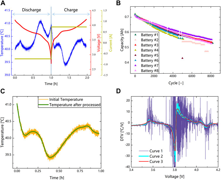
FIGURE 1. Battery degradation cycle schemes and data preprocessing. (A) Degradation test of voltage, current and temperature. (B) Capacity degradation profiles of the eight batteries. (C) Temperature processed by SG filter (battery #1). (D) DTV processed by data preprocessing, curve1 is the origin DTV curve, curve2 is the DTV curve processed by fixing sampling interval and curve3 is the DTV curve processed by SG filter (battery #1).
The definition of SOH can be divided into the definition of capacity and the definition of internal resistance. The definition of SOH can usually be described as:
Where
In this paper, the definition of SOH is selected from the perspective of capacity. Based on the data in the data set, the reference capacity is determined by Ampere-hour integration method.
2.2 Data preprocessing
Battery degradation is accompanied by microstructural changes, which in turn lead to entropy changes. DTV analysis can reflect information related to entropy changes during the degradation process of lithium-ion batteries. This method can establish a connection between macroscopic signals and microstructural changes by analyzing changes in temperature and voltage, and can be used to reflect battery degradation. The DTV methods could be calculated as follows:
Where T represents the battery surface temperature, and V the battery terminal voltage.
During data collection, noise and outliers can be introduced due to fluctuations in the signal and sensor errors. As shown in Figure 1A, there is a large amount of noise in the temperature data. To address this issue, data preprocessing is performed. Firstly, the sampling interval is adjusted to avoid amplifying the impact of noise. A sampling interval of 20 s is chosen based on a balance between noise reduction and information loss. Secondly, an SG filter is applied to the temperature data for smoothing. The SG filter is well-suited for our application as it has an excellent ability to capture peaks and valleys in waveform. In our study, the peaks and valleys extracted from the DTV curve are used as features for subsequent analysis (Chen et al., 2004). The SG filter could be described as follows:
Where y represents the smoothed signal, Cj the coefficient of the SG filter, Nc is equal to the smoothing window size (2p+1) and x the original signals.
Based on the data processing steps described, the results are shown in Figures 1C, D. After the data preprocessing, the temperature data is significantly smoother, and the DTV curve has reduced noise. However, some noise still exists in the DTV curve, and the SG filter is used to further smooth the curve, as shown in Figure 1D, resulting in a smoother DTV curve.
2.3 Features extraction and correlation analysis
In this section, the feature extraction on the DTV curve obtained after data preprocessing is conducted. Figure 2A shows the changes in the DTV curve with battery degradation. It can be observed that with battery degradation, the peaks and valleys in the DTV curve experience significant shifts. The peak values of the two peaks decrease, and their positions shift higher, while the valley values decrease and their positions shift higher as well. These changes in peaks and valleys are strongly related to battery degradation, further demonstrating that the DTV method can reflect the micro changes in battery degradation through macroscopic signals and thus can be used as a tool to assist SOH estimation. Therefore, we extracted the peak and valley information from the DTV curve as features to input into the deep learning model for SOH estimation. A total of six features, including the peak values and positions of the two peaks and the valley values and positions of one valley, are extracted from the DTV curve. Figure 2B shows the schematic diagram of the feature extraction process. The mathematical expression of the feature can be described as follows:
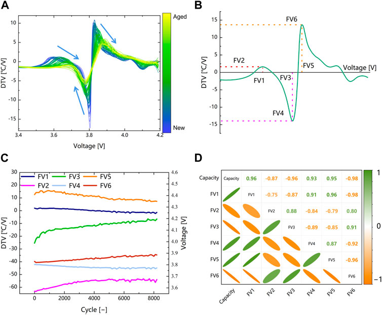
FIGURE 2. Features extraction and correlation analysis. (A) Degradation evolution of DTV curves. (B) Schematic diagram of feature extraction. (C) Evolution of characteristics with battery degradation. (D) The result of Pearson correlation analysis (battery #1).
Where f(∙) is the mapping relationship of DTV and voltage.
The changes in the extracted features are shown in Figure 2C, and further Pearson correlation analysis is performed on the extracted features to select highly correlated features to improve the estimation accuracy and training efficiency. The Pearson correlation analysis can be described as follows:
where x and y are the variable and n the number of sample points.
The results are shown in Figure 2D and Table 2, where it can be observed that FV1, FV3, and FV6 exhibit high correlation on all batteries, with correlation coefficients above 90%. Particularly, for FV6, the correlation coefficient is above 95%. Therefore, we select FV1, FV3, and FV6 as features to be input into the model for SOH estimation, in order to improve estimation accuracy and training efficiency.
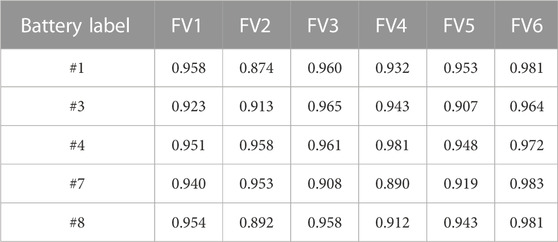
TABLE 2. Pearson correlation coefficient.
3 Methodology
3.1 Bi-LSTM network
Battery degradation is a typical time series problem. RNN is a good choice for dealing with time series problems. However, in long-term time series problems, RNN has the problems of gradient disappearance and gradient explosion. LSTM is a variant of RNN, and the main structure of LSTM is similar to RNN(Greff et al., 2017). The forgetting gate, input gate and output gate are added in the hidden layer, which can be better applied to long-term time series problems. The structure of LSTM unit is shown in Figure 3A. The calculation of each LSTM unit can be described as follows:
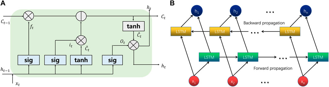
FIGURE 3. The structural diagram of LSTM and Bi-LSTM. (A) The structural diagram of LSTM. (B) The structural diagram of Bi-LSTM.
Firstly, the LSTM units receive the
Where
Then, the input sequence data at current position is processed by the input gate and the input gate will determine which information to be updated and added to the cell state through the sigmoid function. The tanh function is used to generate new candidate vectors, and the information which to be reserved will be added to the cell state. The input gate is calculated as follows:
Next, the unit state update from
Where
Finally, the sigmoid function determines which part of the information to be output, and the cell state is processed by the tanh function. The result of multiplying the two parts is the final output:
Where
The structure of Bi-LSTM is shown in Figure 3B, which consists of two independent LSTM networks. The input time series are fed into two LSTM neural networks in forward and backward order respectively. The output vectors from the two networks are concatenated to form the final feature representation for the current sequence position. The core idea of Bi-LSTM is to add information from both the future and the past to the features of current sequence position, thus combining the bidirectional correlations of the data to more effectively explore the time series features hidden in the data and achieve higher efficiency and superior performance compared to a single LSTM. In this paper, a deep learning model based on Bi-LSTM is constructed to achieve high-accuracy SOH estimation.
3.2 Attention mechanism
Using features highly correlated with SOH is crucial for achieving high-accuracy SOH estimation in deep learning models. Although correlation analysis methods can screen out features strongly correlated with SOH, they can only select these features throughout the entire life cycle of the battery, while these features have different impacts on the estimation results at local positions in spatial and temporal scales. However, deep learning models tend to disperse attention among various features, resulting in a lack of capturing important features. To address this issue, this paper introduces AM into the deep learning model to improve its performance. The AM assigns weights to the features to enable the model to focus more on important information by calculating the correlation between each element in the input sequence and assigning weights to each element (Vaswani et al., 2017). The input features pass through a fully connected layer to obtain a feature vector, which is then compared for similarity with itself to obtain the weight of each element. The weights of important features will be higher, while the weights of unimportant features will be lower. Finally, these weights are multiplied by the input features to obtain the newly weighted features. The structure of the AM is shown in Figure 4A, and the overall framework of the deep learning model with AM is shown in Figure 4B. The AM can be described as follows:
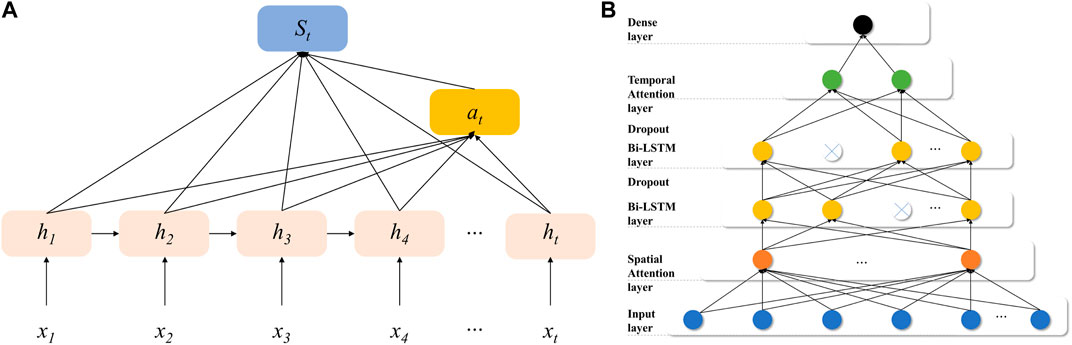
FIGURE 4. The structural diagram of (A) Attention mechanism and (B) The whole deep learning model.
Where
The input features are firstly weighted by the spatial AM. The structure of the spatial AM is essentially a multi layer perceptron (MLP) network, and the parameters in the network are also trained during the model training process. The
3.3 Input and output structure
Figure 5 illustrates the structure of the input and output data. The data is constructed as a time series and input into the network. Firstly, the three features are taken and formed into a two-dimensional matrix based on a fixed window length, which is called the time series length represented as N in the figure. This two-dimensional matrix represents the time series, and the window is moved downward based on a fixed step length. The data is eventually divided into multiple time series. For the kth time series, the estimated target value is the SOH of the (k + N)-th cycle. Then, several time series are selected to form a three-dimensional tensor, and the number of selected time series is called the batch size. The constructed three-dimensional tensor is called a batch, which is input into the network for training based on the batch unit.

FIGURE 5. Timeseries construction.
3.4 Framework of the proposed SOH estimation model
The overall framework of the proposed method is illustrated in Figure 6. The entire process is divided into four parts. Firstly, data preprocessing is performed, which is described in detail in Subsection 2.2. The preprocessed data is then used to calculate the DTV curve, which is further processed to extract the peaks and valleys of the DTV curve as features. The feature data is then constructed in a time-series format. Subsequently, the constructed time-series data is fed into a deep learning model for training. The deep learning model is based on Bi-LSTM and includes dropout techniques to prevent overfitting. Two layers of AM are also incorporated to focus on the important information in the data for optimizing estimation accuracy. The RMSprop technique is utilized for optimization during the training process. Finally, the trained model is used for estimating the SOH and for error analysis. The estimated results are compared with the ground truth values and are quantitatively analyzed and compared using RMSE and MAE as evaluation metrics. The RMSE and MAE can be calculated as follows:
where
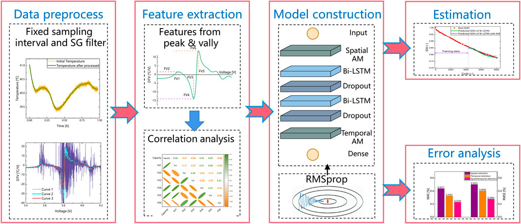
FIGURE 6. The framework of the proposed method.
4 Result and discussion
In this section, the proposed method is validated and error analysis is performed. First, the influence of the proportion of the training and testing set on estimation accuracy is studied to select the optimal data set split portions that balances accuracy and early estimation ability. Then, the optimization effect of applying the AM on the temporal and spatial scales for estimation accuracy is compared. Finally, the robustness of the proposed method is verified.
4.1 Estimation results of Bi-LSTM under different data split proportion
In this subsection, the influence of the dataset split portions on the SOH estimation accuracy is studied to determine the optimal ratio that balances the accuracy and early estimation ability. The estimation results are shown in Figure 7. When the dataset is split into portions of 4:6, 5:5 and 6:4, the RMSE of the estimation results are below 0.8%, and the MAE are below 0.7%, demonstrating that the DTV method can establish a strong correlation with battery degradation and achieve high-accuracy SOH estimation when combined with deep learning methods. It can also be seen that with an increase in the amount of training data, the accuracy of SOH estimation gradually improves, as more training data allows the model to fully learn the distribution pattern of the data. Although more training data can improve the accuracy, it can greatly compromise the early estimation ability of the model. Therefore, the choice of dataset split portions should balance both accuracy and early estimation ability. The split portions of 5:5 showed an significant improvement in the performance compared to 4:6, with an error improvement of 30.3%. However, the split portions of 6:4 showed only a small error improvement of 6.9% compared to 5:5, with a compromise in early estimation ability. Therefore, the dataset split portions of 5:5 is chosen for the following experiments in this paper.
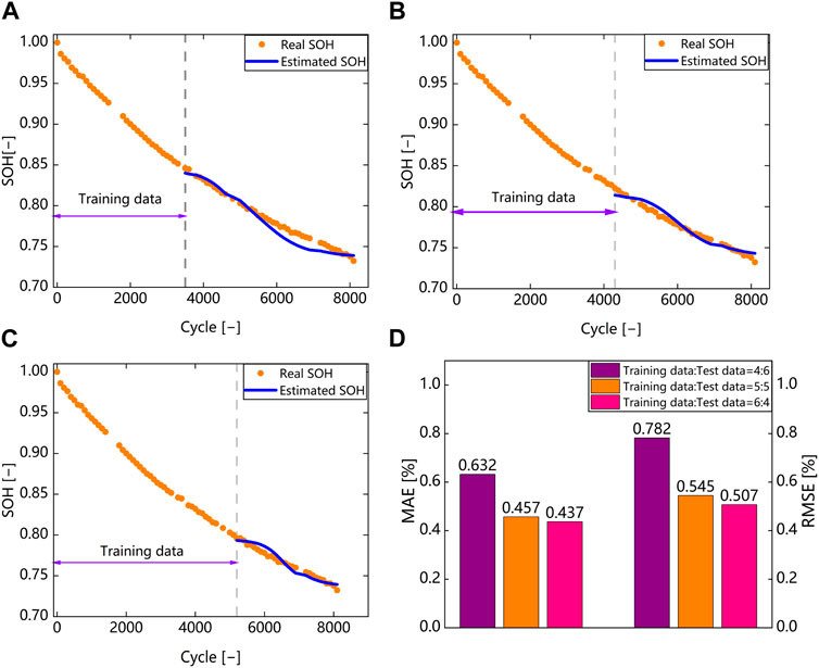
FIGURE 7. SOH estimation results under different data split proportion. (A) Estimation result with split proportion of 4: 6 (battery #1). (B) Estimation result with split proportion of 5: 5 (battery #1). (C) Estimation result with split proportion of 6: 4 (battery #1). (D) MAE and RMSE analysis.
4.2 Estimation result with attention mechanism
In this section, the information contained in the features is further explored by incorporating the AM into the Bi-LSTM model. Firstly, the effect of adding AM at different scales, including temporal, spatial, and spatiotemporal scales, are compared on a the battery #1 to capture the importance of information at different scales. Then, the proposed method is validated on other batteries. In this evaluation, the battery #1, #3, #4, #7 and #8 are used, because other batteries did not fall below EOL, and could not be fully evaluated, or the capacity curve drop sharply.
Figure 8 shows the estimation results using Battery 1 with the AM added at different scales. The curve descriptions are the same as described in the previous subsection. It can be seen that the RMSE and MAE of the estimation results with AM added at spatial scale are 0.503% and 0.442%, respectively. The RMSE and MAE of the estimation results with AM added at temporal scale are 0.405% and 0.328%, respectively. The estimation accuracy is higher than that without AM. This indicates that AM can further explore more information from the features and focus more on important features locally, thus improving estimation accuracy. Moreover, it is noted that the improvement in estimation accuracy by adding AM at temporal scale is greater than that at spatial scale. This indicates that the features selected by the correlation analysis method have small differences at spatial scale and have a good correlation with battery degradation. The RMSE and MAE of the estimation results with the addition of the AM on the spatiotemporal scale are 0.281% and 0.233% respectively, and the estimation accuracy is higher than that of the estimation results with the application of the AM on the spatial or temporal scale alone. Compared with the model without the addition of the AM, the RMSE and MAE of the estimation results are reduced by 0.265% and 0.224% respectively, and the error improvement of the RMSE and MAE are 48.6% and 49% respectively, which indicates that the addition of the AM at spatiotemporal scale can fully combine the advantages of both spatial and temporal scales to achieve better optimization effects.
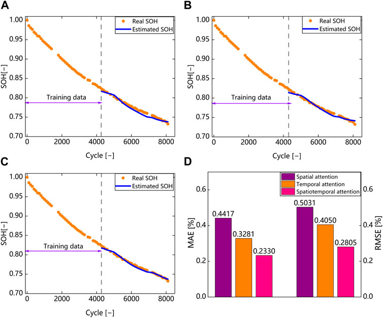
FIGURE 8. SOH estimation results with attention mechanism. (A) Estimation result with spatial attention (battery #1). (B) Estimation result with temporal attention (battery #1). (C) Estimation result with spatiotemporal attention (battery #1). (D) MAE and RMSE analysis.
Then, the proposed method is verified on different batteries, and the estimation results are shown in Figure 9. The results show that the proposed method achieved satisfactory estimation accuracy for all batteries, with RMSE below 0.6% and MAE below 0.5%. In particular, for battery #8, the RMSE and MAE are only 0.318% and 0.251% respectively, and the error improvements are all about 10%. In conclusion, the AM can reasonably allocate weights to features with different importance at spatial and temporal scales, allowing the model to capture more important underlying information and achieve high-accuracy SOH estimation.
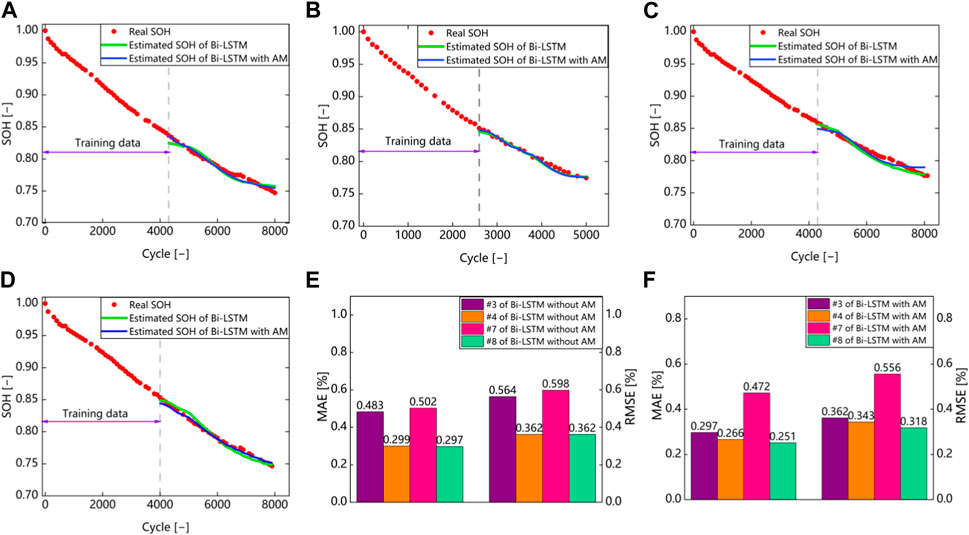
FIGURE 9. SOH estimation results of different batteries. (A) Estimation result of battery #3. (B) Estimation result of battery #4. (C) Estimation result of battery #7. (D) Estimation result of battery #8. (E) MAE and RMSE analysis of the model without AM. (F) MAE and RMSE analysis of the model with AM.
4.3 Validation of robustness
In this subsection, the robustness of the proposed method is validated, and the estimation results are shown in Figure 10. The blue dot line represents the real value of SOH, and the red line represents the estimated value of SOH. In the robustness validation, different starting cycles of the batteries are applied by discarding the first 20% of the data, and the validation was conducted on all batteries. The RMSE and MAE analysis are presented in Figure 10F. The results show that the RMSE and MAE of the estimation results are distributed around 0.25% and 0.2%, respectively, under different starting cycles of the batteries. The RMSE and MAE of the estimation results only differ by 0.1% compared to the normal condition, indicating that the proposed method exhibits stable performance and strong robustness under different starting cycles of the batteries.
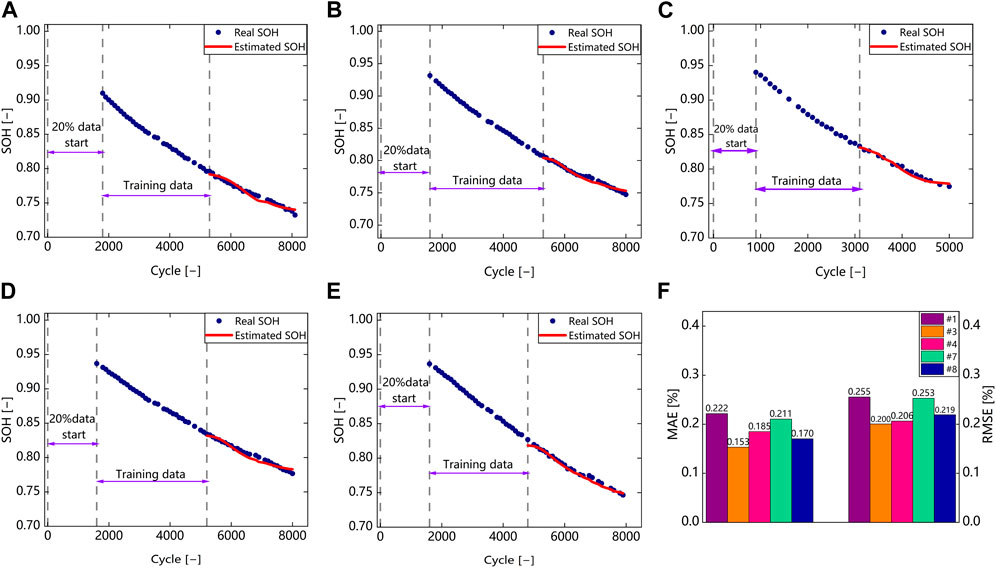
FIGURE 10. Validation of the robustness. (A) Estimation result of battery #1. (B) Estimation result of battery #3. (C) Estimation result of battery #4. (D) Estimation result of battery #7. (E) Estimation result of battery #8. (F) MAE and RMSE analysis.
In this subsection, a cross validation method is also used to validate the proposed model. The specific approach is to use data from one battery as the test set, while data from other batteries as the training set. When dividing data on the same battery data, due to the similar data distribution, the high-precision estimation results may be caused by overfitting. By leaving a cross validation, the performance of the model can be more accurately verified and the limited amount of data can be fully utilized. Figure 11 shows the results of leaving a cross validation. The results show that the method proposed in this article still achieves high accuracy despite leaving a cross validation, with estimated RMSE below 0.5% and MAE below 0.4%. It is also noted that the accuracy of the estimation results on each battery has a small difference, indicating that the inconsistency between batteries has a small impact on the estimation results. It indicates that the method proposed in this article has strong generalization in situations with abundant data volume.
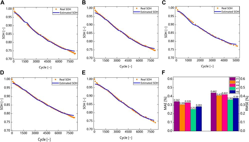
FIGURE 11. Leave-one-out cross-validation results. (A) Estimation result of battery #1. (B) Estimation result of battery #3. (C) Estimation result of battery #4. (D) Estimation result of battery #7. (E) Estimation result of battery #8. (F) MAE and RMSE analysis.
5 Conclusion
This paper proposes a data-driven method for estimating the SOH of LIBs. In practice, battery data is preprocessed through data cleaning, fixed sampling intervals and filtering. The DTV method is used to extract features from the data, and then feature selection is performed through Pearson correlation analysis. The deep learning model includes two Bi-LSTM layers and dropout technology to prevent overfitting. The temporal AM and spatial AM are added to the deep learning model to assign weights at different scales. Finally, the trained model is used for estimation, and RMSE and MAE are used as error indicators for error analysis. The results show that the proposed method can achieve high-accuracy SOH estimation, with an RMSE of about 0.4% and an MAE of about 0.3%. Adding AM can bring error improvement about 10%, and the proposed method has strong robustness under different battery start-up cycles, with an RMSE and MAE difference of only 0.1% compared to the estimation results from 0 starting points.
The main contributions of this paper are as follows:
(1) The DTV analysis method can establish the connection between micro-phase transitions during battery degradation and macro signals, and obtain high-quality features strongly correlated with battery degradation through DTV analysis. (2) The AM is added to the deep learning model at both the temporal and spatial scales to assign weights, making the model more focused on the important parts of the features. (3) This model has high accuracy and strong robustness, with estimation errors within 0.3% in different start-up cycles. The proposed method has the potential for online applications under the CHAIN framework and can be combined with cloud BMS and end-cloud collaboration framework for further realization of high-accuracy and real-time battery SOH estimation in practical applications.
Data availability statement
Publicly available datasets were analyzed in this study. This data can be found here: https://ora.ox.ac.uk/objects/uuid:03ba4b01-cfed-46d3-9b1a-7d4a7bdf6fac.
Author contributions
BZ: Conceptualization, Methodology, Validation, Investigation, Writing—Original Draft. HW: Methodology, Investigation, Validation. TZ: Investigation, Formal analysis. MX: Investigation, Formal analysis. CX: Investigation, Formal analysis. QS: Investigation, Formal analysis. WW: Methodology, Investigation, Writing—Review and Editing. LZ: Methodology, Investigation, Writing—Review and Editing. CZ: Investigation, Formal analysis. HR: Formal analysis, Review and Editing. All authors contributed to the article and approved the submitted version.
Acknowledgments
This work was financially supported by Young elite scientist sponsorship program by China Association for Science and Technology (No. YESS20200066).
Conflict of interest
QS was employed by China First Automobile Group Corporation.
The remaining authors declare that the research was conducted in the absence of any commercial or financial relationships that could be construed as a potential conflict of interest.
Publisher’s note
All claims expressed in this article are solely those of the authors and do not necessarily represent those of their affiliated organizations, or those of the publisher, the editors and the reviewers. Any product that may be evaluated in this article, or claim that may be made by its manufacturer, is not guaranteed or endorsed by the publisher.
References
Birkl, C. (2017a). Diagnosis and prognosis of degradation in lithium-ion batteries VO-RT-Thesis. Available at: https://ora.ox.ac.uk/objects/uuid:7d8ccb9c-1469-4209-9995-5871fc908b54.
Birkl, C. (2017b). Oxford battery degradation dataset 1 VO-RT-Aggregated database. Available at: https://ora.ox.ac.uk/objects/uuid:03ba4b01-cfed-46d3-9b1a-7d4a7bdf6fac.
Chen, J., Jönsson, P., Tamura, M., Gu, Z., Matsushita, B., and Eklundh, L. (2004). A simple method for reconstructing a high-quality NDVI time-series data set based on the Savitzky-Golay filter. Remote Sens. Environ. 91, 332–344. doi:10.1016/j.rse.2004.03.014
Chen, Z., Zhang, S., Shi, N., Li, F., Wang, Y., and Cui, J. (2022). Online state-of-health estimation of lithium-ion battery based on relevance vector machine with dynamic integration. Appl. Soft Comput. 129, 109615. doi:10.1016/j.asoc.2022.109615
Deng, Z., Lin, X., Cai, J., and Hu, X. (2022). Battery health estimation with degradation pattern recognition and transfer learning. J. Power Sources 525, 231027. doi:10.1016/j.jpowsour.2022.231027
Deng, Z., Xu, L., Liu, H., Hu, X., Duan, Z., and Xu, Y. (2023). Prognostics of battery capacity based on charging data and data-driven methods for on-road vehicles. Appl. Energy 339, 120954. doi:10.1016/j.apenergy.2023.120954
Eddahech, A., Briat, O., Bertrand, N., Delétage, J. Y., and Vinassa, J. M. (2012). Behavior and state-of-health monitoring of Li-ion batteries using impedance spectroscopy and recurrent neural networks. Int. J. Electr. Power Energy Syst. 42, 487–494. doi:10.1016/j.ijepes.2012.04.050
Gao, X. L., Liu, X. H., Xie, W. L., Zhang, L. S., and Yang, S. C. (2021). Multiscale observation of Li plating for lithium-ion batteries. Rare Met. 40, 3038–3048. doi:10.1007/s12598-021-01730-3
Greff, K., Srivastava, R. K., Koutnik, J., Steunebrink, B. R., and Schmidhuber, J. (2017). Lstm: A search space odyssey. IEEE Trans. Neural Netw. Learn Syst. 28, 2222–2232. doi:10.1109/TNNLS.2016.2582924
Jin, H., Cui, N., Cai, L., Meng, J., Li, J., Peng, J., et al. (2023). State-of-health estimation for lithium-ion batteries with hierarchical feature construction and auto-configurable Gaussian process regression. Energy 262, 125503. doi:10.1016/j.energy.2022.125503
Li, J., Adewuyi, K., Lotfi, N., Landers, R. G., and Park, J. (2018). A single particle model with chemical/mechanical degradation physics for lithium ion battery State of Health (SOH) estimation. Appl. Energy 212, 1178–1190. doi:10.1016/j.apenergy.2018.01.011
Li, X., Yuan, C., and Wang, Z. (2020). Multi-time-scale framework for prognostic health condition of lithium battery using modified Gaussian process regression and nonlinear regression. J. Power Sources 467, 228358. doi:10.1016/j.jpowsour.2020.228358
Lin, M., Wu, D., Meng, J., Wang, W., and Wu, J. (2023). Health prognosis for lithium-ion battery with multi-feature optimization. Energy 264, 126307. doi:10.1016/j.energy.2022.126307
Lin, M., Wu, D., Meng, J., Wu, J., and Wu, H. (2022a). A multi-feature-based multi-model fusion method for state of health estimation of lithium-ion batteries. J. Power Sources 518, 230774. doi:10.1016/j.jpowsour.2021.230774
Lin, M., Yan, C., Meng, J., Wang, W., and Wu, J. (2022b). Lithium-ion batteries health prognosis via differential thermal capacity with simulated annealing and support vector regression. Energy 250, 123829. doi:10.1016/j.energy.2022.123829
Liu, X., Zhang, L., Yu, H., Wang, J., Li, J., Yang, K., et al. (2022). Bridging multiscale characterization technologies and digital modeling to evaluate lithium battery full lifecycle. Adv. Energy Mater 12, 2200889. doi:10.1002/aenm.202200889
Lyu, C., Lai, Q., Ge, T., Yu, H., Wang, L., and Ma, N. (2017). A lead-acid battery’s remaining useful life prediction by using electrochemical model in the Particle Filtering framework. Energy 120, 975–984. doi:10.1016/j.energy.2016.12.004
Ma, B., Zhang, L., Wang, W., Yu, H., Yang, X., Chen, S., et al. (2022). Application of deep learning for informatics aided design of electrode materials in metal-ion batteries. Berlin, Germany: Green Energy and Environment. doi:10.1016/j.gee.2022.10.002
Merla, Y., Wu, B., Yufit, V., Brandon, N. P., Martinez-Botas, R. F., and Offer, G. J. (2016a). Extending battery life: A low-cost practical diagnostic technique for lithium-ion batteries. J. Power Sources 331, 224–231. doi:10.1016/j.jpowsour.2016.09.008
Merla, Y., Wu, B., Yufit, V., Brandon, N. P., Martinez-Botas, R. F., and Offer, G. J. (2016b). Novel application of differential thermal voltammetry as an in-depth state-of-health diagnosis method for lithium-ion batteries. J. Power Sources 307, 308–319. doi:10.1016/j.jpowsour.2015.12.122
Pang, M. C., Yang, K., Brugge, R., Zhang, T., Liu, X., Pan, F., et al. (2021). Interactions are important: Linking multi-physics mechanisms to the performance and degradation of solid-state batteries. Mater. Today 49, 145–183. doi:10.1016/j.mattod.2021.02.011
Ruan, H., Barreras, J. V., Engstrom, T., Merla, Y, Millar, R., Wu, B., et al. (2023). Lithium-ion battery lifetime extension: A review of derating methods. J. Power Sources 563. doi:10.1016/j.jpowsour.2023.232805
Shen, S., Sadoughi, M., Li, M., Wang, Z., and Hu, C. (2020). Deep convolutional neural networks with ensemble learning and transfer learning for capacity estimation of lithium-ion batteries. Appl. Energy 260, 114296. doi:10.1016/j.apenergy.2019.114296
Singh, P., Chen, C., Tan, C. M., and Huang, S. C. (2019). Semi-empirical capacity fading model for SoH estimation of Li-ion batteries. Appl. Sci. Switz. 9, 3012. doi:10.3390/app9153012
Sun, H., Yang, D., Du, J., Li, P., and Wang, K. (2022). Prediction of Li-ion battery state of health based on data-driven algorithm. Energy Rep. 8, 442–449. doi:10.1016/j.egyr.2022.11.134
Vaswani, A., Shazeer, N., Parmar, N., Uszkoreit, J., Jones, L., Gomez, A. N., et al. (2017). Attention is all You need. Available at: http://arxiv.org/abs/1706.03762.
Wang, J., Deng, Z., Yu, T., Yoshida, A., Xu, L., Guan, G., et al. (2022). State of health estimation based on modified Gaussian process regression for lithium-ion batteries. J. Energy Storage 51, 104512. doi:10.1016/j.est.2022.104512
Wu, B., Yufit, V., Merla, Y., Martinez-Botas, R. F., Brandon, N. P., and Offer, G. J. (2015). Differential thermal voltammetry for tracking of degradation in lithium-ion batteries. J. Power Sources 273, 495–501. doi:10.1016/j.jpowsour.2014.09.127
Xiong, R., Tian, J., Shen, W., Lu, J., and Sun, F. (2023). Semi-supervised estimation of capacity degradation for lithium ion batteries with electrochemical impedance spectroscopy. J. Energy Chem. 76, 404–413. doi:10.1016/j.jechem.2022.09.045
Xu, J., Liu, B., Zhang, G., and Zhu, J. (2023). State-of-health estimation for lithium-ion batteries based on partial charging segment and stacking model fusion. Energy Sci. Eng. 11, 383–397. doi:10.1002/ese3.1338
Yan, W., Zhang, B., Zhao, G., Tang, S., Niu, G., and Wang, X. (2019). A battery management system with a lebesgue-sampling-based extended kalman filter. IEEE Trans. Industrial Electron. 66, 3227–3236. doi:10.1109/TIE.2018.2842782
Yan, X., Deng, H., Wang, L., and Guo, Q. (2017). Study on the state of health detection of Li-ion power batteries based on adaptive unscented kalman filters. IOP Conf. Ser. Earth Environ. Sci. 100, 012086. doi:10.1088/1755-1315/100/1/012086
Yang, S., He, R., Zhang, Z., Cao, Y., Gao, X., and Liu, X. (2020). Chain: Cyber hierarchy and interactional network enabling digital solution for battery full-lifespan management. Matter 3, 27–41. doi:10.1016/j.matt.2020.04.015
Yang, S., Zhang, Z., Cao, R., Wang, M., Cheng, H., Zhang, L., et al. (2021). Implementation for a cloud battery management system based on the CHAIN framework. Energy AI 5, 100088. doi:10.1016/j.egyai.2021.100088
You, H., Zhu, J., Wang, X., Jiang, B., Sun, H., Liu, X., et al. (2022). Nonlinear health evaluation for lithium-ion battery within full-lifespan. J. Energy Chem. 72, 333–341. doi:10.1016/j.jechem.2022.04.013
Zeng, M., Zhang, P., Yang, Y., Xie, C., and Shi, Y. (2019). SOC and SOH joint estimation of the power batteries based on fuzzy unscented Kalman filtering algorithm. Energies (Basel) 12, 3122. doi:10.3390/en12163122
Zhang, L., Gao, X. L., Liu, X. H., Zhang, Z. J., Cao, R., Cheng, H. C., et al. (2022b). Chain: Unlocking informatics-aided design of Li metal anode from materials to applications. Rare Met. 41, 1477–1489. doi:10.1007/s12598-021-01925-8
Zhang, L., Liu, L., Gao, X., Pan, Y., Liu, X., and Feng, X. (2022a). Modeling of Lithium plating in lithium ion batteries based on Monte Carlo method. J. Power Sources 541, 231568. doi:10.1016/j.jpowsour.2022.231568
Zhang, Y., Xiong, R., He, H., and Pecht, M. G. (2018). Long short-term memory recurrent neural network for remaining useful life prediction of lithium-ion batteries. IEEE Trans. Veh. Technol. 67, 5695–5705. doi:10.1109/TVT.2018.2805189
Zhang, Z., Min, H., Guo, H., Yu, Y., Sun, W., Jiang, J., et al. (2023). State of health estimation method for lithium-ion batteries using incremental capacity and long short-term memory network. J. Energy Storage 64, 107063. doi:10.1016/j.est.2023.107063
Keywords: state of health, feature signal analysis, data-driven, Bi-directional long short-term memory, attention mechanism
Citation: Zou B, Wang H, Zhang T, Xiong M, Xiong C, Sun Q, Wang W, Zhang L, Zhang C and Ruan H (2023) A deep learning approach for state-of-health estimation of lithium-ion batteries based on differential thermal voltammetry and attention mechanism. Front. Energy Res. 11:1178151. doi: 10.3389/fenrg.2023.1178151
Received: 02 March 2023; Accepted: 05 June 2023;
Published: 14 June 2023.
Edited by:
Lorenzo Ferrari, University of Pisa, ItalyReviewed by:
Zhongwei Deng, University of Electronic Science and Technology of China, ChinaZhiyuan Jiang, Xi’an Jiaotong University, China
Copyright © 2023 Zou, Wang, Zhang, Xiong, Xiong, Sun, Wang, Zhang, Zhang and Ruan. This is an open-access article distributed under the terms of the Creative Commons Attribution License (CC BY). The use, distribution or reproduction in other forums is permitted, provided the original author(s) and the copyright owner(s) are credited and that the original publication in this journal is cited, in accordance with accepted academic practice. No use, distribution or reproduction is permitted which does not comply with these terms.
*Correspondence: Wentao Wang, d3d0NTE5NjExQGJ1YWEuZWR1LmNu; Lisheng Zhang, c3kyMTEzMTIxQGJ1YWEuZWR1LmNu; Haijun Ruan, aHJ1YW5AaWMuYWMudWs=