Accuracy of wind speed forecasting based on joint probability prediction of the parameters of the Weibull probability density function

This work aims to evaluate different error estimations of the shape and scale parameters of the Weibull probability density function of wind speed measured at the Fujairah site over a 1-year period. This study estimates trends in the variation of Weibull parameters using moving averages and Markov series methods. The focus is on the scale and shape factors, which are evaluated by mapping monthly mean wind speeds into a Weibull probability distribution function. Due to the imprecise nature of these factors, multiple data simulations are used to predict Weibull factors based on data measuring interpolations. A procedural algorithm is proposed to select the overall best forecast based on several estimation methods that evaluate raised prediction errors. A probabilistic analysis is followed to predict future wind speed and wind energy based on variations in the scale and shape factors. This study focuses on the scale factor variation as it is found to be more dominant than the Weibull shape factor. The forecasted wind speed is checked with the measured value in future months and found to be within trend values. The results suggest that the proposed algorithm provides an accurate and reliable method for predicting future wind speed and energy output.

1 Introduction

Wind energy is a rapidly growing industry that requires accurate forecasting of wind speed for effective power generation and grid management. The accuracy of wind speed forecasting is crucial for ensuring efficient utilization of wind energy resources and minimizing costs associated with power generation. The traditional method of wind speed forecasting relies on deterministic models that are based on historical data and do not account for the uncertainty associated with wind speed prediction. To address this limitation, recent research has focused on developing probabilistic models that estimate the uncertainty in wind speed prediction. One such approach is based on error estimation and joint probability prediction of the parameters of the Weibull probability density function (PDF). The Weibull PDF is widely used to model wind speed distribution and has been shown to provide accurate predictions of wind speed. In this approach, the error in wind speed forecasting is estimated using past forecast errors and is used to adjust the Weibull parameters. The joint probability of the parameters is then predicted using a Bayesian framework, which incorporates the uncertainty associated with parameter estimation. The resulting probabilistic forecast provides a range of possible wind speed outcomes and their associated probabilities, which can be used for decision making in wind energy management. Deterministic and probabilistic forecasting models have been covered over the last decades for the prediction of wind power generation. Given a set of measurement data, deterministic forecasting models are used to provide prediction series of the wind power output. Users can estimate the closest expectation of output wind generating, depending on the evaluation of the model used and its estimation errors. Several deterministic forecasting models have been developed to predict the wind power output as accurately as possible (Giebel et al., 2020).

Probabilistic forecasting methods, on the other hand, are nowadays the interest of attention for researchers because, unlike deterministic forecasting, probabilistic forecasts can provide further information about the uncertainty of forecasting. While deterministic methods provide an overall expectation of wind power generation, probabilistic methods offer wider future information for possible wind power generation, with prediction intervals and distribution patterns. Probabilistic forecasts could be used effectively in several applications, such as wind power trading in electricity markets (Pinson et al., 2007), the optimal flow of power generation and distribution (Jabr, 2013), and stochastic programs for unit uncertainty commitments (Wang Q. et al., 2012). In brief, Lei et al. (2009) categorized deterministic forecasting methods into four types, each with different characteristics, whereas Foley et al. (2012) presented an overview of the implemented benchmark techniques and uncertainty analysis. Soman et al. (2010) classified deterministic forecasting methods with time scale horizons, whereas Wang X. et al. (2012) presented further reviews of power forecasting models. Jung and Broadwater (2014) reviewed the forecasting accuracy of the models based on the variable factors, whereas Zhang et al. (2014) reviewed overall probabilistic forecasting models and presented their possible evaluations. Similarly, Wu et al. (2016) presented fundamental concepts of probabilistic methodologies, whereas Yan et al. (2015) focused on the principles and features of wind power forecasting uncertainty analysis PDFs, such as Gaussian, Raleigh, and Rician distributions, which are widely used distributions of the wind speed characteristic, except in cases where parameters such as shape and scale factors in Weibull distribution are unreasonable or when specific distributions cannot be applied. On the other hand, there are cases where the predictive error distribution varies depending on the time scale, such as very short-term, short-term, mid-term, and long-term scales (Hodge and Milligan, 2011). Pinson (2012) and Tastu et al. (2014) proposed a modified generalized normal distribution function of the wind regime. Bofinger et al. (2002) argued that wind power output should not be considered a single variable of the Gaussian distribution, but rather it should be considered as a double-bound variable. Zhang et al. (2013) used a hybrid model consisting of versatile probability distribution for economic power dispatch. Figure 1 displays different classifications and categories of methods and technologies (Bazionis and Georgilakis, 2021) that have been applied and implemented to improve wind power forecasting and reduce any error estimations. Therefore, it is important to consider the advantages and disadvantages of each method and where to use it.

FIGURE 1

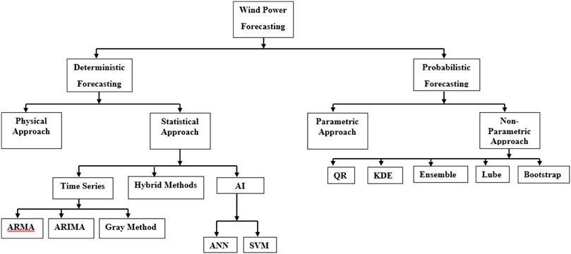
FIGURE 1. Structure of the types of methods used for wind power forecasting (Bazionis and Georgilakis, 2021).

It can be noted from Figure 1 (Bazionis and Georgilakis, 2021) that there exist many related and interconnected methods for solving forecasting problems, but they are mainly categorized into deterministic and probabilistic approaches. Probabilistic forecasting is important not only for energy market operation but also in decision making in power systems for proper power supply.

Spatial–temporal forecasting is recently employed as an interaction between wind parks (Bofinger et al., 2002; Tastu et al., 2014), which focuses on increasing the accuracy of predictions by sharing information from neighboring wind farms as important predictor indicators and tools. Machine learning, deep learning, and artificial intelligence techniques are all being implemented too, which prove to be important future methodologies (Tatsu et al., 2011; Zhang and Wang, 2018). One aspect that has been focused on is ramp events, which pose a threat to power systems as wind power penetrates the global power system more (Cui et al., 2017; Taylor, 2017) due to their dependency on factors such as weather conditions, different time scales, input data accuracy, and multiple nearby locations.

Overall, this approach has shown promising results in improving the accuracy of wind speed forecasting and reducing the associated uncertainty. It has the potential to enhance the performance of wind energy systems, increase energy production, and reduce costs. This work demonstrates how to use a procedural algorithm using measured wind speed data to forecast extracted energy by predicting the shape and scale factors of the Weibull PDF of wind characteristics at the site. As forecasting cannot be predicted accurately, an algorithmized scheme is intended to implement four different methods for future prediction of the wind speed and to estimate any error of each method using four different estimators, as well as a joint probability evaluator of both shape and scale factors to determine variations in the extracted energy forecast.

2 Procedural algorithm

The mean long-term fluctuation of the wind speed is estimated to be within 10%, whereas the short-term fluctuation over the first 4 months of the logged period is more than 20%. The wind direction changes seasonally from southeastern in summer to northwestern in winter. The site wind speed pattern is largely Weibull, with a mean wind speed of around 4 mph. In this work, a combination of deterministic and probabilistic methods is implemented to secure accurate forecasting. The first step of this work is to collect annual wind speed data using a logger. Table 1 lists site data at Fujairah, located NE of the Emirates, on Oman’s gulf coastline.

TABLE 1

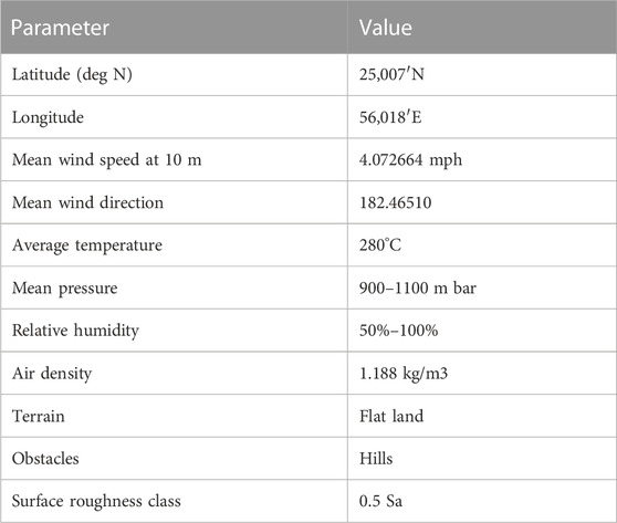
TABLE 1. Wind site characteristics at the Fujairah site.

The annual mean wind speed and direction are measured every 10 s with the wind speed sensor located at 10 m above ground level. Data are logged and recorded together with other meteorological parameters, such as temperature, pressure, humidity, and solar, on the SD card. Figure 2 shows the annual wind speed measured every 10 s, but due to the calm nature of wind speed, signal data were averaged over a day. Hence, less occasionally, sporadic gusts that are blown a few times a year, each lasting for a couple of hours, are eliminated and can be considered noise. It can be noted that wind speed is maximum during the November–March period with maximum fluctuations, whereas much calmer periods are recorded during summer. In general, the site is affected dominantly by western winds in winter and eastern winds in summer.

FIGURE 2

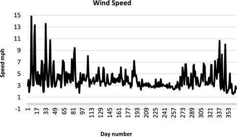
FIGURE 2. Wind speed measurements over a period of 1 year of data. The wind speed is in mph.

The first 11 months starting on 20 February 2020, as day 1, are used for the different methods which are applied for forecasting future wind speed, taken to be month 12, as a reference for comparing the different methods used.

The fluctuating nature of the site wind is highly random and difficult to predict in time and spatial domains, yet by focusing on windy periods, a comparative study is focused on the inherent nature of wind speed and direction. The average annual wind speed is 4.0726 mph, with a maximum speed of 14.8175 mph during this confined period. It can be noticed that the wind speed is concentrated at around 2–5 mph, whereas the wind direction is mostly southern to be in the range of 18^°C–21^°C, with a spike at around 300^°, which is NW in direction. The annual statistics of wind speed measurements are shown in Figure 3 with both a histogram and cumulative histogram.

FIGURE 3

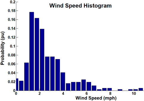
FIGURE 3. Wind speed histogram and cumulative histogram with most variations occurring in the beginning. (MATLAB capture).

Figure 4 demonstrates the procedures that are carried out on measured data to predict the characteristics of the wind speed regime by determining the scale and shape factors of the wind speed Weibull PDF.

FIGURE 4

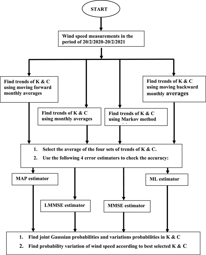
FIGURE 4. Procedural algorithm of methods used in this work.

As shown, four different methods are used to determine the average of the Weibull shape parameter K and Weibull scale parameter C: monthly average, moving forward average, moving backward average, and the Markov series. In addition, four different estimators are used to check for errors in the methods: maximum likelihood estimation (MLE), maximum A posteriori (MAP), minimum mean square error (MMSE), and linear minimum mean square error (LMMSE). Finally, a procedure is implemented to determine the joint Gaussian probability of K and C and variations in their nominal values. It is to declare here that the abovementioned raw wind speed data are duplicated from a previous research work by the author and used as a base foundation for this work here.

Table 2 summarizes the assessment of wind speed residuals, using FFT and wavelet decomposition functions in MATLAB, in which the average values of the synthesized and original signals are found to be equal with the normalized error between them at level 1, found to be 4.9175e-14. The synthesized signal is reconstructed from the decompositions of the original signal, according to wavelet type name and levels.

TABLE 2

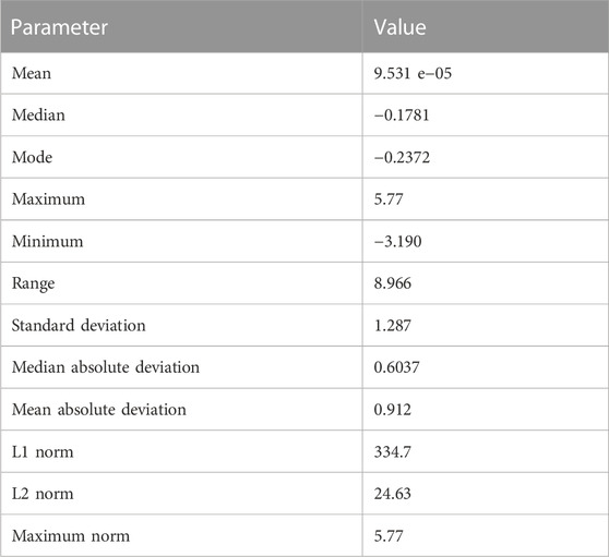
TABLE 2. Wind speed residual assessment.

2.1 Prediction of K and C parameters

Prediction of Weibull PDF factors K and C is determined by invoking several MATLAB functions, such as wblfit (), wblrnd (), wblstat (), and wblplot (),, on the logged data that have been measured over a 1-year period.

2.2 Monthly average

Monthly averages of data are used to find K and C values as depicted in Table 3, in which the first 11 months are used for prediction and month 12 is for checking the prediction. This is plotted in Figure 5 for parameters K and C, respectively, together with the trend curves according to 2^nd-order polynomials relating K and C with the number of months m, and R is the square root error, which is displayed in the plots as well.

TABLE 3

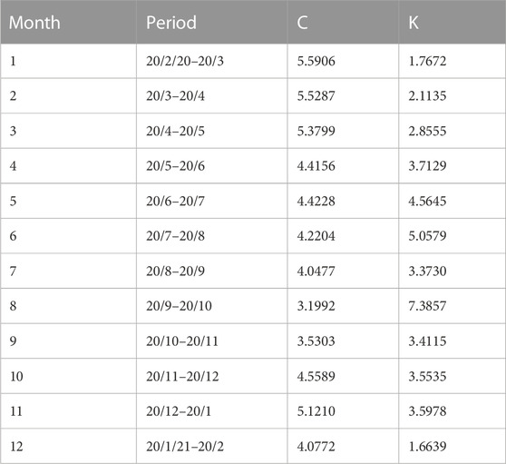
TABLE 3. Wind speed residual assessment.

FIGURE 5

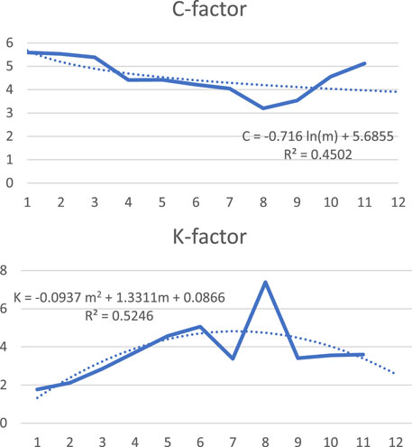
FIGURE 5. Weibull factors K and C evaluated by monthly averages.

It is seen that the forecast for the 12th month is C = 3.95, whereas it is measured to be 4.0772. The error is negligible.

For the K constant, it is forecasted to be 2.4, whereas it is measured to be 1.6639. The error is large and not in line with our expectations due to the abnormal measured value of K in the 12th month, which is not in line with all previous measurements in the first 11 months. From the graph, a value in the range of 2–3 is more appropriate.

2.3 Forward-moving monthly average

In this method, the accumulated averages of the forward-moving months are used for the forecasting of K and C values for the 12th month, to be C = 4.3 and K = 2.3, whereas their values are 4.0772 and 1.6639, respectively. As mentioned, the last measured value of K is not consistent due to the probable sporadic nature of the measured value. Table 4 depicts the monthly measured values of K and C over the first 11 months, with Figure 6 showing the variations of K and C, together with their trends according to 2^nd-order polynomials. It can be noted that in this method, both K and C are nearly constant C, and their expectations are within measured values.

TABLE 4

TABLE 4. Wind speed residual assessment.

FIGURE 6

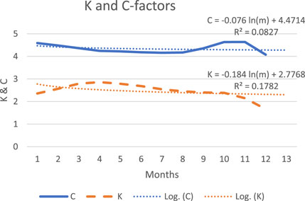
FIGURE 6. Weibull factors K (displayed as a dashed line) and C (displayed as a solid line) with their trends (dotted), evaluated using forward-moving monthly averages.

2.4 Backward-moving monthly average

Similarly, the values of K and C for the first 11 months are listed in Table 5, with their forecasted values for the 12th month to be C = 4.6 and K = 2.4, compared with their measured values for the first 11 months to be 4.5908 and K = 2.3547. Figure 7 displays the variations of both K and C, together with their trends based on the 2^nd-order polynomials. It can be noticed that the error is negligible between the forecasted and measured values, and they vary almost linearly with the months.

TABLE 5

TABLE 5. Wind speed residual assessment.

FIGURE 7

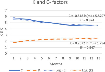
FIGURE 7. Weibull factors K and C evaluated with backward-moving monthly averages.

2.5 Markov series

For the value of factor C of the Weibull PDF, a Markov series is selected with states {3 4 5 6}, which corresponds to percentage probabilities of {0.16 0.22 0.28 0.33}, obtained by rounding the values in Table 3 and then calculating probability percentages. Hence, the following transition probability matrix TM is formed:

$TM=\left[\begin{array}{cc}\begin{array}{cc}0.0& 1.0\end{array}& \begin{array}{cc}0.0& 0.0\end{array}\\ \begin{array}{cc}\begin{array}{c}0.25\\ 0.0\\ 0.0\end{array}& \begin{array}{c}0.0\\ 0.5\\ 0.0\end{array}\end{array}& \begin{array}{cc}\begin{array}{c}0.75\\ 0.5\\ 0.5\end{array}& \begin{array}{c}0.0\\ 0.0\\ 0.5\end{array}\end{array}\end{array}\right],$

and the next states are evaluated to be {0.055 0.3 0.47 0.165}. Therefore, the maximum probability is estimated to be 0.47, corresponding to a value of factor C equal to 5, with the nominal expected total value found to be 4.715 compared with 4.0772. A similar Markov series for the K value is formed with states {2 3 4 5 7} corresponding to percentage probabilities of {0.1 0.14 0.2 0.24 0.3}. Hence, the transition probability matrix is

$TM=\left[\begin{array}{ccc}0.5& 0.5& \begin{array}{ccc}0.0& 0.0& 0.0\end{array}\\ 0.0& 0.5& \begin{array}{ccc}0.25& 0.0& 0.25\end{array}\\ \begin{array}{c}0.0\\ 0.0\\ 0.0\end{array}& \begin{array}{c}0.0\\ 0.5\\ 1.0\end{array}& \begin{array}{ccc}\begin{array}{c}0.0\\ 0.0\\ 0.0\end{array}& \begin{array}{c}1.0\\ 0.5\\ 0.0\end{array}& \begin{array}{c}0.0\\ 0.0\\ 0.0\end{array}\end{array}\end{array}\right],$

with forecasted states {0.05 0.54 0.035 0.32 0.07}, and the maximum probability is 0.54, corresponding to the nominal value of 3, compared with the expected total value of 3.9. It can be noted that forecasting errors are minimum.

3 Estimation errors of the forecasted K and C values

MAP, MLE, MMSE, and LMMSE (Miller and Childers, 2012) will be used here to estimate errors by selecting the most probable value for a given observation. Following the previous four measurements, Table 6 displays the four forecasted values of K and C. Table 7 displays the estimated errors in K and C using the four aforementioned methods.

TABLE 6

TABLE 6. Four forecasted values of K and C.

TABLE 7

TABLE 7. Four forecasted values of K and C.

The observations and detection of K and C values give a correct value plus an error, which is needed to provide their best-estimated values. In this case, it is assumed that for series X = [K₁, K₂, K₃, K₄] or [C₁, C₂, C₃, C₄], there exists value Y to be the maximum likelihood (ML) of either K or C. As previously mentioned in the monthly averages method, the value of measured K is not likely valid, whereas a value between 2 and 3 is more in line within expectation.

3.1.Maximum likelihood

In general, for any length (N) of observations (X), it is required to maximize the conditional PDF of X with Y; $f_{X|Y}$ (x|y). For the MLE, it is assumed that each X is an independent Gaussian random variable with mean Y and variance ${\sigma }_e^2$, and hence, it is possible to determine $f_{X|Y}\left(x,y\right)$ as (Miller and Childers, 2012)

$f_{X|Y}\left(x,y\right)=\frac{1}{{\left(2\pi {\sigma }_e^2\right)}^{\frac{N}{2}}}\exp \left\{-\frac{1}{2{\sigma }_e^2}{\displaystyle \sum _{i=1}^N}{\left(x_i-Y\right)}^2\right\}.(1)$

For the maximum likelihood estimation, Y is modeled to be of a uniform distribution of constant value; i.e., $f_Y\left(y\right)$ does not depend on y since it is constant over all allowable values of y values, and hence, it is needed to maximize only $f_{\mathit{X}|Y}\left(\mathit{x}|y\right)$. That is, there is no prior knowledge about the distribution of Y. Differentiating with respect to y and setting the value equal to zero requires that ${\displaystyle \sum _{i=1}^N}\left(x_i\right.-Y)=0$, and hence, the MLE estimator is given by

$Y_{ML}=\frac{1}{N}{\sum }_{i=1}^N{x}_i,(2)$

which is merely the average value; that is, K_ML = 2.8 and C_ML = 3.4.

$f_{Y|\mathit{X}}\left(y,\mathit{x}\right)=\frac{f_{\mathit{X}|Y}\left(\mathit{x}|y\right)f_Y\left(y\right)}{f_X\left(x\right)}.(3)$

3.2 Maximum A posteriori

It is required to find Y that maximizes $f_{Y|\mathit{X}}\left(y,\mathit{x}\right)$ (Y and X are jointly Gaussian variables of a normal PDF), which can be expressed as

$f_{X|Y}\left(x,y\right)f_Y\left(y\right)=\frac{1}{{\left(2\mathrm{\pi }{\mathrm{\sigma }}_{\mathrm{e}}^2\right)}^{\frac{\mathrm{N}}{2}}}\exp \left\{-\frac{1}{2{\mathrm{\sigma }}_{\mathrm{e}}^2}{\displaystyle \sum _{\mathrm{i}=1}^{\mathrm{N}}}\left({\mathrm{x}}_{\mathrm{i}}\right.-\mathrm{Y}{)}^2\right\}\frac{1}{\sqrt{2\mathrm{\pi }{\mathrm{\sigma }}_{\mathrm{t}}^2}}\exp \left(-\frac{{\left(\mathrm{Y}-{\mathrm{\mu }}_{\mathrm{t}}\right)}^2}{2{\mathrm{\sigma }}_{\mathrm{t}}^2}\right).(4)$

The denominator of (3) is not a function of Y, so it is needed only to maximize the numerator.Differentiating with respect to Y and setting the result equal to zero for maximum value yields the MAP estimator.

$MAP=\frac{\frac{1}{N}{\displaystyle \sum _{i=1}^N}{X}_i+\frac{{\mu }_k{\sigma }_e^2}{N{\sigma }_k^2}}{1+\frac{{\sigma }_e^2}{N{\sigma }_k^2}}.(5)$

It is of note that $\frac{1}{N}{\displaystyle \sum _{i=1}^N}{X}_i$ is the average of all observations. Therefore, the MAP estimator can be considered equal to the average, skewed by prior knowledge of wind speed PDF. In our example, the number of methods used to predict wind speed, N = 4, and μ_K is the mean of measured values, K = 2.8. Assuming a Gaussian variance of K, ${\sigma }_K^2$, to be 20% of the K range = 0.15 and for the Gaussian error, ${\sigma }_e^2$, to be 10% of the nominal value = 0.28, the result obtained is as follows:

$K_{MAP}=\frac{2.8+\frac{2.8\left(0.28\right)}{4\left(0.15\right)}}{1+\frac{0.28}{4\left(0.15\right)}}=2.808.$

Similarly for C, N = 4, μ_C = 3.4, ${\sigma }_c^2=1.4$, and ${\sigma }_e^2=0.34$.

$C_{MAP}=\frac{3.4+\frac{3.4\left(0.34\right)}{4\left(1.4\right)}}{1+\frac{0.34}{4\left(1.4\right)}}=2.244.$

3.3 Minimum mean square error

A third estimation to be used is the MMSE to minimize the square mean error E [(y_i-y_m)^2], where operator E [] is the mean operator, y_i is the true value, and y_m is the estimated value. In our case, the estimated values of K and C are the averages of the four implemented methods as 2.8 and 3.4, respectively.

3.4 Linear minimum mean square error

This estimation is similar to MMSE but with $E[{\left(y_i-y_m\right)}^2$] replaced by $E[{\left(\left\{{a_{1}y}_1+{a_{2}y}_2+{a_{3}y}_3+{a_{4}y}_4\right\}-y_m\right)}^2$], which leads to

$y_{LMMSE}=\frac{\frac{1}{N}{\displaystyle \sum _{i=1}^N}{y}_i}{1+\frac{{\sigma }_e^2}{\left({\sigma }_t^2+{\mu }_t^2\right)N}}.(6)$

Substituting the same values used in MAP, i.e., N = 4, μ_K is the mean of measured values of K = 2.8. The Gaussian variance of K, ${\sigma }_k^2$, is assumed to be 20% of the K range = 0.15 (ignoring the last value), and the Gaussian error, ${\sigma }_e^2$, is assumed to be 10% of the nominal value = 0.28. Hence,

$K_{LMMSE}=\frac{\frac{1}{N}{\displaystyle \sum _{i=1}^N}{K}_i=2.8}{1+\frac{{0.28}^2}{\left(0{.15}^2+{2.8}^2\right)4}}=2.8.$

Similarly for C, N = 4, μ_C = 3.4, ${\sigma }_c^2=1.4$, and ${\sigma }_e^2=0.34$.

$C_{LMMSE}=\frac{\frac{1}{N}{\displaystyle \sum _{i=1}^N}{C}_i=3.4}{1+\frac{{0.34}^2}{\left({1.4}^2+{3.4}^2\right)4}}=3.4.$

It can be deduced that the estimated values of K and C using the four different types of estimation are indeed within the range of their evaluations by the four implemented methods.

4 Prediction of the joint probability of K and C

The probability of wind speed occurrence P (as a percentage of hours/year per mph) is normally expressed by the Weibull distribution function (Hodge, 2010) as

$P\left(v,k,c\right)=\frac{K}{C}{\left(\frac{v}{C}\right)}^{K-1}\mathit{exp}\left[-{\left(\raisebox{1ex}{$v$}\!\left/ \!\raisebox{-1ex}{$c$}\right.\right)}^K\right].(7)$

As the logged wind speed resembles a sharp Weibull pattern, a value of K is chosen. The scale parameter C can be estimated by integrating (7) over the whole range of wind speeds.

$V_{mean}={\displaystyle \underset{0}{\overset{\infty }{\int }}}v\frac{K}{C}{\left(\frac{v}{C}\right)}^{K-1}\mathit{exp}\left[-{\left(\frac{v}{C}\right)}^K\right]dv.(8)$

It can be assumed that both K and C are defined each with a value plus an error that is modeled as a Gaussian random variable with zero mean and with a defined variance, and hence, they themselves are Gaussian variables with a PDF equal to

$f_X\left(x\right)=\frac{1}{\sqrt{2\pi {\sigma }^2}}\exp \left(-\frac{{\left(x-m\right)}^2}{2{\sigma }^2}\right).(9)$

Substituting values related to K and C from previous interpretations, with mean values of 2.6 and 3.95 and variances of approximately ${\sigma }_k=0.2$ and ${\sigma }_c=0.7$, respectively, yields

$f_K\left(k\right)=\frac{1}{\sqrt{2\pi {\left(0.2\right)}^2}}\mathit{exp}\left(-\frac{{\left(K-1.2\right)}^2}{2{\left(0.2\right)}^2}\right)=2e^{-12.5{\left(K-1.2\right)}^2},(10)$

$f_C\left(c\right)=\frac{1}{\sqrt{2\pi {\left(0.7\right)}^2}}\mathit{exp}\left(-\frac{{\left(C-2.2\right)}^2}{2{\left(0.7\right)}^2}\right)=0.57e^{-{\left(C-2.2\right)}^2}.(11)$

On the other hand, the joint probability of N independent the PDF’s $f_{X_n}$ for $\mathit{X}$ random variables is expressed as

$f_{\mathit{X}}\left(\mathit{x}\right)={\displaystyle \prod _{n=1}^N}{f}_{X_n}\left(x_n\right).(12)$

Hence, for random variables K and C, it yields

$f_{K,C}\left(k,c\right)=f_K\left(k\right)f_C\left(c\right).(13)$

K and C are correlated with some correlation factor ρ; hence, (13) is modified with an assumed value of ${\rho }_{kc}$ = 0.5 into

$f_{K,C}\left(k,c\right)=\frac{1}{2\pi {\sigma }_k{\sigma }_c\sqrt{1-{\rho }_{kc}^2}}\mathit{exp}\left(\frac{{\left(\frac{K-{\mu }_k}{{\sigma }_k}\right)}^2-2\rho \left(\frac{K-{\mu }_k}{{\sigma }_k}\right)\left(\frac{C-{\mu }_c}{{\sigma }_c}\right)+{\left(\frac{C-{\mu }_c}{{\sigma }_c}\right)}^2}{2\left(1-{\rho }^2\right)}\right),(14)$

and substituting the mean and variance values of K and C leads to$f_{K,C}\left(k,c\right)=.069e^{-\left\{0.96{\left(K-.2\right)}^2-0.252\left(K-.2\right)\left(C-.7\right)+0.302{\left(C-.7\right)}^2\right\}}$. It is of note that

$f_{K,C}\left(k,c\right)=f_{K|C}\left(k|c\right)f_C\left(c\right)=f_{C|K}\left(c|k\right)f_K\left(k\right).(15)$

It would be useful here to check variations in the probability of wind speed in the response of any variation in C according to its Gaussian PDF (Miller and Childers, 2012). Hence, $f_{\mathit{V}}\left(\mathit{v}\right)=f_{V|C}\left(v|c\right)f_C\left(c\right)$, which can be reduced to

$f_{\mathit{V}}\left(\mathit{v}\right)=\frac{K}{C}{\left(\frac{v}{C}\right)}^{K-1}{e}^{{}^{\left[-{\left(\raisebox{1ex}{$v$}\!\left/ \!\raisebox{-1ex}{$C$}\right.\right)}^K\right]}}\left\{0.57e^{-{\left(C-2.2\right)}^2}\right\}.(16)$

Figure 8 depicts probabilities of wind speed at different values of scale factor C, when it is varied by ± 20% around its Gaussian PDF nominal mean with a range of values of 2–4, keeping the shape factor K constant, since variations of scale factor are more dominant than the shape factor (Majid, 2021). When the variation of the Weibull shape factor K is inconsistent, then the joint probability depicted in (14) should be used, since determining both factors as accurately as possible is important to forecast wind speed probability and, hence, the extracted wind energy.

FIGURE 8

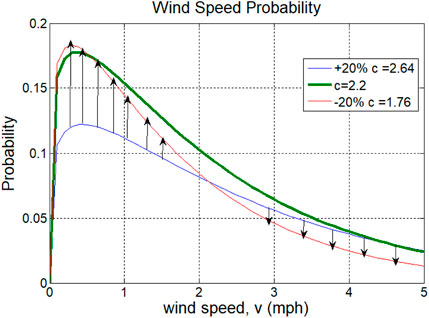
FIGURE 8. Probability of wind speed due to variations in the scale factors of the wind speed Weibull PDF.

5 Conclusion

An algorithm was proposed to estimate the scale and shape parameters of the Weibull probability density function (PDF) that characterizes the wind regime at the Fujairah site. This was performed by averaging the results from four simulation methods. To evaluate the accuracy of the analysis, different error estimation techniques, such as ML, MAP, MMSE, and LMMSE, were employed. The accuracy of the analysis was verified using the Markov series method. To predict the effects of variations in the Weibull PDF scale factor on wind speed forecasting and wind energy production, a detailed joint probability analysis was conducted. It was observed that a 20% variation in the Weibull PDF scale factor has a significant impact on wind speed forecasting. Therefore, this factor was identified as the major factor to be varied.

Data availability statement

The raw data supporting the conclusion of this article will be made available by the author, without undue reservation.

Author contributions

The author confirms being the sole contributor of this work and has approved it for publication.

Conflict of interest

The author declares that the research was conducted in the absence of any commercial or financial relationships that could be construed as a potential conflict of interest.

Publisher’s note

All claims expressed in this article are solely those of the authors and do not necessarily represent those of their affiliated organizations, or those of the publisher, the editors, and the reviewers. Any product that may be evaluated in this article, or claim that may be made by its manufacturer, is not guaranteed or endorsed by the publisher.

Supplementary material

The Supplementary Material for this article can be found online at: https://www.frontiersin.org/articles/10.3389/fenrg.2023.1194010/full#supplementary-material

References

Bazionis, I. K., and Georgilakis, P. S. (2021). Review of deterministic and probabilistic wind power forecasting: models, methods, and future research. Electricity 2, 13–47. doi:10.3390/electricity2010002

CrossRef Full Text | Google Scholar

Bofinger, S., Luig, A., and Beyer, H. (2002). “Qualification of wind power forecasts,” in Proceedings of the global wind power conference (Paris, France.

Google Scholar

Cui, M., Zhang, J., Wang, Q., Krishnan, V., and Hodge, B. M. (2017). A data-driven methodology for probabilistic wind power ramp forecasting. IEEE Trans. Smart Grid 10, 1326–1338. doi:10.1109/tsg.2017.2763827

CrossRef Full Text | Google Scholar

Foley, A. M., Leahy, P. G., Marvuglia, A., and McKeogh, E. I. (2012). Current methods and advances in forecasting of wind power generation. Renew. Energy 37, 1–8. doi:10.1016/j.renene.2011.05.033

CrossRef Full Text | Google Scholar

Giebel, G., Brownsword, R., Kariniotakis, G., Denhart, M., and Draxl, C. “The state-of-the-art in short-term prediction of wind power,” in A literature overview. 2nd Ed. Online. Available at: https://orbit.dtu.dk/en/publications/the-state-of-the-art-in-short-term-prediction-of-wind-power-a-lit (accessed October 10, 2020).

Google Scholar

Hodge, B. K. (2010). “Wind energy,” in Alternative energy Systems and applications, a book (John Wiley), 56–87. ISBN: 978-0-470-14250-9.

Google Scholar

Hodge, B., and Milligan, M. (2011). “Wind power forecasting error distributions over multiple timescales,” in Proceedings of the IEEE power and (Detroit, MI, USA: Energy Society General Meeting).

CrossRef Full Text | Google Scholar

Jabr, R. (2013). Adjustable robust OPF with renewable energy sources. IEEE Trans. Power Syst. 28, 4742–4751. doi:10.1109/tpwrs.2013.2275013

CrossRef Full Text | Google Scholar

Jung, J., and Broadwater, R. P. (2014). Current status and future advances for wind speed and power forecasting. Renew. Sustain. Energy Rev. 31, 762–777. doi:10.1016/j.rser.2013.12.054

CrossRef Full Text | Google Scholar

Lei, M., Shiyan, L., Chuanwe, J., Hongling, L., and Yan, Z. (2009). A review on the forecasting of wind speed and generated power. Renew. Sustain. Energy Rev. 13, 915–920. doi:10.1016/j.rser.2008.02.002

CrossRef Full Text | Google Scholar

Majid, A. (2021). The evaluation of wind energy based on the inherent nature of wind speed assessment at Fujairah (UAE). Instrum. Mes. Métrologie 20 (3), 121–130. doi:10.18280/i2m.200301

CrossRef Full Text | Google Scholar

Miller, S., and Childers, D. (2012). “Multiple random variables,” in Probability and random processes with applications to signal processing and communications. a book, AP, ISBN: 978-0-12-386981-4.

Google Scholar

Pinson, P., Chevallier, C., and Kariniotakis, G. (2007). Trading wind generation from short-term probabilistic forecasts of wind power. IEEE Trans. Power Syst. 22, 1148–1156. doi:10.1109/tpwrs.2007.901117

CrossRef Full Text | Google Scholar

Pinson, P. (2012). Very short-term probabilistic forecasting of wind power with generalized logit-normal distributions. J. R. Stat. Soc. Ser. C 61, 555–576. doi:10.1111/j.1467-9876.2011.01026.x

CrossRef Full Text | Google Scholar

Soman, S. S., Zareipour, H., Malik, O., and Mandal, P. (2010). “A review of wind power and wind speed forecasting methods with different time horizons,” in Proceedings of the north American power symposium (Arlington, TX, USA.

CrossRef Full Text | Google Scholar

Tastu, J., Pinson, P., Trombe, P., and Madsen, H. (2014). Probabilistic forecasts of wind power generation accounting for geographically dispersed information. IEEE Trans. Smart Grid 5, 480–489. doi:10.1109/tsg.2013.2277585

CrossRef Full Text | Google Scholar

Tatsu, J., Pinson, P., Kotwa, E., Madsen, H., and Nielsen, H. A. (2011). Spatio-temporal analysis and modeling of short-term wind power forecast errors. Wind Energy 14, 43–60. doi:10.1002/we.401

CrossRef Full Text | Google Scholar

Taylor, J. (2017). Probabilistic forecasting of wind power ramp events using autoregressive logit models. Eur. J. Oper. Res. 259, 703–712. doi:10.1016/j.ejor.2016.10.041

CrossRef Full Text | Google Scholar

Wang, Q., Guan, Y., and Wang, J. (2012a). A chance-constrained two-stage stochastic program for unit commitment with uncertain wind power output. IEEE Trans. Power Syst. 27, 206–215. doi:10.1109/tpwrs.2011.2159522

CrossRef Full Text | Google Scholar

Wang, X., Guo, P., and Huang, X. (2012b). A Review of wind power forecasting models. Energy Procedia 12, 770–778. doi:10.1016/j.egypro.2011.10.103

CrossRef Full Text | Google Scholar

Wu, Y. K., Po, E. S., and Jing, S. H. (2016). “An overview of wind power probabilistic forecasts,” in Proceedings of the IEEE PES asia-pacific power and energy engineering conference (China: Xi’an).

CrossRef Full Text | Google Scholar

Yan, J., Liu, Y., Han, S., Wang, Y., and Feng, S. (2015). Reviews on uncertainty analysis of wind power forecasting. Renew. Sustain. Energy Rev. 52, 1322–1330. doi:10.1016/j.rser.2015.07.197

CrossRef Full Text | Google Scholar

Zhang, Y., and Wang, J. A. (2018). A distributed approach for wind power probabilistic forecasting considering spatio-temporal correlation without direct access to off-site information. IEEE Trans. Power Syst. 33, 5714–5726. doi:10.1109/tpwrs.2018.2822784

CrossRef Full Text | Google Scholar

Zhang, Y., Wang, J., and Wang, X. (2014). Review on probabilistic forecasting of wind power generation. Renew. Sustain. Energy Rev. 32, 255–270. doi:10.1016/j.rser.2014.01.033

CrossRef Full Text | Google Scholar

Zhang, Z., Sun, Y., Gao, D., Lin, J., and Cheng, L. (2013). A Versatile probability distribution model for wind power forecast errors and its application in economic dispatch. IEEE Trans. Power Syst. 28, 3114–3125. doi:10.1109/tpwrs.2013.2249596

CrossRef Full Text | Google Scholar