 Xian Xu
 Yingchun Chen
- Shanghai Aircraft Design and Research Institute, Shanghai, China
In this paper, an adaptive mesh refinement technique is presented for simulation of compressible flows, which can effectively refine the mesh in the regions with shock waves and vortices. The present approach uses the total energy per unit volume as an indicator to capture the shock waves and vortical structures. In the approach, an h-refinement strategy is adopted. To save the computational effort, the flow variables on the new mesh are obtained from the previous step by interpolation, which ensures that the problem is always solved on the refined mesh. Both inviscid and viscous compressible flows are considered in this work. Their governing equations are, respectively, Euler equations and Navier–Stokes equations associated with the implementation of the Spalart–Allmaras turbulence model. The cell-centered finite volume method and Jameson scheme are chosen to carry out spatial discretization, and the five-stage Runge–Kutta scheme is applied to discretize the temporal derivative. The present approach is applied to simulate three test problems for its validation. Numerical results show that it can effectively capture the shock waves and vortices with improvement in solution accuracy.
1 Introduction
To analyze the fluid characteristics, accurate simulation of the flow field is one of the main tasks in computational fluid dynamics (CFD). A high-quality mesh plays an important role in solution accuracy of the flow field. Generation of a good mesh usually requires some prior knowledge of the flow behavior in order to match the mesh point distribution to the essential features of the flow field. However, this prior knowledge may not always be available in advance. On the other hand, if the mesh is refined in the whole domain to guarantee the desired solution accuracy, the amount of computational time, effort, and resources may become excessive. How to balance the high-quality mesh and the computational effort is a critical issue. It seems that the solution-adaptive mesh refinement technique is an answer to this problem. It can effectively refine the mesh only in pivotal regions to improve the solution accuracy. In fact, research on this aspect is currently a hot topic in CFD (Harvey et al., 1992; Murayama et al., 2001; Yamazaki et al., 2007; Fossati et al., 2010).
One of the key issues in the solution-adaptive mesh refinement process is the identification of cells for refinement. Much effort has been devoted to this part (Murayama et al., 2001; Aftosmis and Berger, 2002; Jones et al., 2006; Yamazaki et al., 2007). The parameter used to identify the mesh refinement is generally called an adaptation function or indicator. Usually, the adaptation function is associated with some key physical variables such as density, entropy, kinetic energy, or a combination of them (Peraire et al., 1987). Some physical variables, such as helicity density and turbulent kinetic viscosity, are not always easy to derive, and the form of adaptation function may be complicated (Fossati et al., 2010). Under the premise of compressible flows, most adaptation functions are designed to resolve either shock waves or vortices (Pirzadeh, 1999; Ito et al., 2009). As the features of shock waves (high gradients for pressure and density) are quite different from those of vortices (high velocity gradients), a single adaptation function for compressible flows can usually only detect one feature of them. Wang et al. (2020) utilized adaptive mesh refinement (AMR) to capture vortices for improving the accuracy and efficiency of numerical simulation of the cavitation–vortex interaction. Steinthorsson et al. (1994) introduced a methodology based on the AMR algorithm of Berger and Colella (1989) for the accurate and efficient simulation of unsteady, compressible flows. Gou et al. (2018) introduced an accurate and robust AMR system suitable for turbomachinery applications and widely studied shock wave and tip leakage using the AMR method. Pantano et al. (2007) presented a methodology for the large-eddy simulation of compressible flows with a low-numerical dissipation scheme and structured adaptive mesh refinement (SAMR) used in turbulent flow regions while employing weighted essentially non-oscillatory order (WENO) to capture shocks. Papoutsakis et al. (2018) presented an adaptive mesh refinement (AMR) method suitable for hybrid unstructured meshes that allows for local refinement and de-refinement of the computational grid during the evolution of the flow to increase the order of accuracy in the region of shear layers and vortices. This paper takes this challenging issue and aims to present an indicator which can well detect both the shock waves and vortices in the compressible flow using h-type AMR.
This paper is organized as follows: in Section 2, the governing equations and methodologies for numerical discretization are briefly described. Section 3 depicts the solution-adaptive mesh refinement approach which involves the selection of the adaptation function and the h-refinement strategy (Pepper and Wang, 2007) based on body-fitted quadrilateral/hexahedral mesh. Section 4 presents three numerical examples to validate the present approach. We report conclusion in Section 5.
2 Governing equations and numerical discretization
The viscous, compressible flow of a perfect gas is governed by Navier–Stokes (N–S) equations (Blazek, 2001a). In a three-dimensional domain of volume
Here,
where
where
The total enthalpy
where
are the terms describing the work of viscous stresses and the heat conduction in the fluid.
Here, cp is the specific heat coefficient at constant pressure,
Generally, both
In this work, the Spalart–Allmaras (S–A) one-equation turbulence model (Spalart and Allmaras, 1992) is adopted. In this model, a transport equation is employed to calculate an eddy-viscosity variable
Here,
The terms controlling the destruction of the eddy viscosity read
and the production term
Here,
Finally, the constants in Eqs 8–10 are defined as
In current simulation,
When the ideal gas is considered, we can simply neglect the viscous effect and get rid of
To spatially discretize the governing equations, the finite volume method (FVM) is used in this study. FVM first divides the physical space into a number of control volumes and then integrates the governing equation (Eq. 1) over each control volume. In this work, the Jameson cell-centered scheme (Jameson et al., 1981) is used to define the location and shape of the control volume. The mean theorem is applied to approximate both the volume integral and the surface integral. The surface integral involves evaluation of fluxes at the interface between two neighboring control volumes. The flow quantities are stored at the centroids of each control volume which coincides with the grid cell. Note that with the mean theorem, the convective and the viscous fluxes are only evaluated at the center of each control surface using the flow information adjacent to two sides of the interface.
Two-dimensional grid is taken as an example. Using the cell-centered finite volume approach, in which the conserved variables
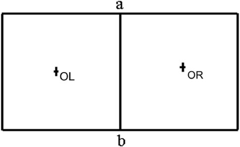
FIGURE 1. Cell-centered scheme of Jameson.
Cell-centered schemes such as the one described previously would lead to odd–even decoupling of the solution, so that any errors are not damped and oscillations will be presented in the steady-state solution. Artificial dissipation terms
where the index
where
Adaptive coefficients
where
where c and
After spatial discretization, the resultant ordinary differential equations can be solved using the explicit five-stage Runge–Kutta scheme of Jameson et al. (1981).
where
3 Total energy-based adaptive mesh refinement approach
3.1 Selection of total energy per unit volume as the refinement indicator
After obtaining the basic solution of governing equations in the flow field, two important steps in any solution-adaptive mesh refinement technique must be followed. The first one requires an indicator to detect and locate the flow structures of interest, where the mesh refinement is needed. From a practical point of view, the adaptation function should indicate where the mesh must be refined to improve the accuracy. The adaptation function is usually selected from flow variables such as density, entropy, and turbulent kinetic energy. The flow considered in this paper is at high Reynolds number, and the Mach number ranges from low-compressible regime (Mach number < 0.3) to supersonic regime (Mach number > 1.0). In some cases, the viscous effect is very important. Thus, there is a practical demanding to select an adaptation function which can well capture both the features of shock waves and viscous effect.
It is known that any perturbation of flow must be followed by the perturbation of total energy per unit volume (
where subscripts
The summation is only performed for cells which satisfy
In the refinement process, the value of
3.2 Mesh refinement process
After determining the indicator, the process of mesh refinement, as the second step in adaptive technique, can be executed. In general, adaptive methods can be roughly classified into three categories (Pirzadeh, 2000; Pepper and Wang, 2007): grid movement (r-refinement), grid enrichment (h-refinement), and local solution enhancement (p-refinement). Each method has its own merits and shortcomings (Pepper and Wang, 2007; Li et al., 2010).
In the r-refinement method, the value of the adaptation function directly determines the mesh spacing. As described previously, the values of adaptation function in this work do not represent the magnitudes of estimated errors. Instead, they only indicate the location of dominant flow features. Therefore, r-refinement is not appropriate for this work. At the same time, although the p-refinement approach can obtain a solution with high order of accuracy in smooth flow regions, it is not effective in regions with discontinuity of flow variables. In addition, the coding of p-refinement is very complicated. In the methods based on h-refinement, however, an adaptation function only serves as a means to locate the regions which can be refined without considering the mesh spacing. Additionally, the h-refinement approach can be effectively applied in both the smooth flow and discontinuous flow regions. Due to these advantages, the h-refinement process is adopted in this work.
To reduce the number of cells, and in the meantime, to well capture the thin boundary layer, the structured mesh is taken as the background mesh. Grid cells are quadrilaterals for two-dimensional cases and hexahedra for three-dimensional cases. It should be indicated that as refinement process goes on, the overall unstructured mesh is formed.
During refinement, each quadrilateral/hexahedron is divided into four/eight sub-cells by joining the midpoints of opposite faces, as shown in Figure 2. For the two-dimensional case, to the initial coarse grid cell, a parent face is replaced by the current parent face and a new child face. This may form a hanging node (Spragle et al., 1995) between the initial coarse cell and the refined cells.
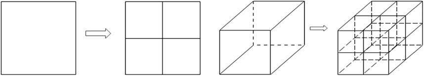
FIGURE 2. Refinement strategies.
A node is a hanging node if it is not a vertex of all cells sharing one face. The hanging node grid adaptive scheme has the ability to efficiently operate on grids with a variety of cell shapes, including hybrid grids. However, the hanging node adaption scheme makes some solvers unusable, especially for the structured solvers. In contrast, the face-based unstructured solver presented by Li et al. (2010) provides an ideal environment for dealing with a hanging node adaption scheme. For the cell-centered scheme used in this work, as shown in Figure 1, the solver simply visits each face and then uses flow variables on its left and right grid cell to evaluate the face flux, and the contribution of the face flux is then sent to the two neighboring cells sharing the interface.
Once the integration loop is performed along all face indexes, spatial discretization of the governing equations is completed.
To maintain a smooth variation of cell volume, additional cells are refined based on the relative position of neighboring cells or boundary conditions. There are three cases shown in Figure 3 in which cell M must be refined. One is that a cell has only one neighboring cell which is refined but its opposing neighboring cell is the solid wall (Figures 3A, D). The second is that a cell has two opposing neighboring cells (Figures 3B, E) or more than two neighboring cells are refined. If the initial grid needs more than one adaptation, then the third case (Figure 3C) arises: a cell has a neighboring cell which has two or more levels. For these cases, additional refinement is needed.
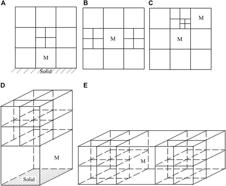
FIGURE 3. Unsmooth cells. (A) A two-dimensional cell has only one adaptive neighboring cell and its opposing neighboring cell is the wall. (B) A two-dimensional cell has two opposing adaptive neighboring cells. (C) A two-dimensional cell has a neighboring cell which has two or more adaptive levels. (D) A three-dimensional cell has only one adaptive neighboring cell and its opposing neighboring cell is the wall. (E) A three-dimensional cell has two opposing adaptive neighboring cells.
The flow field variables of new children cells can be interpolated from their parent cells. To carry out that, there are several different techniques. The simplest way, which is employed in this work, is to directly copy all physical variables of parent cells to their children cells. Such kind of implementation can improve the computational efficiency.
The process of the refinement strategy is summarized in the flowchart as shown in Figure 4. On the other hand, it should be noted that the coarsening process, which is not required in this paper, can be easily implemented based on the obtained information during the refinement process.
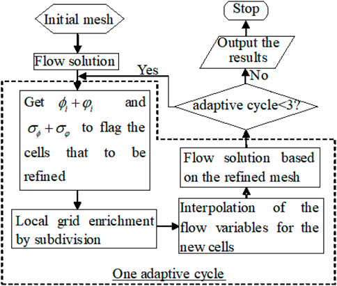
FIGURE 4. Flowchart of the process of the refinement strategy.
4 Numerical examples
To validate the present approach and demonstrate its capability for effective simulation of inviscid/viscous compressible flows, three typical problems are selected. The first problem is a two-dimensional inviscid flow in a channel with a 15° ramp with the typical multi-channel shock wave and expansion wave, to demonstrate the capability to capture shock waves. The second problem is the three-dimensional inviscid flow around the ONERA M6 wing at a transonic speed resulting in a λ shock wave on the upper surface of the wing, to show the capability of the algorithm to capture shock waves in a transonic flow. In the third problem, we hope to show the capability of the algorithm on simulating a detached vortex of a delta wing, especially the vortex core fragmentation, which is important in calculating the lift and drag coefficients.
4.1 Two-dimensional inviscid flow in a channel with a ramp
By solving Euler equations, the results for supersonic flow at a Mach number of 2 in a channel with a
The initial mesh is a uniform mesh containing
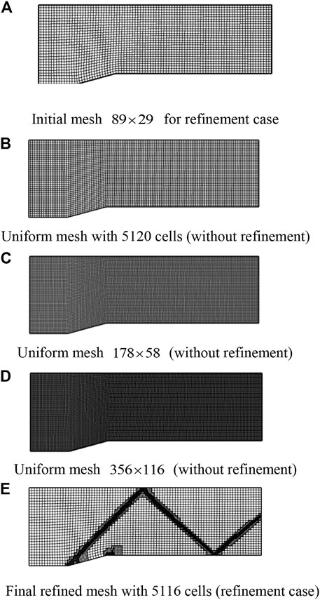
FIGURE 5. Uniform meshes and final refined mesh after two levels of adaptation. (A) Initial mesh
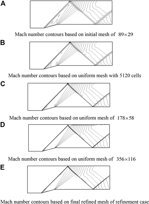
FIGURE 6. Mach number contours in the contracted channel based on uniform meshes and final refined mesh. (A) Mach number contours based on the initial mesh of
To compare the computational cost (cells and seconds) between cases with refinement and without refinement, numerical simulation of the same problem on the three uniform meshes without refinement is carried out. The three uniform meshes without refinement are shown in Figures 5B–D. The mesh in Figure 5B has 5,120 cells. The number of cells for this mesh is the same as the final refined mesh of the refinement case. The mesh in Figure 5C has 10,324 cells which are approximately two times the cells in the final refined mesh of the refinement case. The mesh spacing for this case is the same as the minimum mesh spacing of the refinement case when the initial mesh shown in Figure 5A is refined by one adaption level. The mesh in Figure 5D has 41,296 cells which are approximately eight times the cells in the final refined mesh of the refinement case. The mesh spacing for this case is the same as the minimum mesh spacing of the refinement case when the initial mesh in Figure 5A is refined by two adaption levels. All the results (Mach number contour) are demonstrated in Figure 6. The minimum and maximum levels of contours are 1.0 and 1.8 respectively, and the number of levels is 14. Figures 6A–D show that the shock wave becomes thinner and thinner with the increase in cell numbers. It is seen clear from the figure that the results of the uniform mesh of 41,296 cells are very close to those of the final refined mesh where two adaption levels are used to refine the mesh. This can be well understood as both cases have the same mesh spacing in the vicinity of the shock wave. The computational time required on the meshes shown in Figure 5 is listed in Table 1. It can be observed from Table 1 that the refinement case with two adaption levels only takes approximately 10% of the computational time of the uniform mesh case (without refinement) when the mesh spacing near the shock wave is kept the same. This well demonstrates high computational efficiency of the solution-adaptive approach.
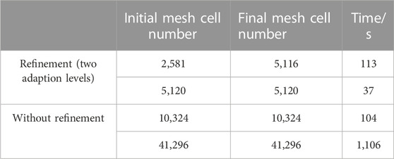
TABLE 1. Comparison of computational cost among different meshes.
4.2 Three-dimensional inviscid flow around the ONERA M6 wing
To further demonstrate the capability of the present solution-adaptive mesh refinement approach for capturing the shock wave, the inviscid flow around the ONERA M6 wing is considered. The Mach number is 0.84, and the incidence is 3.06°. Same as the case in Section 4.1, the governing equations are Euler equations.
A background mesh with a nearly uniform grid distribution is generated as shown in Figure 7A. The initial mesh contains 294,912 hexahedral cells. Figure 7B shows the final refined mesh which contains 440,365 hexahedral cells. Obviously, the majority of mesh refinement occurs in the shock wave regions, and the refined cells clearly outline the
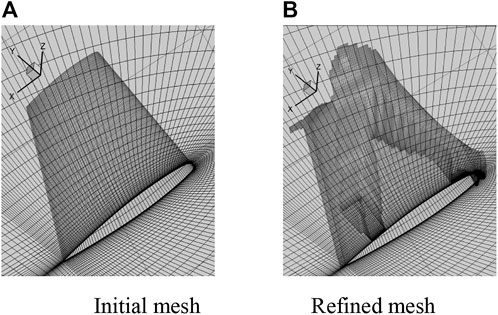
FIGURE 7. Initial and refined mesh for the ONERA M6 wing. (A) Initial mesh. (B) Refined mesh.
The surface pressure coefficient distributions at 0.65 and 0.8 spanwise locations obtained on the initial coarse mesh and the final refined mesh are compared in Figure 8 with the experimental data (Schmitt and Charpin, 1979). The comparison indicates that the shock wave is diffused due to the coarse mesh. The high resolution of shock waves by the refined mesh is evident as revealed by sharp discontinuity of the pressure distribution. There are some deviations between the numerical results and the experimental data. The reason may be due to the fact that the inviscid flow is assumed in the numerical computation, while the real flow always involves viscous effect.
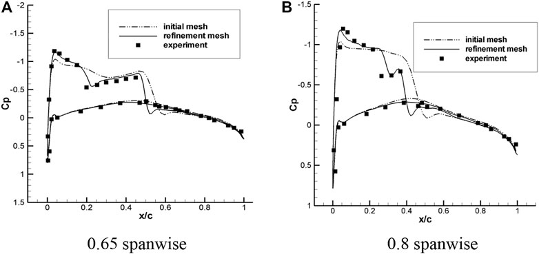
FIGURE 8. Pressure coefficient distributions at 0.65 and 0.8 spanwise locations for the ONERA M6 wing. (A) 0.65 spanwise. (B) 0.8 spanwise.
Numerical simulations for two-dimensional inviscid flows in a channel with a ramp and three-dimensional inviscid flows around the ONERA M6 wing well demonstrate the capability of the present solution-adaptive mesh refinement approach for capturing shock waves and expansion waves. To illustrate the ability of the present approach for capturing vortices, numerical simulation of three-dimensional compressible viscous flows around a delta wing is considered in the following example. The prediction of leading-edge vortex breakdown on a delta wing at high angles of attack is made.
4.3 Three-dimensional viscous flow around a delta wing
The geometry chosen for this case is a flat-plate semispan delta wing with a leading-edge sweep of
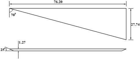
FIGURE 9. Flat-plate semispan delta wing model.
The initial mesh and the adaptive refined mesh are displayed in Figure 10. The corresponding adaptation function is shown in Figure 11. The initial mesh contains 320,624 hexahedral cells. After refinement, the final mesh contains 503,317 hexahedral cells.
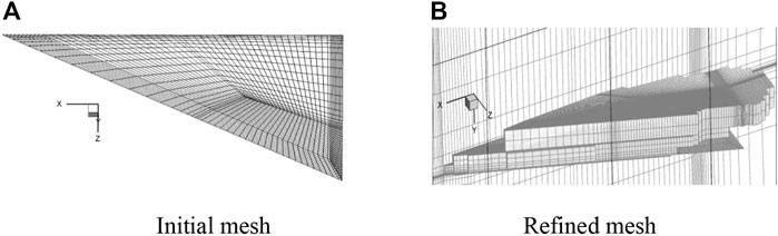
FIGURE 10. Initial mesh and refined mesh for the delta wing. (A) Initial mesh. (B) Refined mesh.
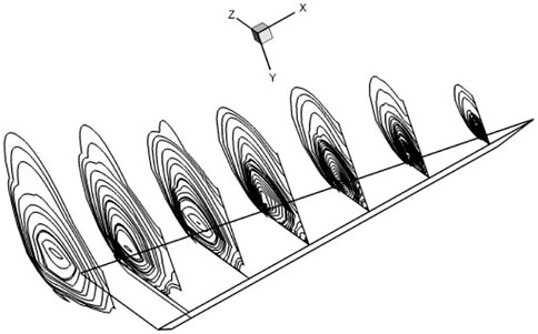
FIGURE 11. Contours of
Figure 12 shows some numerical results for this problem. The solution presented in Figure 12A shows the vortex core line without vortex breakdown, which is different from the solution based on the refined mesh presented in Figure 12B.
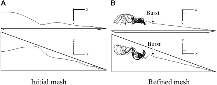
FIGURE 12. Vortex breakdown position indicated by the core line,
5 Conclusion
A solution-adaptive mesh refinement technique, which is based on the total energy per unit volume as the refinement indicator, is presented in this work. Different from previous adaptation indicator used, the present indicator can well detect both the shock waves and vortices. The technique is validated by applying it to simulate two-dimensional and three-dimensional steady compressible inviscid/viscous flows. The h-refinement approach by subdivision is adopted to perform the mesh refinement process.
The capability of the present solver is verified by applying it to handle three test problems. For inviscid/viscous flows, the Euler/Navier–Stokes (with the Spalart–Allmaras one-equation turbulence model) equations are employed. The cell-centered finite volume method is applied for spatial discretization, and an explicit five-stage Runge–Kutta scheme is used to implement time integration. Numerical results show that the proposed adaptation function can well capture the shock waves, expansion waves, and vortices in the flow field. As a consequence, a high-resolution solution of important flow features such as shock waves and vortices is obtained.
Data availability statement
The original contributions presented in the study are included in the article/Supplementary Material; further inquiries can be directed to the corresponding author.
Author contributions
Conceptualization and methodology, XX; methodology, YC; resources and data curation, ZH; writing—original draft preparation, XX; writing—review and editing, ZH; supervision, FZ; project administration, XX; funding acquisition, YC. All authors listed have made a substantial, direct, and intellectual contribution to the work and approved it for publication.
Funding
This research was funded by the National Key R&D Program of China (Project No. 2020YFA0712000).
Conflict of interest
The authors declare that the research was conducted in the absence of any commercial or financial relationships that could be construed as a potential conflict of interest.
Publisher’s note
All claims expressed in this article are solely those of the authors and do not necessarily represent those of their affiliated organizations, or those of the publisher, the editors, and the reviewers. Any product that may be evaluated in this article, or claim that may be made by its manufacturer, is not guaranteed or endorsed by the publisher.
References
Aftosmis, M. J., and Berger, M. J. “Multilevel error estimation and adaptive h-refinement for Cartesian meshes with embedded boundaries,” in Proceedings of the 40th AIAA Aerospace Sciences Meeting & Exhibit, Reno, NV, USA, January 2002. doi:10.2514/6.2002-863
Agrawal, S., Barnett, R. M., and Robinson, B. A. (1992). Numerical investigation of vortex breakdown on a delta wing. AIAA J. 30 (3), 584–591. doi:10.2514/3.10960
Berger, M. J., and Colella, P. (1989). Local adaptive mesh refinement for shock hydrodynamics. J. Comput. Phys. 82 (1), 64–84. doi:10.1016/0021-9991(89)90035-1
Blazek, J. (2001). Computational fluid dynamics: Principles and applications. Kidlington, England: Elsevier Science Ltd, 5–22.
Blazek, J. (2001). Computational fluid dynamics: Principles and applications. Kidlington, England: Elsevier Science Ltd, 225–265.
Fossati, M., Guardone, A., and Vigevano, L. (2010). A node-pair finite element/finite volume mesh adaptation technique for compressible flows. Int. J. Numer. Methods Fluids 70. doi:10.1002/fld.2728
Gou, J., Yuan, X., and Su, X. (2018). Adaptive mesh refinement method based investigation of the interaction between shock wave, boundary layer, and tip vortex in a transonic compressor. Proc. Institution Mech. Eng. Part G J. Aerosp. Eng. 232 (4), 694–715. doi:10.1177/0954410016687142
Harvey, A. D., Acharya, S., and Lawrence, S. L. (1992). Solution-adaptive grid procedure for the parabolized Navier-Stokes equations. AIAA J. 30 (4), 953–962. doi:10.2514/3.11014
Ito, Y., Shih, A., Koomullil, R., Kasmai, N., Jankun-Kelly, M., and Thompson, D. (2009). Solution adaptive mesh generation using feature-aligned embedded surface meshes. AIAA J. 47 (8), 1879–1888. doi:10.2514/1.39378
Jameson, A., Schmidt, W., and Turkel, E. “Numerical solutions of the Euler equations by finite volume methods using Runge-Kutta time-stepping schemes,” in Proceedings of the 14th Fluid and Plasma Dynamics Conference, Palo Alto, CA, USA, June 1981. doi:10.2514/6.1981-1259
Jones, W. T., Nielsen, E. J., and Park, M. A. “Validation of 3D adjoint based error estimation and mesh adaptation for sonic boom prediction,” in Proceedings of the 44th AIAA Aerospace Sciences Meeting and Exhibit, Reno, NV, USA, January 2006. doi:10.2514/6.2006-1150
Li, Y., Premasuthan, S., and Jameson, A. “Comparison of h- and p-adaptations for spectral difference methods,” in Proceedings of the 40th Fluid Dynamics Conference and Exhibit, Chicago, IL, USA, June 2010.
Murayama, M., Nakahashi, K., and Sawada, K. (2001). Simulation of vortex breakdown using adaptive grid refinement with vortex-center identification. AIAA J. 39 (7), 1305–1312. doi:10.2514/2.1448
O'Neil, P. J., Roos, F. W., Kegelman, J. T., Barnett, R. M., and Hawk, J. D. (1989) NADC-89114-60. Canada: NRC.Investigation of flow characteristics of a developed vortex
Pantano, C., Deiterding, R., Hill, D. J., and Pullin, D. (2007). A low numerical dissipation patch-based adaptive mesh refinement method for large-eddy simulation of compressible flows. J. Comput. Phys. 221 (1), 63–87. doi:10.1016/j.jcp.2006.06.011
Papoutsakis, A., Sazhin, S. S., Begg, S., Danaila, I., and Luddens, F. (2018). An efficient Adaptive Mesh Refinement (AMR) algorithm for the Discontinuous Galerkin method: Applications for the computation of compressible two-phase flows. J. Comput. Phys. 363, 399–427. doi:10.1016/j.jcp.2018.02.048
Pepper, D. W., and Wang, X. (2007). Application of an h-adaptive finite element model for wind energy assessment in Nevada. Renew. Energy 32, 1705–1722. doi:10.1016/j.renene.2006.08.011
Peraire, J., Vadhati, M., Morgan, K., and Zienkiewicz, O. C. (1987). Adaptive remeshing for compressible flow computations. J. Comput. Phys. 72, 449–466. doi:10.1016/0021-9991(87)90093-3
Pirzadeh, S. Z. (2000). A solution-adaptive unstructured grid method by grid subdivision and local remeshing. J. Aircr. 37 (5), 818–824. doi:10.2514/2.2675
Pirzadeh, S. Z. “An adaptive unstructured grid method by grid subdivision, local remeshing, and grid movement,” in Proceedings of the 14th Computational Fluid Dynamics Conference, Norfolk, VA, USA, November 1999. doi:10.2514/6.1999-3255
Schmitt, V., and Charpin, F. (1979). Pressure distributions on the ONERA M6-wing at transonic mach numbers. AGARD Ar. 138.
Spalart, S. R., and Allmaras, S. A. “A one-equation turbulence model for aerodynamic flows,” in Proceedings of the 30th Aerospace Sciences Meeting and Exhibit, Reno, NV, USA, January 1992. doi:10.2514/6.1992-439
Spragle, G. S., Smith, W. A., and Weiss, J. M. “Hanging node solution adaption on unstructured grids,” in Proceedings of the 33rd Aerospace Sciences Meeting and Exhibit, Reno, NV, USA, January 1995. doi:10.2514/6.1995-216
Steinthorsson, E., Modiano, D., and Colella, P. “Computations of unsteady viscous compressible flows using adaptive mesh refinement in curvilinear body-fitted grid systems,” in Proceedings of the Fluid Dynamics Conference, Colorado Springs, CO, USA, June 1994. doi:10.2514/6.1994-2330
Wang, Z., Li, L., Cheng, H., and Ji, B. (2020). Numerical investigation of unsteady cloud cavitating flow around the Clark-Y hydrofoil with adaptive mesh refinement using OpenFOAM. Ocean. Eng. 206, 107349. doi:10.1016/j.oceaneng.2020.107349
Yamazaki, W., Matsushima, K., and Nakahashi, K. (2007). Drag decomposition-based adaptive mesh refinement. J. Aircr. 44 (6), 1896–1905. doi:10.2514/1.31064
Keywords: adaptive technique, total energy per unit volume, shock wave, vortical structure, finite volume method
Citation: Xu X, Chen Y, Han Z and Zhou F (2023) A total energy-based adaptive mesh refinement technique for the simulation of compressible flow. Front. Energy Res. 11:1203801. doi: 10.3389/fenrg.2023.1203801
Received: 11 April 2023; Accepted: 04 May 2023;
Published: 18 May 2023.
Edited by:
Yang Yang, Yangzhou University, ChinaReviewed by:
Wei Zhao, Northwest University, ChinaShuang-Xi Guo, Chinese Academy of Sciences (CAS), China
Bo Chen, Zhejiang Sci-Tech University, China
Copyright © 2023 Xu, Chen, Han and Zhou. This is an open-access article distributed under the terms of the Creative Commons Attribution License (CC BY). The use, distribution or reproduction in other forums is permitted, provided the original author(s) and the copyright owner(s) are credited and that the original publication in this journal is cited, in accordance with accepted academic practice. No use, distribution or reproduction is permitted which does not comply with these terms.
*Correspondence: Xian Xu, eHV4aWFuQGNvbWFjLmNj