Green hydrogen production ensemble forecasting based on hybrid dynamic optimization algorithm

Solar-powered water electrolysis can produce clean hydrogen for sustainable energy systems. Accurate solar energy generation forecasts are necessary for system operation and planning. Al-Biruni Earth Radius (BER) and Particle Swarm Optimization (PSO) are used in this paper to ensemble forecast solar hydrogen generation. The suggested method optimizes the dynamic hyperparameters of the deep learning model of recurrent neural network (RNN) using the BER metaheuristic search optimization algorithm and PSO algorithm. We used data from the HI-SEAS weather station in Hawaii for 4 months (September through December 2016). We will forecast the level of solar energy production next season in our simulations and compare our results to those of other forecasting approaches. Regarding accuracy, resilience, and computational economy, the results show that the BER-PSO-RNN algorithm has great potential as a useful tool for ensemble forecasting of solar hydrogen generation, which has important ramifications for the planning and execution of such systems. The accuracy of the proposed algorithm is confirmed by two statistical analysis tests, such as Wilcoxon’s rank-sum and one-way analysis of variance (ANOVA). With the use of the proposed BER-PSO-RNN algorithm that excels in processing and forecasting time-series data, we discovered that with the proposed algorithm, the Solar System could produce, on average, 0.622 kg/day of hydrogen during the season in comparison with other algorithms.

1 Introduction

There have been significant shifts in both politics and industry as a result of growing environmental concerns related to climate change, shifting consumer preferences towards eco-friendly products, rising use of renewable energy, and falling prices associated with renewable technology. To limit warming to far below 2°C over preindustrial levels, the Paris Agreement of 2016 has been put into effect (United Nation, 2015). The Intergovernmental Panel on Climate Change (IPCC) of the United Nations published its seminal report in 2018, in which it concluded that reductions in emissions of greenhouse gases were necessary to maintain the rate of global warming below 2°C (Intergovernmental Panel on Climate Change, 2018).

Using renewable energy sources is one way to combat climate change and the greenhouse effect, neither of which are mitigated by the combustion of fossil fuels. However, the greatest obstacle is the expensive price of generating electricity. The recent tipping point in the price of wind and solar energy has rekindled interest in clean energy technology to produce green hydrogen, and this global trend indicates a future trend toward net-zero emissions (Aydin and Dincer, 2022). Demand for hydrogen reached 94 million tons (Mt) in 2021, recovering to levels above those seen before the pandemic (91 Mt in 2019). Hydrogen contains an amount of energy that is equivalent to around 2.5% of the world’s total final energy consumption (International Energy Agency, 2022).

Clean hydrogen production is important because it has the potential to reduce carbon emissions in several different fields. Hydrogen produced through electrolysis using renewable energy sources like solar or wind power is a versatile energy storage medium and direct fuel alternative for applications that are challenging to electrify. However, producing green hydrogen from solar energy has many obstacles (Israa Jasim Mohammed et al., 2022); weather uncertainty, variability and intermittency, spatial variations, and complex modeling as the development of accurate solar energy forecasting models needs the application of sophisticated mathematical and computational approaches in order to take into consideration some variables and their interconnections (Oubelaid et al., 2022).

Hydrogen can be produced from a wide variety of resources, the most common of which are water, biomass, and even hydrocarbons. Several different methods, including water electrolysis, gasification, and steam reforming, are utilized in the production of hydrogen from these sources. In addition, the production process needs a source of power, which can be derived from either renewable resources, nuclear energy, or fossil fuel (Acar and Dincer, 2019). As a result, the process of water electrolysis powered by RE is attracting interest all over the world since it can bring the world to a worldwide economy with zero emissions (Armijo and Philibert, 2020). Even though this method of producing hydrogen is environmentally friendly, there are some challenges related to hydrogen production; electrolysis is an expensive process for producing hydrogen compared to more traditional approaches. The conversion process during electrolysis still has room for improvement, especially in terms of lowering energy losses. Hydrogen has a lower energy density than fossil fuels, thus it needs to be stored and transported efficiently.

The generation of hydrogen from renewable sources is a clean process; however, the availability of renewable energy is a critical factor in hydrogen production as well as the cost of producing hydrogen. Consistent solar power generation is highly reliant on favorable weather conditions that provide a constant and copious supply of solar energy for Photovoltaic (PV) solar modules to absorb. Because these optimum weather conditions are unpredictable and fleeting, solar electricity output is also unpredictable. Forecasting the amount of electricity that can be generated from renewable sources like solar energy based on machine learning has been a primary focus for many researchers in the scientific community. The idea is to predict the PV solar power output in advance using machine learning at available weather data to reduce uncertainty towards the availability of solar power at a given time (Khandakar et al., 2019). Accurate predictions have been made in investigations of PV solar power output utilizing a single method, such as artificial neural network (ANN) or random forest (RF) (Erduman, 2020). Creates an intelligent prediction model for the output of solar electricity, which can contribute to the effective management of solar power systems by delivering accurate forecasts via ANN (Massaoudi et al., 2021). Use a random forest model to enhance the reliability of short-term predictions of photovoltaic power. The authors suggest a modified random forest model that takes into account meteorological measurements (Meng and Song, 2020). Proposed a model that can predict daily photovoltaic electricity generation in North China during the winter season. The authors propose a model based on the random forest algorithm to increase the accuracy of PV power generation forecasts, likely with the intention of addressing the difficulties of PV power generation in winter due to reduced sunlight and adverse weather conditions (Kalogirou, 2001). Concluded that ANN solar prediction results were better than those of conventional statistical approaches. The long short-term memory networks (LSTM) model outperforms the autoregressive integrated moving average (ARIMA) model in terms of prediction accuracy when dealing with noisy data (Elsaraiti and Merabet, 2021). In comparison to SVM-based models, LSTMs perform better because of their capacity to analyze vast amounts of data and their ability to generalize; that is, they adapt to unknown data (Xiaoyun et al., 2016). In order to make accurate predictions regarding solar power panels and wind power over the medium and long term, LSTM neural networks were utilized. The errors found were far smaller than those predicted by either the SVM model or the persistence model (Han et al., 2019). It has been suggested by (Abdel-Nasser and Mahmoud, 2019) that an LSTM recurrent neural network may accurately estimate the output power of solar PV systems by making use of hourly data sets that have been gathered over a year. For photoelectric prediction, this investigation has also made a comparison between the outcomes of the suggested method and those produced through the application of techniques such as multiple linear regression (MLR), bagged regression trees (BRT), and neural networks (NNs). By contrasting it to other methods, the authors show that their proposed algorithm has a lower prediction error rate than the others. The multilayer perceptron structure, often known as MLP, is an alternative to the conventional artificial neural network (ANN) methodologies that have been proposed in order to estimate solar radiation over the next 24 h using current data of mean solar radiation and air temperature for a location in Italy (Mellit and Pavan, 2010).

Multiple-algorithm research on PV solar power production forecasting has led to the development of numerous tried-and-true algorithms such as adaptive neuro-fuzzy inference system (ANFIS), support vector regression (SVR), k-nearest neighbors (KNN), etc. (Jawaid and NazirJunejo, 2016) used machine learning regression approaches to improve forecasts of daily mean solar power. They created a model that can estimate the daily mean solar power output given certain variables and parameters, such as weather and solar radiation. Another study proposed a model for forecasting solar photovoltaic power generation over extended time horizons. With univariate machine learning models and data resampling techniques, the authors likely hope to present a system that can predict PV power generation not just for the current time step, but also for future time steps (Rana and Rahman, 2020).

This paper proposes a hybrid dynamic optimization algorithm using An Al-Biruni Earth Radius- Particle Swarm Optimization to forecast solar energy production in the form of hydrogen as a reasonable alternative. Additionally, we propose the use of artificial intelligence and machine learning as a tool to analyze the potential of the proposed solution. Mean Absolute Error (MAE), Mean Absolute Percentage Error (MAPE), Root Mean Squared Error (RMSE), and Coefficient of Correlation (r) are the statistical tools that are utilized in the analysis of the data. A first investigation of the data was carried out in order to locate trends and implement various modifications, such as removing any missing data by process averaging the numbers from the previous 10 minutes.

The remaining parts of the paper are divided into the following sections: the next section explains the hydrogen production system from water electrolysis and its mathematical modeling; Section 3, contains an explanation of the material and various methods and techniques used in the paper; Section 4, which presents the case studies simulation and discusses the results and comparisons with other algorithms; and Section 5, which concludes the paper with a discussion of potential future directions.

2 Hydrogen production from water electrolysis

In electrolysis, electricity is used to break a compound apart into its molecules. To do this, a power source is connected to two electrodes, called an anode and a cathode. Figure 1 shows that the blue-colored anode and cathode were submerged in the grey-colored electrolyte (Wappler et al., 2022). The oxidation happens on the anode’s positively charged catalytic surface, and the electrons that are made are sent to the cathode to finish the circuit. During the reduction process, electrons are used on the cathode’s negatively charged catalytic surface. From this process, the products of the split molecules can be kept or let go, depending on what they are used for.

FIGURE 1

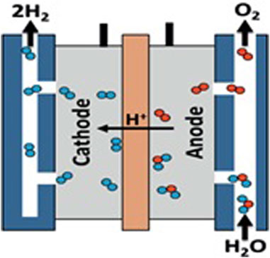
FIGURE 1. Simple electrolyzer model.

After turning on the power supply and forming the anode and cathode, electrolysis can commence. The hydrogen proton has a +1 charge and is attracted to the cathode, as given in Eq. 1:

$2H^{+}\left(l\right)+2e^{-}\to H_2\left(g\right)(1)$

Since oxygen ions have a negative charge of −2, they are attracted to the anode and undergo oxidation to release electrons.

$2H_{2}O\left(l\right)\to O_2\left(g\right)+4H^{+}\left(g\right)+4e^{-}(2)$

Solid oxide electrolysis (SOE), polymer electrolyte membrane electrolysis (PEM), and alkaline water electrolysis (AWE) are all ways to do electrolysis. The main difference between each method of electrolysis is the type of electrolyte they use. At present, electrolysis of water to produce hydrogen is very expensive, hence just 4% of the world’s industrial hydrogen comes from this source (Kumar and Himabindu, 2019). However, by 2030 this share is anticipated to grow as there will be rising interest in renewable power and falling costs for hydrogen-production equipment. The most popular types of electrolyzers are broken down and compared in Table 1, which provides a summary of the most important specifications and operation principles for them (Kumar and Himabindu, 2019), (Omran et al., 2021).

TABLE 1

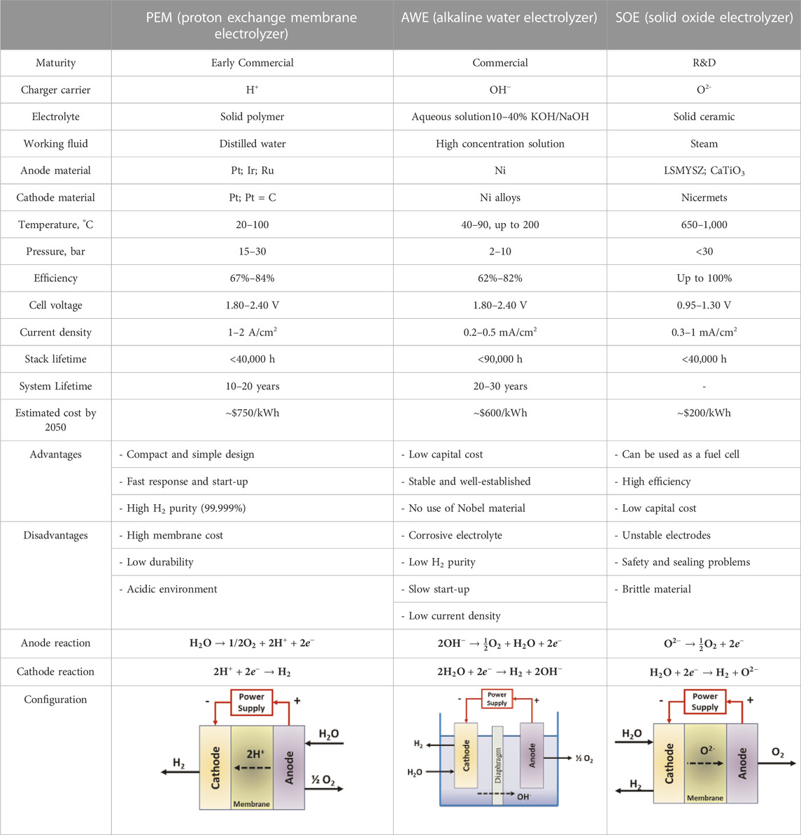
TABLE 1. Specifications and operation principles for different types of water electrolyzer.

2.1 Mathematical model for the proposed system components

To achieve the main goal of the paper, A proposed electrolysis system, which involves separating water into hydrogen and oxygen molecules, can be powered by solar energy in a system that is called a solar-powered water electrolysis system. This can be accomplished by employing photovoltaic, also known as PV, cells to create electricity from sunshine. This electricity can then be utilized to operate the electrolysis cell. As indicated in Figure 2, the proposed system consists of four major parts. In the power generation module, PV Solar System will be used to generate electricity. The second module is the water electrolyzer which is responsible for the separation of water into hydrogen and oxygen. A storage tank is required for storing the hydrogen output from the electrolyzer after compression using the compressor. Power conditioner units (DC-DC controllers) are responsible for regulating the required DC power for the electrolyzer.

FIGURE 2

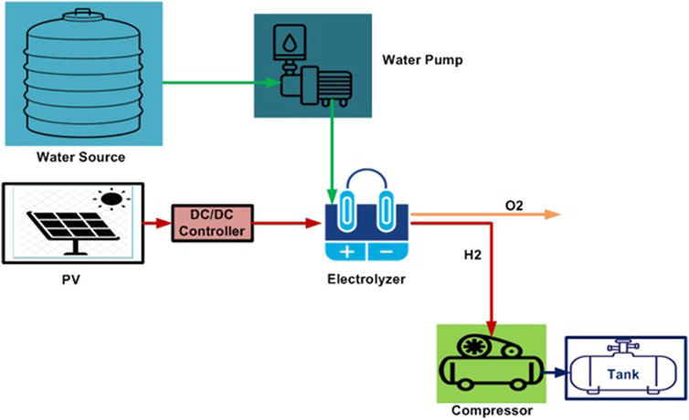
FIGURE 2. Schematic diagram for the proposed green hydrogen production system.

The mathematical model for the different components of the proposed production system is illustrated below:

2.1.1 Photovoltaic

The performance of the PV array can be simulated by first deriving the PV model, which reflects the maximum amount of power that can be output at any given temperature. The model that is being utilized is capable of predicting the output power of a PV panel under a variety of different temperature and radiation conditions. The following equations can be used to derive the mathematical model that was proposed for a photovoltaic panel (Yazdanpanah, 2014):

$P_{PV}=V.I\left(V\right)(3)$

$I\left(V\right)=\frac{I_x}{1-e^{\left(\frac{1}{b}\right)}}.\left[1-e^A\right](4)$

$A=\left(\frac{V}{b.V_x}-\frac{1}{b}\right)(5)$

$V_x=s.\frac{E_i}{E_{iN}}.TCV.\left(T-T_N\right)+s.V_{\mathit{max}}-B(6)$

$B=s.\left(V_{\mathit{max}}-V_{\mathit{min}}\right).e^C(7)$

$C=\left(\frac{E_i}{E_{iN}}.\mathit{ln}\left[\frac{V_{\mathit{max}}-V_{oc}}{V_{\mathit{max}}-V_{\mathit{min}}}\right]\right)(8)$

$I_x=p.\frac{E_i}{E_{iN}}.\left[I_{sc}+TCI.\left(T-T_N\right)\right](9)$

Where: P_PV is the output power of the PV panel (W), I(V) is the output current of the PV panel at a specific output voltage (A), V is the output voltage of the PV panel (V), b is the characteristic constant based on I-V curve its value ranges from 0.01 to 0.18., SRi is the solar radiation impinging the cell (W/m²), SRiN is the solar radiation at Standard Test Condition (STC) (=1000 W/m²), TN is the temperature at STC (= 25°C), Isc is the short circuit current at STC (A), Voc is the open circuit voltage at STC (V), Vmax is the open circuit voltage at 25 °C and 1200 W/m² (V), Vmin is the open circuit voltage at 25 °C and 1200 W/m² (V), T is the temperature of PV panel (°C), TCI is the temperature coefficient of Isc (A/°C), TCV is the temperature coefficient of Voc (V/°C), Ix is the short circuit current at any solar radiation and panel temperature (A), Vx is the open circuit voltage at any solar radiation and panel temperature (V), s is the number of PV panels in series, p is the number of PV panels in parallel. Table 2 shows the detailed PV module parameters.

TABLE 2

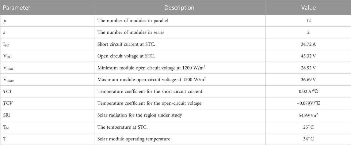
TABLE 2. Specifications and description principles for different parameters of PV module.

The following equation is used to calculate the annual energy of PV arrays at a specific site with a given solar radiation.

$E_{PV}=P\left({SR}_x\right).\left(SW\right).\left(365\right)(10)$

Where EPV refers to the amount of photovoltaic energy produced in a year. SW represents the total number of hours during which the Sun shines on the photovoltaic module, with an average hourly solar radiation. P(SRx) stands for the output power of the photovoltaic module at an average hourly solar radiation of SRx.

2.1.2 Electrolyzer

Proton exchange membrane, alkaline, and solid oxide electrolyzers are the three most common. The nature of the electrolyte determines how each type of electrolyzer operates. Hydrogen can be produced by either alkaline or PEM electrolyzers on-site and on-demand, with either kind producing hydrogen that is compressed without the need for a compressor and is also 99.999% clean, dry, and carbon-free. The following equations discuss the mathematical modeling for the alkaline type (Tijani et al., 2014).

$I=\frac{P_{EZ}}{V_{EZ}}(11)$

$V_{EZ}=V_{cell}\times n_c(12)$

$V_{cell}=V_{rev}+\left(\frac{r_{1+}{r}_2{T}_{EZ}}{A_{EZ}}\times I\right)+s\times \mathit{log}\left(\frac{t_1+\frac{t_2}{T_{EZ}}+\frac{t_3}{T_{EZ}^2}}{A_{EZ}}I+1\right)(13)$

${\eta }_F=\frac{{\left(\frac{I}{A_{EZ}}\right)}^2}{f_1+{\left(\frac{I}{A_{EZ}}\right)}^2}\times f_2(14)$

${\dot{n}}_{H2}=2{\dot{n}}_{O2}={\eta }_F\frac{I{n}_c}{zF}(15)$

Where PEZ represents the power of the electrolyzer. I and VEZ refer to the input current, measured in amperes, and the electrolyzer voltage, measured in volts, respectively. Vrev denotes the reversible cell voltage, while r represents the ohmic resistance. T is the overvoltage coefficient, s is the electrode overvoltage, TEZ is the electrolyzer operating temperature, AEZ is the electrode area, ηF is the Faraday efficiency, F is the Faraday constant, which is equal to 96,485 coulombs per mole, and $\dot{n}$ is the molar flow rate, measured in moles per second. The mathematical equation to calculate the amount of hydrogen in kg/day from daily solar energy data using a water electrolysis system is formulated as follows (Nasser et al., 2022). Table 3 shows the detailed electrolyzer model parameters.

$Q_{H2}=\frac{E*\eta *3600}{2*F}(16)$

TABLE 3

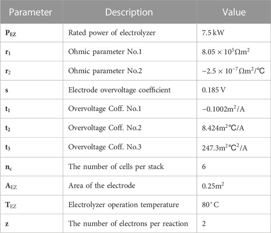
TABLE 3. Electrolyzer model parameters.

Where E is the forecasted solar energy per day in watts-hours, and $\eta$ is the efficiency of the PEM electrolyzer which is 77%.

2.1.3 DC-DC controller

The PV controller’s primary function is to regulate voltage. Shunt controllers, single-stage series controllers, diversion controllers, Pulse Width Modulation (PWM) controllers, and Maximum Power Point Tracking (MPPT) controllers are the five main varieties of PV controllers. In this section, the MPPT controller is applied to PV systems. This controller follows the array’s MPP throughout the day so that it can feed the most solar power into the system. To determine how many controllers (Ncon) a PV array will need, consider the following equation.

$P_{controller}=N_{PV}{\times V}_{OC}\times I_{SC}(17)$

Where, $N_{PV}$ is the total number of PV modules, and P_controller is the rated power of the controller for the PV system.

2.1.4 Compressor and storage tank

The compressor is used to compress the hydrogen output from the electrolyzer to store it in the tank. The mathematical model for the compressor is given below (Yavuz, 2020).

$P_{comp}=\frac{{\dot{n}}_{H2}\times \sum W_{stage}}{{\eta }_c}(18)$

$W_{stage}=\frac{n}{n-1}RT\left[1-{\left({rp\_}_{stage}\right)}^{\frac{n-1}{n}}\right](19)$

Where W_stage refers to the work performed by each compressor stage, measured in watts. rp_stage represents the pressure ratio per stage (rp__stage = 2.885). R is the universal gas constant, measured in joules per kelvin mol. T refers to the temperature of the hydrogen gas, measured in Kelvin. n is the polytropic index (n = 1.476), and ηc is the efficiency of the compressor (95%). Pcomp represents the total power consumed by the compressor, measured in watts. Given that the operating range of the system is below 200 bars, the pressure of the hydrogen gas tank is defined as follows:

$P_{tank}=\frac{{\dot{n}}_{H2}RT}{V_{tank}}(20)$

Where the P_tank and V_tank are the hydrogen tank pressure in Pascal and volume in m³.

2.2 Proposed hydrogen production forecasting algorithm

Forecasting hydrogen production from solar energy often entails assessing data on solar irradiance, temperature, and other parameters that impact the efficiency of solar panels. This is because solar panels are susceptible to being affected by a variety of environmental conditions. The following is a proposed framework for developing a hydrogen production forecasting algorithm:

1. Data collection: Collect historical data on solar irradiance, temperature, pressure, and humidity for the specific location where hydrogen production is planned.

2. Data preprocessing: Clean the data to remove any missing values or outliers that could skew the analysis.

3. Feature selection: Identify which features (solar irradiance, temperature) have the greatest impact on hydrogen production and select them into suitable inputs for the forecasting model.

4. Model selection: Choose an RNN machine learning algorithm that is appropriate for the Time-series data.

5. Model training: Train the model on the historical data to identify patterns and relationships between the features and hydrogen production.

6. Model evaluation: Evaluate the performance of the model using different metrics to determine the accuracy of the forecasts.

7. Deployment: Use the trained model to forecast future hydrogen production from solar energy based on incoming data on solar irradiance and temperature.

8. Regular updates: Regularly update the model as new data becomes available and retrain the model if necessary to ensure the forecasts remain accurate.

3 Materials and methods

This section describes the materials and procedures that were utilized in the course of carrying out the study. This section’s objective is to present readers with sufficient information to enable them to conduct their version of the research and evaluate the reliability of the findings.

3.1 Datasets

The datasets are meteorological data from the HI-SEAS weather station in Hawaii (Latitude: 19.5336° N Longitude: 155.5761° W) for 4 months (September through December 2016). We will forecast the level of solar radiation next season. For each dataset, the fields are Solar radiation: watts/m², Temperature: degrees Fahrenheit, Humidity: percent, Barometric pressure: Hg, Wind direction: degrees, Wind speed: miles per hour, and Sunrise/sunset: Hawaii time. The dataset is published on Kaggle as solar radiation prediction (Kaggle, 2017).

3.2 Data preprocessing

Data preprocessing is used to modify raw data so that it can be used in further analysis, modeling, and decision-making (Abdelhamid, et al., 2022). Errors, inconsistencies, and missing numbers are eliminated throughout the data-cleaning process using outlier analysis and data imputation (Alhussan, et al., 2022).

Data points that are extremely out of the norm are identified using outlier detection and eliminated from further analysis. The z-score method is used for outlier detection because it uses a distance metric to eliminate data points that are too far from the mean (Khafaga D. S. et al., 2022). We reconstruct the missing data points using median imputation to guarantee that the proposed algorithm acts effectively with full datasets (El-Kenawy et al., 2022a).

3.3 Recurrent neural network (RNN)

RNN is a specific kind of artificial neural network that was developed specifically to handle sequential input. RNNs have the ability to process sequences of inputs by retaining a “hidden state” that captures information about the previous inputs. This is in contrast to standard feedforward neural networks, which process inputs individually and do not have any recollection of past inputs. RNNs are able to do this because they do not process inputs independently (Shams, 2022). An RNN’s hidden state is changed at each time step by a combination of the most recent input and the state that was hidden before it, with the weights for this combination being learned beforehand. This enables the network to make predictions based on the history of the inputs while also capturing temporal dependencies in the data. RNN offers a wide variety of tools that can be used to solve problems with time series.

Because RNNs can interpret input sequences of varying lengths, they are particularly useful for a variety of applications, including natural language processing, speech recognition, and time series prediction, amongst others. This is one of the most significant advantages of RNNs. There are a few different varieties of RNNs, the most notable of which are the LSTM networks and the Gated Recurrent Unit (GRU) networks. Both of these types of RNNs have been demonstrated to be particularly successful in identifying long-term dependencies in sequential data.

The basic RNN with an input sequence x is a model that attempts to predict a state s_t at time t, taking into account the prior state s_t-1 by employing a differentiable function f. The prior state does not only include information from the previous time step; rather, it can be interpreted as a condensed version of all the states that have come before it. As shown in Figure 3, the weight parameters in RNN design, which are referred to as U, V, and W are shared across all layers (Aggarwal, 2018).

FIGURE 3

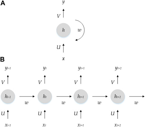
FIGURE 3. (A) RNN unit (B) Unfolded RNN unit showing the different time-steps state.

The next formulas are used to illustrate the corresponding relationships between them.

$s_t=f\left(s_{t-1}*W+x_t*U\right)(21)$

Where, s_t is the current hidden state at time step t, s_t-1 is the previous hidden state at time step t-1, x_t is the current input at time step t, W is the weight matrix that governs the influence of the previous hidden state, U is the weight matrix that governs the influence of the current input, f is the activation function that applies a non-linear transformation to the weighted sum of the inputs and previous hidden state, to produce the current hidden state.

$y_t=f\left(s_t*V\right)(22)$

Where y_t is the output at time step t, V is the weight matrix that governs the mapping between the hidden state and the output.

RNN models are trained to minimize a loss function, which is the amount of error in the predictions made in comparison to the values that occurred. During training, the RNN model is initially broken down into its constituent recurrent steps, as illustrated in Figure 3B. After that, the value of the gradient of the loss function concerning the output state at any instant. The estimated gradient is sent backward through the network at many time steps in order to complete the process. The formulas that follow represent, respectively, the recurring relationships and the accumulated gradients of parameters.

$\frac{\partial J}{\partial s_{t-1}}=\frac{\partial J}{\partial s_t}*W(23)$

Where: ∂J/∂s_t is the gradient of the loss function concerning the current hidden state at time step t, ∂J/∂s_t-1 is the gradient of the loss function for the previous hidden state at time step t-1 which is computed by back propagating the gradient through the current hidden state at time step t using the chain rule of differentiation.

$\frac{\partial J}{\partial U}={\displaystyle \sum _{t=0}^n}\frac{\partial J}{\partial s_t}*xt(24)$

Where: x_t is the current input at time step t, n is the length of the input vector, ∂J/∂U is the gradient of the loss function with respect to the weight matrix U that governs the influence of the current input on the current hidden state, which is computed by summing the product of the gradient with respect to the current hidden state and the current input over all time steps.

$\frac{\partial J}{\partial W}={\displaystyle \sum _{t=0}^n}\frac{\partial J}{\partial s_t}*s_{t-1}(25)$

Where: ∂J/∂W is the gradient of the loss function with respect to the weight matrix W that governs the influence of the previous hidden state on the current hidden state, which is computed by summing the product of the gradient with respect to the current hidden state and the previous hidden state over all time steps.

3.4 Particle Swarm Optimization (PSO)

In 1995, Kennedy and Eberhart were the ones who came up with the idea for the population-based optimization technique known as Particle Swarm Optimization, or PSO for short. The social behavior of birds flocking together and fish schooling, in which individuals coordinate their motions to pursue a shared goal, served as an inspiration for the development of the algorithm. PSO is a derivative-free optimization technique, which implies that it does not require any gradient information and may be used for solving non-linear and non-convex optimization problems. Because of this, PSO can be used to find optimal solutions to non-convex optimization problems.

The PSO algorithm creates a simulation of the behavior of a set of particles as they move across a multi-dimensional search space. Each particle in the simulation represents a potential solution to the optimization issue being solved by the algorithm. The algorithm keeps track of a population of particles, where each particle is distinguished from the others in the search space by its position and velocity over that space. In the context of the optimization problem, the position of a particle stands for a possible solution, while the velocity of a particle stands for the direction and speed at which it is moving. The method in which the particles move around in the search space is affected not only by their own experiences but also by the experiences of the particles around them (Mercangöz, 2021).

The PSO method kicks off by seeding a population of particles in the search space with a random distribution to get things started. The value of each particle’s goal function is determined so that the algorithm can determine how fit each particle is. The value of the objective function reflects the degree to which the potential solution embodied by the particle satisfies the requirements of the problem. The fitness of each particle is continually updated based on the value that it contributes to the objective function; a greater fitness value denotes a more promising candidate solution (Guo and Abdul, 2021).

After that, the PSO algorithm will make adjustments to the position Xi and velocity Vi of every particle that is currently present in the search space. Each particle’s velocity is updated depending on its current velocity, the distance it is from the best position it has found up to this point, as well as the distance it is from the best position found by its neighbors. The position of each particle is modified to reflect its most recent state by taking into account both its most recent velocity and its most recent position. This procedure is repeated by the algorithm for a predetermined number of times or until a stopping criterion is satisfied, whichever comes first (Khafaga, 2022b).

The velocity update equation for each particle i is given by:

$v_i^{t+1}=v_i^t+c_1{r}_1\left({Pbest}_i^t+x_i^t\right)+c_2{r}_2\left(g_{best}-x_i^t\right)(26)$

Where w is the inertia weight, c₁ and c₂ are the acceleration coefficients, r₁ and r₂ are random number between 0 and 1, ${Pbest}_i^t$ is the best position found by particle i, and $g_{best}$ is the best position found by the neighbors of particle i. The position update equation for each particle i is given by:

$x_i^{t+1}=x_i^t+v_i^{t+1}(27)$

The velocity vi of each particle is updated based on its current velocity, its distance from its best position found so far pi, and its distance from the best position found by its neighbors’ gj.

In order to attain desirable results with the PSO algorithm, it is necessary to tune its many adjustable parameters. The population size, the maximum velocity, the acceleration coefficients, and the topology of the neighborhood are all examples of these parameters. The maximum velocity restricts the greatest speed at which the particles can move, whereas the population size controls the number of particles that are contained inside the population. The acceleration coefficients govern the balance between the particle’s own experience and the experience of its neighbors, while the neighborhood topology dictates which particles are deemed to be neighbors of the particle in question.

3.5 Adaptive dynamic technique

After initializing the optimization algorithm, a fitness value is calculated for each solution in the population. The optimization method will then obtain the most relevant optimal agent in order to achieve the best possible fitness value (El-Kenawy et al., 2022b). As shown in Figure 4, the optimization algorithm begins the adaptive dynamic process by first dividing the population’s agents into two groups: exploring and exploiting. The primary goal of the exploiters is to advance toward the best solution, while the primary goal of the explorers is to probe the immediate vicinity of the leaders. The update that takes place between the different population groups and their agents is a dynamic process (El-Kenawy et al., 2022c). The optimization process starts with a population that is split evenly between the exploitation group and the exploration group (50/50) (Samee, et al., 2022). This is done so that the result will be a balanced relationship between the two groups.

FIGURE 4

FIGURE 4. Adaptive dynamic algorithm group balance between exploring and exploiting.

3.6 BER optimization algorithm

The Al-Biruni Earth Radius (BER) optimization algorithm is a metaheuristic algorithm that is based on the premise of recreating the process of measuring the radius of the Earth utilizing the method devised by the Persian scholar Abu Rayhan Al-Biruni in the 11th century. This approach was used to measure the radius of the Earth.

The technique begins by initially randomizing a collection of candidate solutions, which are comparable to the measurements of latitude and longitude that Al-Biruni took. After that, a fitness function is used to assess how well each candidate solution satisfies the optimization problem’s constraints. This function is designed to measure how well a solution satisfies the requirements. The possible solutions are then updated iteratively by the algorithm, imitating the procedure that Al-Biruni used to further hone the measurements (El-kenawy et al., 2023). During each iteration of the algorithm, a subset of the candidate solutions is chosen to serve as the “parents,” and a new set of candidate solutions, referred to as the “offspring,” is generated by employing genetic operators such as mutation and crossover. After that, the progeny is put through a fitness test, and the offspring with the best solutions are chosen to move on to the next-generation of candidate solutions. When a stopping requirement, such as a maximum number of iterations or a certain level of convergence, has been satisfied, the algorithm will come to an end.

The BER algorithm has been effectively utilized in the solution of a broad variety of optimization issues, such as function optimization, parameter tuning (Khafaga, 2022c), and feature selection. It is especially helpful for problems that involve a large number of variables and complex constraints, which are difficulties that other optimization techniques might have difficulty solving (Hamzah et al., 2022).

The proposed hybrid adaptive dynamic optimization based BER and PSO is discussed in Algorithm 1.

Algorithm 1. Proposed BER-PSO Algorithm

Set BERPSO population Xi (i = 1, 2, $\dots$, n), size n objective function Fn.

Collection configuration parameters

Function (Solution s) Fitness

Calculate fitness.

End Function While t < iter_Num

Calculate objective function F_n for each agent X_i

Set Z = best agent position

$r=h\frac{\mathit{cos}\left(x\right)}{1-\mathit{cos}\left(x\right)}$

$D=r_1\left(S\left(t\right)-1\right)$

$S\left(t+1\right)=S\left(t\right)+D\left(2r_2-1\right)$

In each group, Update the number of solutions.

If the best fitness did not improve,

Increase in the exploration group solutions number.

end if

for each solution in the exploration group

update r, D _and Z

The best solutions were elitism.

If Z < any of the best solutions mutate the solution by

$D=r_3\left(L\left(t\right)-S\left(t\right)\right)$

$S\left(t+1\right)=r^2\left(S\left(t\right)+D\right)$

$k$ decreases exponentially from 2 to 0 throughout iterations,

else

Search around current solution

$S^{\prime }\left(t+1\right)=r\left(S^{*}\left(t\right)+k\right)$

$k$ exponentially decreases from 2 to 0.

end if

end for

for each solution in the exploitation group

The best solutions

update r, D, _and Z

If Z < any of the best solutions

move towards the best solution.

$D=r_3\left(L\left(t\right)-S\left(t\right)\right)$

$S\left(t+1\right)=k{r}^2-h\frac{\cos x}{1-\cos x}$

else

search around the best solution

$v_i^{k+1}=v_i^k+c_1{r}_1\left({Pbest}_i^k+x_i^k\right)+c_2{r}_2\left(g_{best}-x_i^k\right)$

$x_i^{k+1}=x_i^k+v_i^{k+1}$

end if

end for

solutions

update fitness

end while

return best agent positionZ.

4 Simulation results

Green hydrogen production forecasting utilizing the provided AD-BER-PSO-RNN method is discussed, along with the experimental parameters and results. The simulation tests are broken up into two categories: ensemble forecasting and scenario comparison. The best accuracy of the proposed algorithm is tested against other algorithms in the literature by applying it to a variety of scenarios. In addition, the evaluated dataset undergoes a statistical examination of several tests to demonstrate the efficacy of the algorithm. Figure 5 depicts the actual values from the dataset as well as the values forecasted by the proposed AD-BER-PSO-RNN algorithm.

FIGURE 5

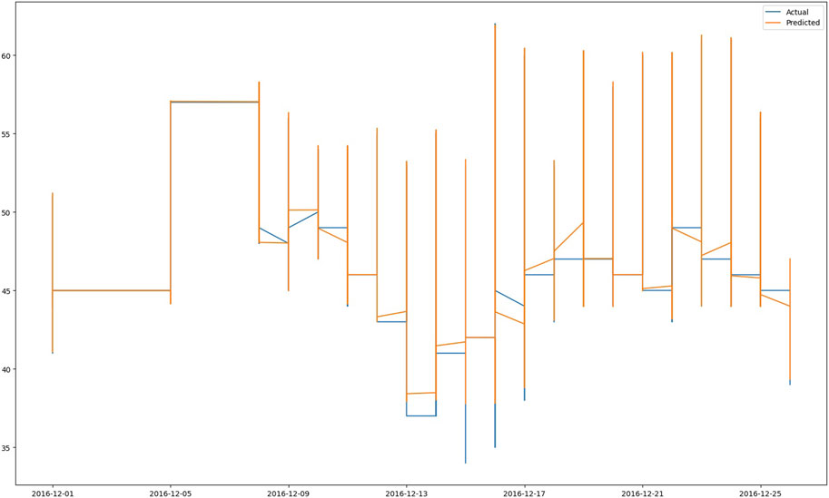
FIGURE 5. The actual (blue color) and forecasted (red color) values are based on the AD-BER-PSO-RNN algorithm.

When working with some datasets that do not make ideal candidates for feature selection, the residual values and plots can be of assistance (Saber, and Abotaleb, 2022). These datasets also contain the ones that are missing data. In order to achieve the optimal state, it is strongly suggested that the residual values be distributed uniformly over the horizontal axis. This will allow for the most accurate representation of the data. When calculating the value of the residual, the difference between the anticipated and actual values is used, and it is important to keep in mind that the sum of the residuals and their mean both equal zero. The plot of the residuals is shown in Figure 6, which may be found below. The patterns that are noticed in the plots of the residual data are used to select a non-linear model, a linear model, and finally, the best model is chosen from those two models. Figure 6 presents a plot of heteroscedasticity, which demonstrates the relationship between the two variables.

FIGURE 6

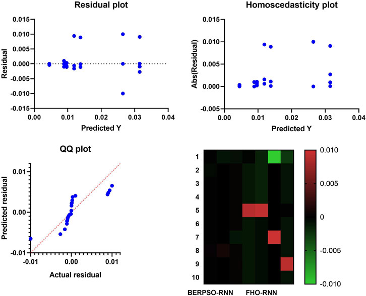
FIGURE 6. The Residual, heteroscedasticity, QQ plots, and heat map of the presented and compared algorithm for feature selection.

Homoscedasticity is a notion in statistics that indicates whether or not the error term is consistent across the values of the independent variables. Homoscedasticity can be defined as “whether or not the error term is consistent across the values of independent variables.” Figure 6 also includes a heat map, as well as quantile-quantile (QQ) plots, probability plots, and a representation of the probability of an event occurring. Because the point distributions in the QQ plot are so closely aligned with the preset line, it has come to our attention that the actual residuals and the forecasted residuals are related to one another in a way that can be described as a linear relationship. This provides further evidence that the AD-BER-PSO-RNN technique, which was demonstrated to be effective before, is indeed effective.

4.1 Ensemble forecasting

RNN ensemble-based models and an optimal ensemble model based on the AD-BER-PSO-RNN algorithm are used to construct this scenario. The training instances are used by some of the ensemble models. The Root Mean Squared Error (RMSE), as well as its relative counterpart, the Relative Root Mean Squared Error (RRMSE), the Mean Absolute Error (MAE), and the Mean Absolute Percentage Error (MAPE) which is comparable to MAE but is standardized using actual observations, and the correlation coefficient (r) are the assessment metrics that will be used in this scenario. The following equations discuss the mathematical formulas for the assessment metrics (Liu et al., 2019).

$RMSE=\sqrt{\frac{{\displaystyle \sum _{i=1}^n}{\left(z_{p,i}-z_i\right)}^2}{n}}(28)$

$RRMSE=\frac{RMSE}{{\displaystyle \sum _{i=1}^n}{z}_{p,i}}\times 100(29)$

$MAE=\frac{1}{n}{\displaystyle \sum _{i=1}^n}\left|z_{p,i}-z_i\right|(30)$

$MAPE=\frac{100}{n}{\displaystyle \sum _{i=1}^n}\frac{\left|z_{p,i}-z_i\right|}{z_{p,i}}(31)$

$r=\frac{{\displaystyle \sum _{i=1}^n}\left(x_i-\overline{x}\right)\left(y_i-\overline{y}\right)}{\sqrt{{\displaystyle \sum _{i=1}^n}{\left(x_i-\overline{x}\right)}^2{\left(y_i-\overline{y}\right)}^2}}(32)$

Where $n$ is the number of the total value, $z_{p,i}$ is the forecasted value, $z_i$ is the actual value, $x_i,y_i$ are the individual data points in the sample, and $\overline{x},\overline{y}$ are the sample means of the individual values. Table 4 shows the results for the different assessment metrics of the proposed AD-BER-PSO-RNN algorithm. The comparative descriptive statistics of the provided optimal ensemble model with those of other models are described and presented in Table 5.

TABLE 4

TABLE 4. Results of different assessment metrics of the proposed AD-BER-PSO-RNN algorithm.

TABLE 5

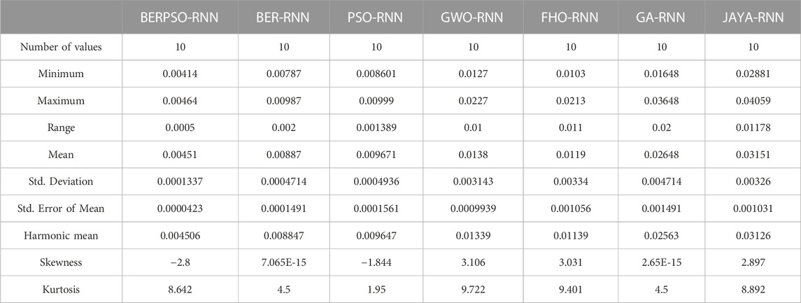
TABLE 5. Optimizing ensemble model’s descriptive statistics versus other models.

4.2 Stability analysis

The RMSE distribution is shown in Figure 7, and the histogram of RMSE is shown in Figure 8. These two figures are utilized to determine the stability of the suggested optimizing ensemble approach concerning the models that are compared.

FIGURE 7

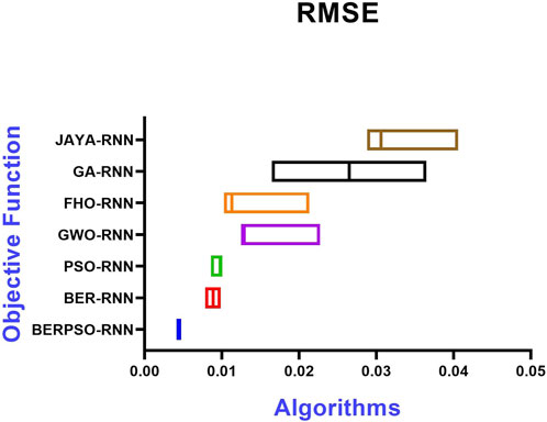
FIGURE 7. RMSE based on the objective function of the presented optimizing ensemble model and other models.

FIGURE 8

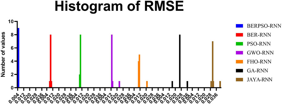
FIGURE 8. The Histogram of RMSE of the presented optimizing ensemble model and other models.

In this scenario, the analysis of variance (ANOVA) and the Wilcoxon rank-sum test (Wilcoxon test) is used to investigate the statistical discrepancies between the presented and compared models. Results from the ANOVA are shown in Table 6. Table 7 contains the results of a Wilcoxon rank-sum test used to determine whether or not the results of the different models differ significantly. In cases when the p-value is less than 0.05, significant superiority is shown.

TABLE 6

TABLE 6. ANOVA results of the base and ensemble models for solar energy forecasting.

TABLE 7

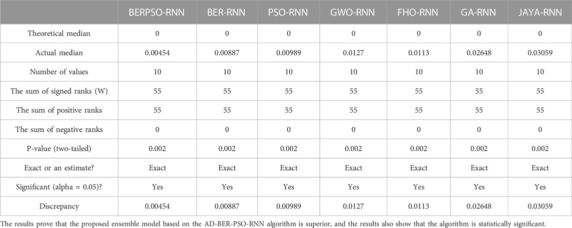
TABLE 7. Wilcoxon signed rank test results of the base and ensemble models for solar energy forecasting.

From an economical point of view, the proposed forecasting model plays a vital role in directing decision-making linked to investments in renewable energy, infrastructure design, and activities to minimize greenhouse gas emissions. Stakeholders can anticipate the future supply of hydrogen amount produced from solar energy using the proposed reliable forecasting model. So, investment decisions in renewable energy projects, such as solar and hydrogen production facilities, can benefit greatly from this data. Potential profits, project sustainability, and return on investment can all be evaluated. To further ensure that the produced hydrogen is put to good use, an accurate forecasting model can aid in optimizing the sizing and deployment of renewable energy systems. The proposed model can be used to inform the planning of infrastructure by revealing trends in hydrogen production and consumption. It helps decision-makers figure out how much infrastructure for storing, transporting, and distributing hydrogen will be needed. Infrastructure planners can make better decisions about the location, size, and configuration of hydrogen production, storage, and distribution networks if they have a clear picture of the total amount of hydrogen that will be available in the future. As a result, this improves the overall dependability of the hydrogen infrastructure while reducing costs and maximizing efficiency. Finally, solar-generated hydrogen offers a sustainable and environmentally friendly replacement for traditional fossil fuels. The presented model accurately predicts hydrogen production from solar energy, which helps in the development of plans and activities to lower GHG emissions. The anticipated data can be used by policymakers and environmental agencies to pinpoint potential integration points for solar hydrogen across sectors like transportation, industry, and power generation. Policymakers may stimulate the deployment of solar hydrogen technology and cut carbon emissions by connecting renewable energy goals with hydrogen demand estimates.

5 Conclusion

This study utilizes a dataset of solar energy as a case study, which was obtained from the Kaggle platform. The goal is to forecast daily solar power generation up to the following season. This information was gathered by Austin Energy, the local electric utility provider, for 4 months. The forecasting performance of the tested dataset is improved by a hybrid adaptive dynamic BER-PSO method that is proposed along with an optimization technique for a recurrent neural network. This allows for more accurate forecasting of the amount of hydrogen that is produced from a water electrolysis system. The proposed hybrid adaptive dynamic BER-PSO method chooses the best hyperparameters value of the RNN deep learning model for solar energy forecasting. The proposed algorithm is tested and compared to other algorithms, and it proved its superiority in terms of forecasting accuracy and computational efficiency through different metrics; RMSE, RRMSE, MAE, MAPE, and correlation coefficient. These results have significant ramifications for the creation of sustainable energy systems and policies, since accurate forecasting models may guide choices regarding investments in renewable energy, infrastructure design, and initiatives to reduce greenhouse gas emissions.

Data availability statement

The original contributions presented in the study are included in the article/Supplementary Material, further inquiries can be directed to the corresponding authors.

Author contributions

Conceptualization, E-SE-K; methodology, MS and E-SE-K; software, E-SE-K and AI; validation, OE, ME, and ME-S; formal analysis, LA and DK; investigation, E-SE-K and AI; writing—original draft, MS, E-SE-K, and ME; writing—review and editing, ME-S, AI, LA, and E-SE-K; visualization, ME, and DK; project administration, E-SE-K. All authors contributed to the article and approved the submitted version.

Funding

Princess Nourah bint Abdulrahman University Researchers Supporting Project number (PNURSP 2023R308), Princess Nourah bint Abdulrahman University, Riyadh, Saudi Arabia.

Conflict of interest

The authors declare that the research was conducted in the absence of any commercial or financial relationships that could be construed as a potential conflict of interest.

Publisher’s note

All claims expressed in this article are solely those of the authors and do not necessarily represent those of their affiliated organizations, or those of the publisher, the editors and the reviewers. Any product that may be evaluated in this article, or claim that may be made by its manufacturer, is not guaranteed or endorsed by the publisher.

References

Abdel-Nasser, M., and Mahmoud, K. (2019). Accurate photovoltaic power forecasting models using deep LSTM-RNN. Neural Comput. Appl. 31, 2727–2740. doi:10.1007/s00521-017-3225-z

CrossRef Full Text | Google Scholar

Abdelhamid, A. A., El-Kenawy, E. S. M., Khodadadi, N., Mirjalili, S., Khafaga, D. S., Alharbi, A. H., et al. (2022). Classification of monkeypox images based on transfer learning and the Al-Biruni Earth Radius Optimization algorithm. Mathematics 10 (19), 3614. doi:10.3390/math10193614

CrossRef Full Text | Google Scholar

Acar, C., and Dincer, I. (2019). Review and evaluation of hydrogen production options for better environment. J. Clean. Prod. 218, 835–849. doi:10.1016/j.jclepro.2019.02.046

CrossRef Full Text | Google Scholar

Aggarwal, C. C. (2018). “Recurrent neural networks,” in Neural networks and deep learning: A textbook (Heidelberg, Germany: Springer), 271–313. doi:10.1007/978-3-319-94463-0_7

CrossRef Full Text | Google Scholar

Alhussan, A. A., Khafaga, D. S., El-Kenawy, E. S. M., Ibrahim, A., Eid, M. M., and Abdelhamid, A. A. (2022). Pothole and plain road classification using adaptive mutation dipper throated optimization and transfer learning for self driving cars. IEEE Access 10, 84188–84211. doi:10.1109/ACCESS.2022.3196660

CrossRef Full Text | Google Scholar

Armijo, J., and Philibert, C. (2020). Flexible production of green hydrogen and ammonia from variable solar and wind energy: Case study of Chile and Argentina. Int. J. Hydrogen Energy 45 (3), 1541–1558. doi:10.1016/j.ijhydene.2019.11.028

CrossRef Full Text | Google Scholar

Aydin, M. I., and Dincer, I. (2022). An assessment study on various clean hydrogen production methods. Energy 245, 123090. doi:10.1016/j.energy.2021.123090

CrossRef Full Text | Google Scholar

El-kenawy, E. S. M., Abdelhamid, A. A., Ibrahim, A., Mirjalili, S., Khodadad, N., Al Duailij, M. A., et al. (2023). Al-Biruni Earth Radius (BER) metaheuristic search optimization algorithm. Comput. Syst. Sci. Eng. 45, 1917–1934. doi:10.32604/csse.2023.032497

CrossRef Full Text | Google Scholar

El-kenawy, E. S. M., Albalawi, F., Ward, S. A., Ghoneim, S. S., Eid, M. M., Abdelhamid, A. A., et al. (2022a). Feature selection and classification of transformer faults based on novel meta-heuristic algorithm. Mathematics 10 (17), 3144. doi:10.3390/math10173144

CrossRef Full Text | Google Scholar

El-Kenawy, E. S. M., Mirjalili, S., Abdelhamid, A. A., Ibrahim, A., Khodadadi, N., and Eid, M. M. (2022c). Meta-heuristic optimization and keystroke dynamics for authentication of smartphone users. Mathematics 10 (16), 2912. doi:10.3390/math10162912

CrossRef Full Text | Google Scholar

El-Kenawy, E. S. M., Zerouali, B., Bailek, N., Bouchouich, K., Hassan, M. A., Almorox, J., et al. (2022b). Improved weighted ensemble learning for predicting the daily reference evapotranspiration under the semi-arid climate conditions. Environ. Sci. Pollut. Res. 29 (54), 81279–81299. doi:10.1007/s11356-022-21410-8

CrossRef Full Text | Google Scholar

Elsaraiti, M., and Merabet, A. (2021). A comparative analysis of the arima and lstm predictive models and their effectiveness for predicting wind speed. Energies 14 (20), 6782. doi:10.3390/en14206782

CrossRef Full Text | Google Scholar

Erduman, A. (2020). A smart short-term solar power output prediction by artificial neural network. Electr. Eng. 102 (3), 1441–1449. doi:10.1007/s00202-020-00971-2

CrossRef Full Text | Google Scholar

Guo, L., and Abdul, N. M. M. (2021). Design and evaluation of fuzzy adaptive particle swarm optimization based maximum power point tracking on photovoltaic system under partial shading conditions. Front. Energy Res. 9, 712175. doi:10.3389/fenrg.2021.712175

CrossRef Full Text | Google Scholar

Hamzah, A. A., Nima, K., and Sunil, K. (2022). Improving the regression of communities and crime using ensemble of machine learning models. J. J. Artif. Intell. Metaheuristics 1 (1), 27–34. doi:10.54216/JAIM.010103

CrossRef Full Text | Google Scholar

Han, S., Qiao, Y. H., Yan, J., Liu, Y. Q., Li, L., and Wang, Z. (2019). Mid-to-long term wind and photovoltaic power generation prediction based on copula function and long short term memory network. Appl. energy 239, 181–191. doi:10.1016/j.apenergy.2019.01.193

CrossRef Full Text | Google Scholar

Intergovernmental Panel on Climate Change (2018). Global warming of 1.5° C: An IPCC special report on the impacts of global warming of 1.5° C above pre-industrial levels and related global greenhouse gas emission pathways, in the context of strengthening the global response to the threat of climate change, sustainable development, and efforts to eradicate poverty. Geneva, Switzerland: Intergovernmental Panel on Climate Change.

Google Scholar

International Energy Agency (2022). Global hydrogen review. Available online https://iea.blob.core.windows.net/assets/c5bc75b1-9e4d-460d-9056-6e8e626a11c4/GlobalHydrogenReview2022.pdf (Accessed June 6, 2023).

Google Scholar

Jawaid, F., and NazirJunejo, K. (2017). “Predicting daily mean solar power using machine learning regression techniques,” in 2016 Sixth International Conference on Innovative Computing Technology (INTECH), Dublin, Ireland, August, 2016 (IEEE) 355–360. doi:10.1109/INTECH.2016.7845051

CrossRef Full Text | Google Scholar

Kaggle (2017). Solar radiation prediction. Available online: https://www.kaggle.com/datasets/dronio/SolarEnergy (Accessed June 6, 2023).

Google Scholar

Kalogirou, S. A. (2001). Artificial neural networks in renewable energy systems applications: A review. Renew. Sustain. energy Rev. 5 (4), 373–401. doi:10.1016/S1364-0321(01)00006-5

CrossRef Full Text | Google Scholar

Khafaga, D., Ali Alhussan, A., M. El-kenawy, E. S., Ibrahim, A., H. Abd Elkhalik, S., El-Mashad, S. Y., et al. (2022c). Improved prediction of metamaterial antenna bandwidth using adaptive optimization of LSTM. Comput. Mater. Continua 73 (1), 865–881. doi:10.32604/cmc.2022.028550

CrossRef Full Text | Google Scholar

Khafaga, D. (2022b). Meta-heuristics for feature selection and classification in diagnostic breast cancer. Comput. Mater. Continua 73 (1), 749–765. doi:10.32604/cmc.2022.029605

CrossRef Full Text | Google Scholar

Khafaga, D. S., Alhussan, A. A., El-Kenawy, E. S. M., Ibrahim, A., Eid, M. M., and Abdelhamid, A. A. (2022a). Solving optimization problems of metamaterial and double T-shape antennas using advanced meta-heuristics algorithms. IEEE Access 10, 74449–74471. doi:10.1109/ACCESS.2022.3190508

CrossRef Full Text | Google Scholar

Khandakar, A., Eh Chowdhury, M., Khoda Kazi, M., Benhmed, K., Touati, F., Al-Hitmi, M., et al. (2019). Machine learning based photovoltaics (PV) power prediction using different environmental parameters of Qatar. Energies 12 (14), 2782. doi:10.3390/en12142782

CrossRef Full Text | Google Scholar

Kumar, S. S., and Himabindu, V. (2019). Hydrogen production by PEM water electrolysis–A review. Mater. Sci. Energy Technol. 2 (3), 442–454. doi:10.1016/j.mset.2019.03.002

CrossRef Full Text | Google Scholar

Liu, Q., Li, Z., Ji, Y., Martinez, L., Zia, U. H., Javaid, A., et al. (2019). Forecasting the seasonality and trend of pulmonary tuberculosis in Jiangsu Province of China using advanced statistical time-series analyses. Infect. drug Resist. 12, 2311–2322. doi:10.2147/IDR.S207809

PubMed Abstract | CrossRef Full Text | Google Scholar

Massaoudi, M., Chihi, I., Sidhom, L., Trabelsi, M., Refaat, S. S., and Oueslati, F. S. (2021). Enhanced random forest model for robust short-term photovoltaic power forecasting using weather measurements. Energies 14 (13), 3992. doi:10.3390/en14133992

CrossRef Full Text | Google Scholar

Mellit, A., and Pavan, A. M. (2010). A 24-h forecast of solar irradiance using artificial neural network: Application for performance prediction of a grid-connected PV plant at Trieste, Italy. Sol. energy 84 (5), 807–821. doi:10.1016/j.solener.2010.02.006

CrossRef Full Text | Google Scholar

Meng, M., and Song, C. (2020). Daily photovoltaic power generation forecasting model based on random forest algorithm for north China in winter. Sustainability 12 (6), 2247. doi:10.3390/su12062247

CrossRef Full Text | Google Scholar

Mercangöz, B. A. (2021). Applying particle Swarm optimization. Heidelberg, Germany: Springer International Publishing.

Google Scholar

Mohammed, I. J., Al-Nuaimi, B. T., and Baker, T. I. (2022). Weather forecasting over Iraq using machine learning. J. J. Artif. Intell. Metaheuristics 2 (2), 39–45. doi:10.54216/JAIM.020204

CrossRef Full Text | Google Scholar

Nasser, M., Megahed, T. F., Ookawara, S., and Hassan, H. (2022). Techno-economic assessment of clean hydrogen production and storage using hybrid renewable energy system of PV/Wind under different climatic conditions. Sustain. Energy Technol. Assessments 52, 102195. doi:10.1016/j.seta.2022.102195

CrossRef Full Text | Google Scholar

Omran, A., Lucchesi, A., Smith, D., Alaswad, A., Amiri, A., Wilberforce, T., et al. (2021). Mathematical model of a proton-exchange membrane (PEM) fuel cell. Int. J. Thermofluids 11, 100110. doi:10.1016/j.ijft.2021.100110

CrossRef Full Text | Google Scholar

Oubelaid, A., Shams, M. Y., and Abotaleb, M. (2022). Energy efficiency modeling using whale optimization algorithm and ensemble model. J. J. Artif. Intell. Metaheuristics 2 (1), 27–35. doi:10.54216/JAIM.020103

CrossRef Full Text | Google Scholar

Rana, M., and Rahman, A. (2020). Multiple steps ahead solar photovoltaic power forecasting based on univariate machine learning models and data re-sampling. Sustain. Energy, Grids Netw. 21, 100286. doi:10.1016/j.segan.2019.100286

CrossRef Full Text | Google Scholar

Saber, M., and Abotaleb, M. (2022). Arrhythmia modern classification techniques: A review. J. J. Artif. Intell. Metaheuristics 1 (2), 42–53. doi:10.54216/JAIM.010205

CrossRef Full Text | Google Scholar

Samee, N. A., El-Kenawy, E. S. M., Atteia, G., Jamjoom, M. M., Ibrahim, A., Abdelhamid, A. A., et al. (2022). Metaheuristic optimization through deep learning classification of COVID-19 in chest X-ray images. Comput. Mater. Continua, 4193–4210. doi:10.32604/cmc.2022.031147

CrossRef Full Text | Google Scholar

Shams, M. Y. (2022). Hybrid neural networks in generic biometric system: A survey. J. J. Artif. Intell. Metaheuristics 1 (1), 20–26. doi:10.54216/JAIM.010102

CrossRef Full Text | Google Scholar

Tijani, A. S., Yusup, N. A. B., and Rahim, A. A. (2014). Mathematical modelling and simulation analysis of advanced alkaline electrolyzer system for hydrogen production. Procedia Technol. 15, 798–806. doi:10.1016/j.protcy.2014.09.053

CrossRef Full Text | Google Scholar

United Nation (2015). Paris agreement. Available online: https://www.un.org/en/climatechange/paris-agreement (Accessed June 6, 2023).

Google Scholar

Wappler, M., Unguder, D., Lu, X., Ohlmeyer, H., Teschke, H., and Lueke, W. (2022). Building the green hydrogen market–Current state and outlook on green hydrogen demand and electrolyzer manufacturing. Int. J. Hydrogen Energy 47, 33551–33570. doi:10.1016/j.ijhydene.2022.07.253

CrossRef Full Text | Google Scholar

Xiaoyun, Q., Xiaoning, K., Chao, Z., Shuai, J., and Xiuda, M. (2016). “Short-term prediction of wind power based on deep long short-term memory,” in 2016 IEEE PES Asia-Pacific Power and Energy Engineering Conference (APPEEC), Xi'an, China, October, 2016 (IEEE) 1148–1152. doi:10.1109/APPEEC.2016.7779672

CrossRef Full Text | Google Scholar

Yavuz, H. (2020). Modelling and simulation of a heaving wave energy converter based PEM hydrogen generation and storage system. Int. J. Hydrogen Energy 45 (50), 26413–26425. doi:10.1016/j.ijhydene.2020.06.099

CrossRef Full Text | Google Scholar

Yazdanpanah, M. A. (2014). Modeling and sizing optimization of hybrid photovoltaic/wind power generation system. J. Industrial Eng. Int. 10, 49–14. doi:10.1007/s40092-014-0049-7

CrossRef Full Text | Google Scholar