 Yanwen Wang1
 Yanying Sun
 Yalong Li
- 1School of Mechanical and Electrical Engineering, China University of Mining and Technology-Beijing, Beijing, China
- 2Economic Research Institute of State Grid Zhejiang Electric Power Company, Hangzhou, China
Power systems faces significant uncertainty during operation owing to the increased integration of renewable energy into power grids and the expansion of the scale of power systems, these factors lead to higher load-loss risks; therefore, realization of a fast online load-loss risk assessment is crucial to ensuring the operational safety and reliability of power systems. This paper presents an online load-loss risk assessment method for power systems based on stacking ensemble learning. First, a traditional load-loss risk assessment method based on power flow analysis was constructed to generate risk samples. The label of the sample is load-loss risk assessment index and the features are multiple operational variables of the power system. And the recursive feature elimination using cross validation (RFECV) was adopted for feature selection. Second, four different machine learning models, including support vector regression (SVR), extremely randomized trees (ET), extreme gradient boosting (XGBoost) and elastic network (EN) were used to form a stacking ensemble learning model for sample training. Moreover, to further improve the model performance, the particle swarm optimization (PSO) algorithms was used for parameter optimization. Finally, based on this model, the online load-loss risk assessment of a power system was realized. The application of the proposed method on IEEE test systems demonstrated that the proposed method was more accurate than methods based on individual machine learning models, from which the stacking was designed, while still maintaining a significant advantage in terms of runtime compared to the traditional risk assessment method.
1 Introduction
With the increasing integration of renewable energy sources into power systems and growing load demands, the power system structure is becoming more complex. A power system is subject to a large variety of uncertainties during its operation, such as renewable energy output fluctuations, load fluctuations, and component failures, which lead to a rise in the risk of load shedding caused by generation–load imbalance or violation of safe operational limits, and these factors reduce the reliability and economy of the system operation.
Power system operational risk assessment is a comprehensive measure of the probability and severity of random disturbances that may occur in a power system within a given time scale (Li et al., 2015; Ansari and Chung, 2019; Ansari et al., 2020). This measure can help dispatchers ascertain the level of load-loss risk of a power system in a timely manner and formulate corresponding risk control strategies to ensure operational safety. This has become an indispensable task in the current-day power sector. The standard process of power system risk assessment, which is complex and time consuming, is as follows: first, probabilistic modeling of each part of the system, such as loads, wind farms, and units, is conducted. Then, using enumeration or the Monte Carlo method, a large number of possible states of the system are generated. This is followed by quantifying the severity of each possible state based on the power flow analysis. Finally, the risk index of the system, based on the probabilities of all the possible states and their severity values, is calculated (Wenyuan, 2014; Wang et al., 2019; Lin et al., 2023).
Using the results of risk assessment to support online scheduling that is minutes or hours ahead requires a fast and accurate calculation of risk indices. Over the past decades, many fast risk assessment methods have been proposed, and most of them have focused on improving the process of generating possible states of the system; this accelerates the convergence process of risk index calculation by generating possible states that contribute more to the risk index, thereby reducing the computational effort. Liu derived a fast sorting algorithm by a pre-process that arranges the system components in a descending order of their outrage rate, which can select the required number of system states in a descending probability order (Liu et al., 2008). Jia improved Liu’s method by arranging system components based on the severity coefficients determined by both their outrage rate and outage capacity and reduced the computational effort by defining the replaceable neighboring states of a state (Jia et al., 2013). Zhao, Yan, and Geng introduced importance sampling, and Shu and Taghavi introduced the Latin hypercube sampling method to improve the computational speed of risk indexes (Shu et al., 2014; Yan et al., 2017; Geng et al., 2019; Zhao et al., 2019; Taghavi et al., 2022). As quantifying the severity of possible states through power flow analysis is the most time-consuming process in risk assessment, efforts have been made to improve the computational speed by improving the power flow model used for severity quantification. Hou proposed a fast optimal load shedding method based on the shadow price theory (Hou et al., 2022). Zuo converted the optimal power flow model into a multi-parameter linear programming model to speed up the risk assessment (Zuo et al., 2022).
The abovementioned studies have effectively improved the risk assessment efficiency. However, with the rapid expansion of the scale of power systems owing to the growth of renewable energy integration capacity and load demands, the number of possible states to be analyzed in the online risk assessment of power systems has also increased dramatically; this increases the computational pressure further, requiring further exploration of new theories and techniques.
The development of artificial intelligence facilitated new solutions to online risk assessment of a power system. Based on the training of a large number of samples, machine learning methods can directly establish the mapping between the input and output features, thereby eliminating the complex intermediate process and reducing the computation time; this is highly suitable for the problem of online risk assessment; therefore, in recent years, there have been some research studies on machine learning-based risk assessment of power systems (Alimi et al., 2020; Gholami et al., 2020; Mehrzad et al., 2023; Prusty et al., 2023). Yun used the static voltage stability margin as a severity index of the possible state of a power system for voltage safety risk assessment and introduced a support vector machine (SVM) to achieve a rapid calculation of severity while optimizing the parameters of the SVM by the genetic algorithm (Yun et al., 2017). To improve the computational speed of the dynamic risk assessment of power systems, Jaiswal classified the contingencies into two categories, namely, security and insecurity, and trained a random forest (RF) with voltage magnitude and phase, current magnitude, real power, and reactive power as features and the contingency categories as labels (Jaiswal et al., 2019). Liu applied iterative random forests to calculate the severity of possible system states for dynamic security risk assessment of power systems (Liu et al., 2020). Jia established a mapping relation between N-k cascading contingencies and the severity index based on a random vector functional-link neural network (Jia et al., 2015). Li trained a multi-step adaptive LASSO regression model to compute the severity index for each possible state of the power system by considering both node voltage and power (Li et al., 2018). Jmii trained an artificial neural network to quickly determine whether a possible state of the power system is insecure (Jmii et al., 2019). Yang proposed a deep-learning method based on a stacked denoising auto-encoder network to achieve optimal power flow in a fast manner for risk assessment (Yang et al., 2019). Du transformed the computation of the severity index into a multi-classification problem and used convolutional neural networks to achieve fast classification of N-1 contingencies (Du et al., 2019). Li developed an extreme gradient boosting (XGBoost) regression model, and Zhu proposed an end-to-end machine learning model to quantify the relationship between uncertain parameters and risk indexes (Li et al., 2022; Zhu and Singh, 2023). Zhang used multiple extreme learning machines to form an ensemble learning model to quickly classify the risk level of the system state, and the results show that the classification accuracy of the integrated learning model is better than that of an individual learning model (Zhang et al., 2017).
The abovementioned studies have laid a good foundation for machine learning-based risk assessment methods for power systems; however, most of these studies have only used a single machine learning model; as there may be multiple mappings that can all achieve good performance in data training, the mappings learned using a single model may result in a poor generalization performance owing to stochasticity. Ensemble learning models can synthesize the advantages of multiple individual models to improve performance, but there are fewer studies using ensemble learning models for power system risk assessment. To further improve the performance of machine learning-based risk assessment methods, this study formed a stacking ensemble learning model with multiple differentiated machine learning models and used it to realize the online load-loss risk assessment of a power system. The main contributions of this study are as follows:
A traditional risk assessment method based on power flow analysis is first constructed to generate risk samples. The label of the sample is the value of the system load-loss risk assessment index, and the features are multiple operational variables of the power system. Then, support vector regression (SVR), extremely randomized trees (ET), and XGBoost were used as base models, while elastic network (EN) was used as a meta-model to form the stacking ensemble learning model to learn the relationship between stochastic variables and the risk assessment index; on the other hand, recursive feature elimination using cross-validation (RFECV) and particle swarm optimization (PSO) algorithms were used for feature selection and parameter optimization. Based on this model, the online load-loss risk assessment of a power system was realized. This proposed risk assessment method still maintained a significant advantage in runtime over traditional risk assessment methods, was more accurate than methods based on individual machine learning models, and displayed a high potential for online applications.
The rest of this paper is structured as follows: Section 2 details the process of generating training samples and the feature selection method. Section 3 explains the principle of stacking ensemble learning and the design of the proposed stacking ensemble learning model. Section 4 describes the overall process of the online load-loss risk assessment method. Section 5 provides a case study, and Section 6 concludes the paper.
2 Risk sample generation and feature selection
2.1 Risk sample generation
The first step in applying the stacking ensemble learning model to the load-loss risk assessment of a power system is to construct a risk sample set for model training. The task of the stacking ensemble learning model in this study is to replace the process of possible state generation and severity quantification of possible states in traditional risk assessment methods, which is a supervised learning task. Each sample is of the form “feature vector-label,” in which the label of the sample is the value of the system risk index. This study chose the expected demand not supplied (EDNS) as the risk assessment index, as it is one of the most commonly used indices in assessing load-loss risks for power systems (Cao et al., 2022). The specific calculation formula is given as follows:
where
The feature vector can be taken from various power system operation variables related to the risk index value, such as the forecasting renewable generation output of the power system, forecasting load of the power system, scheduled output and scheduled start-up status of conventional units, and failure rate of conventional units and lines.
To guarantee the performance of the trained model, the risk samples should cover, as much as possible, the operating conditions that may occur in practice. The specific process is as follows:
After determining the domains of the power system operation variables based on the historical operational data of the system, a feature vector was formed by uniformly sampling each operation variable in its domain; this vector was then used as the baseline operating condition of the power system for risk assessment, and the corresponding risk assessment index could be calculated based on a traditional risk assessment method. The aforestated process was repeated until the desired number of risk samples was obtained.
The specific process of calculating the risk indices, based on the traditional risk assessment method for each feature vector, is as follows:
First, a large number of possible states of the power system were generated. In this study, the uncertainties of renewable energy generation, load, and system failure were considered; therefore, the complete system state consisted of the renewable generation level, system load level, and system failure. Among them, as renewable generation is the sum of its forecasting output and forecasting error, this study used the typical seven-interval discretization of the zero-mean continuous normal-distributed function to describe the forecasting error; therefore, seven possible renewable generation levels were obtained. Similarly, seven possible levels of load and their probabilities could be obtained by discretizing the normal distribution into seven one-standard-deviation-wide intervals. As for the system failure, in this paper, we used the improved fast sorting algorithm proposed by Jia to generate N-k failures (Jia et al., 2013). Then, the optimal power flow model proposed by Wang was used to calculate the shedding load for each possible state (Wang et al., 2023). Finally, the EDNS of the power system was calculated based on the probability of the possible states and their shedding loads.
The flowchart for risk sample generation is presented in Figure 1.

FIGURE 1. Flowchart of risk sample generation.
2.2 Feature selection based on the RFECV algorithm
Feature dimensions can grow rapidly with the scaling-up of a power system, leading to a dimensionality catastrophe. In addition, the irrelevant and redundant features can also degrade the performance of machine learning models.
The RFE algorithm is a wrapper algorithm that requires a machine learning model to implement feature selection (Upadhyay et al., 2021). The algorithm starts with all the features, ranks them based on the importance scores after model training, and removes one or more features with the lowest importance scores; this process is repeated until the number of remaining features reaches a desired number. However, it is difficult to determine the optimal number of features with this algorithm; furthermore, it cannot take into account the interactions among the features, which may lead to a deterioration of the model performance after certain features are removed. To make up for the shortcomings of the RFE algorithm, this study adopted the RFECV algorithm for feature selection; it can automatically determine the optimal number of features by averaging the model performance based on cross-validation. We chose the RF model combined with the RFECV algorithm for feature selection. The process of power system risk feature selection based on the RFECV algorithm is as follows:
(1) The original risk samples are input.
(2) The RF model with the current features is trained based on cross-validation, and the importance score of each feature and the performance evaluation index of the RF model are calculated. The RF model can measure the feature importance according to the Gini index or the error of the out-of-bag samples; the latter was chosen in this study (Jaiswal et al., 2019). The R-squared error (R2) was chosen to evaluate the model performance, the value of R2 was in the range (0, 1), and the model performed better when R2 tended to 1 (Alimi et al., 2020).
(3) The features are ranked in descending order according to their importance scores, and the last-ranked feature is removed from the current features.
(4) It is checked whether the number of features is equal to 0; if yes, then it means that sorting of all the features is complete; we return to (5); otherwise, we return to (2).
(5) The features corresponding to the RF model with the highest performance evaluation index are selected as the optimal features, and these features are output.
The flowchart of risk feature selection of the power system based on the RFECV algorithm is presented in Figure 2.
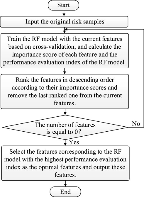
FIGURE 2. Flowchart of risk feature selection of the power system based on the RFECV algorithm.
3 Stacking ensemble learning model
3.1 Principles of stacking ensemble learning
The stacking ensemble learning model was first proposed by Worlpert in 1992; it consists of multiple base models and a meta-model, where multiple base models are trained with the same dataset, and then, the outputs of the base models are used as inputs to train the meta-model (Chatzimparmpas et al., 2021). Compared with a single machine learning model, the stacking model could reduce bias and decrease generalization errors.
The stacking ensemble learning model is usually trained based on cross-validation to reduce the risk of overfitting (Xie et al., 2021). If the original training set D contains m samples, then D is randomly divided into k subsets, with Di denoting the ith subset. For each base model, the subset Di is sequentially left out, and the remaining samples are used to train the base model; next, the ith trained base model is used to generate the output corresponding to the subset Di. According to the abovestated steps, the output of this base model for the entire original training dataset D can be generated after k trainings. The output of each base model is used as one-dimensional feature data for the training of the meta-model. If there are a total of J base models, J-dimensional feature data are generated in the end, which, together with the sample labels of the original training dataset, will form the training set
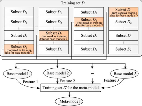
FIGURE 3. Principle of the stacking ensemble learning model.
3.2 Base model and meta-model
Although the stacking ensemble learning model has no strict limitation on the types of base and meta models, using multiple heterogeneous machine learning models as base models provides superior data mining capability from different spatial and structural perspectives. In addition, compared with the meta-model, the training samples of the base model have relatively higher feature dimensions; therefore, it is appropriate to adopt a base model with a more complex structure and a meta-model with a relatively simple structure.
In this study, three machine learning models were selected as base models: SVR, ET, and XGBoost.
It is assumed that the training sample set is
where
where
According to the Lagrange multiplier method, Eq. 3 can be transformed into its dual form, and finally, the SVR shown in Eq. 4 is obtained.
where
ET is an ensemble learning model consisting of multiple decision trees (Acosta et al., 2020). Unlike RT, ET uses the whole training set to train each individual decision tree, which helps to reduce the model bias. In addition, when performing decision tree node splitting, RF searches for the optimal cut point, while ET randomly draws the cut points and thresholds; this not only simplifies the node splitting procedure and reduces the computational load but also enhances the randomness of decision tree generation and reduces the model variance. The abovestated features of ET make it computationally efficient and difficult to overfit; therefore, we chose ET as one of the base models of the stacking ensemble learning model. It is constructed as follows: 1) the training set is input; 2) multiple replicas of the training set are generated by randomly sampling features; 3) for each replica, a decision tree with randomly split nodes is trained; and 4) the average of all the decision tree outputs is calculated as the output of ET.
XGBoost is an extension model for gradient boosting trees (Chen et al., 2018). It uses an objective function with a regularization penalty term to control the complexity of the model and adopts the feature subsampling technique, which not only effectively resists overfitting but also reduces the training time. Based on the abovestated advantages, this study selected XGBoost as one of the base models of the stacking ensemble model. The final output of the XGBoost consisting of K decision trees is given as follows:
where
In the tth iteration of the cumulative training, the tth decision tree can be obtained by minimizing the objective function, which is given as follows:
where
For the meta-model, this study chose the EN model (Chen et al., 2018), which is a combination of lasso and ridge regressions; thus, the model has the ability of the lasso regression model to drop the irrelevant features while maintaining the stability of the ridge regression model.
The objective function of the EN model is given as follows:
where
3.3 Parameter optimization based on the PSO algorithm
In this study, the PSO algorithm was introduced to optimize the parameters of the stacking model to further improve its performance.
The PSO algorithm transforms an optimization problem into a search process for the optimal position of a swarm of particles in the search space (Li and Jiang, 2011). If the stacking model has Q parameters to be optimized, a swarm of particles of size np and dimension Q is generated. The initial velocity and initial position of the particles are randomly generated in their feasible domains. The position of each particle represents a feasible solution to the stacking model parameters, and each dimension of the position corresponds to a parameter of the base model or meta-model. Each particle consecutively updates its position and velocity according to its own experience and the best experience of the swarm, to obtain the optimal solution after several iterations of updating the position of the particles. The optimal position of each particle and the swarm are determined based on the particle’s fitness value, and in this paper, R2 of the stacking model is chosen as the fitness function.
The flowchart for optimizing the parameters of the stacking ensemble learning model based on the PSO algorithm is shown in Figure 4.
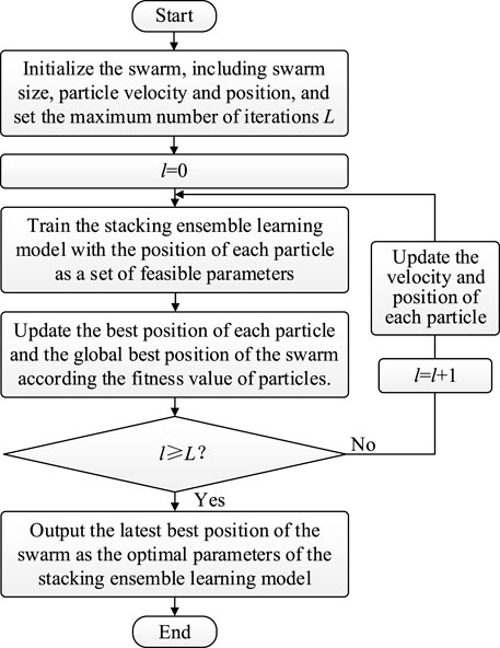
FIGURE 4. Flowchart for optimizing the parameters of the stacking ensemble learning model based on the PSO algorithm.
4 Online load-loss risk assessment of the power system based on stacking ensemble learning
Combining the contents in Section 2 and Section 3, the complete online load-loss risk assessment method of the power system, based on stacking ensemble learning, was obtained as described in (1–4) involved in offline modeling, and (5) realizes the fast online calculation of the risk index.
(1) Generation of risk samples based on historical power system operation data. Random sampling of the operation variables in their range, determined from historical data, was performed to form feature vectors; a traditional risk assessment method based on power flow analysis was used to calculate the corresponding risk index, i.e., EDNS, to form the power system risk samples.
(2) Feature selection based on the RFECV algorithm. Some of the features with low contributions to the risk index were removed by the RFECV algorithm to form the final training samples for the stacking ensemble learning model.
(3) Parameter optimization of the stacking ensemble learning model based on the PSO algorithm.
(4) Stacking ensemble learning model training. Using the optimal parameters determined by the PSO algorithm, three base models, namely, ET, XGBoost, and SVR, were trained based on cross-validation. The base models were used to generate training samples for the meta-model. The meta-model, i.e., the EN model, was then trained using the optimal parameters determined by the PSO algorithm. The trained base models and meta-model were combined to form the stacking model.
(5) Online calculation of the risk assessment index. Feature vectors for the moments to be assessed from power system online operation data were extracted and input into the trained stacking model. The corresponding risk assessment index could be calculated quickly, and subsequently, the schedulers could decide on the scheduling operations for these moments based on the risk level.
Figure 5 shows the online load-loss risk assessment method of the power system based on the stacking ensemble learning model.
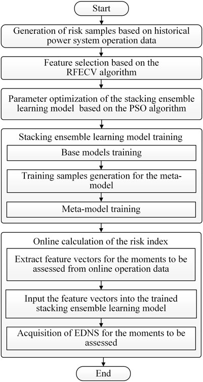
FIGURE 5. Online load-loss risk assessment method of the power system based on stacking ensemble learning.
5 Case study
5.1 Case introduction
The performance of the proposed online assessment method was demonstrated by applying it to the IEEE 24-bus system and IEEE 300-bus system. The IEEE 24-bus system contains 24 buses, 32 conventional units, and 38 lines, with a load peak of 2850 MW (Grigg et al., 1999). The topology of the IEEE 24-bus system is shown in Figure 6, and the installed capacity of the conventional units is presented in Table 1. The IEEE 300-bus system contains 300 buses, 69 conventional units, and 411 lines (University of Washington, 1993). As these two systems originally had no renewable energy sources, buses 18, 22, and 23 of the IEEE 24-bus system and buses 20, 60, 100, 150, 200, and 245 of the IEEE 300-bus system were selected for the wind power integration, with an installed capacity of 500 MW each.
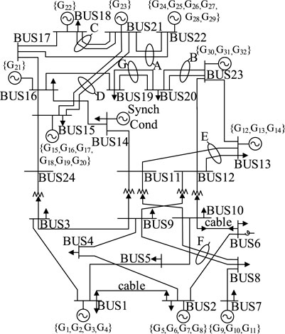
FIGURE 6. IEEE 24-bus system.
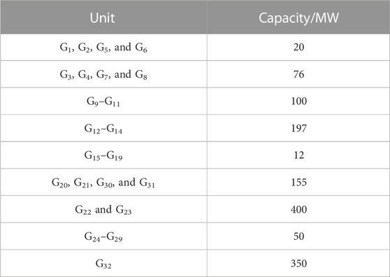
TABLE 1. Installed capacity of the conventional unit of the IEEE 24-bus system.
For the IEEE 24-bus system, the forecasting load of the system, forecasting wind power output of the system, failure rate of conventional units, scheduled start-up status of conventional units 20 and 22, and sum of the scheduled output of the conventional units were selected as features of the risk sample. The time scale for the risk assessment was taken as 1 h. The specific generation process of the risk samples was as follows: the forecasting load varied within [0.3, 1.2] based on the load peak, and the forecasting wind power output varied within [0, 1] based on its installed capacity. The failure rate of each conventional unit varied within [1 × 10⁻⁶, 1 × 10⁻⁴], and the rest of the equipment in the system was set to be 100% reliable, i.e., the failure rate was set to 0. Only the scheduled outages of conventional units 20 and 22 were considered; the probability of scheduled outage was set to 0.3, while the rest of the conventional units were scheduled to start up. The scheduled output of the conventional units was determined by the optimal power flow model based on the premise of generation–load balance under the randomly sampled forecasting wind power output and forecasting load. The installed capacity of each start-up unit was used as the weight of its scheduled output. Each time, after all the risk features were sampled, they were used as the baseline operating conditions of the system, and the EDNS was calculated according to the traditional risk assessment method described in Section 2.1. The standard deviation of the normal distribution for the wind power forecasting errors was set to 5% of the forecasting wind power output; the standard deviation of the normal distribution for the load forecasting errors was set to 1% of the forecasting load; and the number of N-k failures generated by the improved fast sorting method was set to 5,000. Using the abovementioned process, 20,000 risk samples with 37-dimensional features were obtained.
For the IEEE 300-bus system, the forecasting load of the system, forecasting wind power output of the system, failure rate of conventional units, scheduled start-up status of conventional units 11, 16, 28, 33, and 62, and sum of the scheduled output of the conventional units were selected as features of the risk sample. Only the scheduled outages of conventional units 11, 16, 28, 33, and 62 were considered when sampling the risk samples. The number of N-k failures generated by the improved fast sorting method was set to 10,000, and the rest of the settings were the same as those of the IEEE 24-bus system. A total of 50,000 risk samples with 77-dimensional features were obtained.
The symbols of the features for the IEEE 24-bus system and IEEE 300-bus system are presented in Table 2.

TABLE 2. Features of the risk sample.
The risk samples were divided into training and test sets in a ratio of 7:3 for the stacking model training and performance testing, respectively. The running environment is the WIN10 64-Bit system, Python platform.
Four indices, namely, the R2, mean square error (MSE), root mean square error (RMSE), and mean absolute error (MAE), were selected for the evaluation of the model performance. With the exception of R2, the smaller the indices, the smaller the difference between the values of the EDNS calculated by the model and their true values, and hence, the better the model performance.
5.2 Analysis of results
5.2.1 Feature selection results
The feature importance scores in the first iteration of the RFECV algorithm are presented in Figure 7.
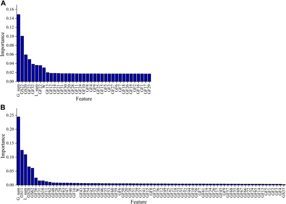
FIGURE 7. Feature importance scores of the features, (A) is feature importance scores of IEEE 24-bus system, (B) is feature importance scores of IEEE 300-bus system.
As can be seen in Figure 7, for the IEEE 24-bus system, the top 30% features included the sum of the scheduled output of conventional units (G_sum), the scheduled start-up status of units 20 and 22 (GS20 and GS22), the forecasting load of the system (L_sum), the forecasting wind power output of the system (W), and the failure rates of conventional units 22, 23, and 32 (GF22, GF23, and GF32). For the IEEE 300-bus system, the top 15% features included the sum of the scheduled output of conventional units (G_sum), the scheduled start-up status of units 11, 16, 28, and 62 (GS11, GS16, GS28, and GS62), the forecasting load of the system (L_sum), the forecasting wind power output of the system (W), and the failure rates of conventional units 31, 48 56, and 62 (GF31, GF48, GF56, and GF62).
For the IEEE 24-bus system, the importance scores of the failure rates of conventional units 22, 23, and 32 were significantly higher than those of the rest of the units, owing to the fact that the installed capacity of each unit was used as its weight in determining the scheduled output of the units in this case; thus, units with larger installed capacity would take on more loads, and their failures would cause a greater impact on the power balance of the system. Conventional units 22, 23, and 32 had higher installed capacity than the rest of the units; therefore, the load-loss risk was more sensitive to changes in the failure rates of these conventional units. For the same reason, the failure rates of conventional units 31, 48 56, and 62 of the IEEE 300 node system were ranked higher than the failure rates of the remaining conventional units of the system, and the scheduled start-up status of conventional unit 11, 16, 28, and 62 were ranked higher than the scheduled start-up status of conventional unit 33.
The optimal number of features selected by the RFECV algorithm for the IEEE 24-node system and the IEEE 300-bus node system was 18 and 29, respectively, and the R2 scores for different numbers of features are presented in Figure 8. The highest R2 score of 0.93 was achieved when 18 features were selected for the IEEE 24-bus system, and the highest R2 score of 0.91 was achieved when 29 features were selected for the IEEE 300-bus system, which removed some of the failure rates of conventional units with low installed capacities compared to the original features.
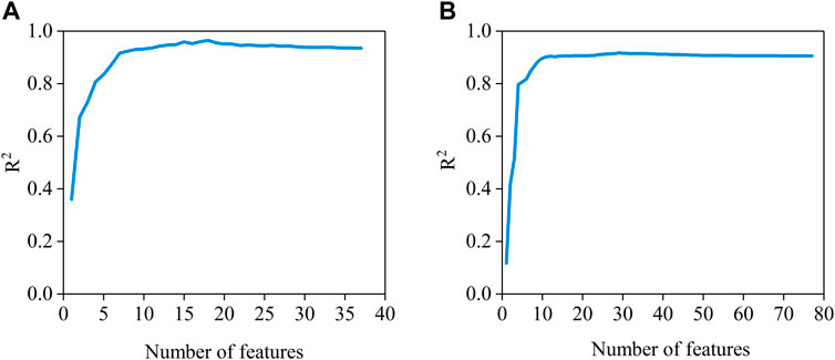
FIGURE 8. R2 scores for different numbers of features, (A) is R2 scores for IEEE 24-bus system, (B) is R2 scores for IEEE 300-bus system.
5.2.2 Parameter optimization results
The following parameters of the stacking ensemble learning model were optimized using the PSO algorithm: the number of decision trees (n_estimator) and the maximum number of features (max_features) for the ET; the penalty coefficient C and
The optimal parameters of the stacking ensemble learning model obtained by the PSO algorithm are presented in Table 3:
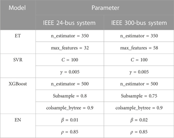
TABLE 3. Optimal parameters of the stacking ensemble learning model.
The stacking ensemble learning model was trained separately with optimal parameters and Python’s default parameters, and the scores of the performance evaluation indices of these two models on the test set are enumerated in Table 4.
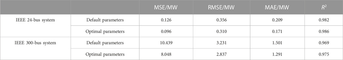
TABLE 4. Comparison of the performance evaluation indices of the stacking model with the optimal parameters and Python’s default parameters.
From Table 4, it can be seen that the MSE, RMSE, and MAE scores of the stacking ensemble learning model with optimal parameters were smaller than those of the stacking ensemble learning model with default parameters, and the R2 score of the stacking model with optimal parameters was larger than that of the stacking model with default parameters; this indicates that the model performance was improved after parameter optimization through the PSO algorithm.
5.2.3 Performance of the load-loss risk assessment method based on the stacking ensemble learning model
Figure 9 illustrates the EDNS calculated by the stacking model for 100 samples in the test set and the true value of the EDNS for the corresponding samples.
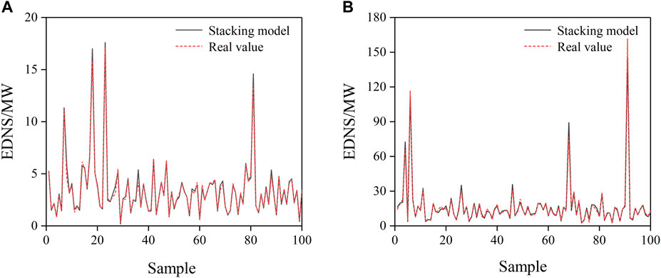
FIGURE 9. EDNS calculations for the test set of the load-loss risk assessment method based on the stacking ensemble learning model, (A) is EDNS calculations for IEEE 24-bus system, (B) is EDNS calculations for IEEE 300-bus system.
From Figure 9, it can be observed that the EDNS calculated by the stacking ensemble learning model was very close to its true value, indicating that the stacking ensemble learning model had only a small error.
To further illustrate the performance of the proposed method, this study used three base models of the proposed stacking ensemble learning model, i.e., ET, SVR, and XGBoost, for sample training separately. Table 5 shows the performance evaluation index scores of the risk assessment methods based on these different individual machine learning models. From Table 5, it can be seen that among the four methods, the one based on the stacking ensemble learning model had the lowest MSE, RMSE, and MAE scores and the highest R2 score.
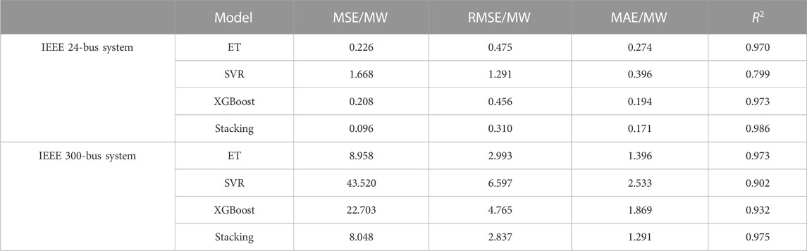
TABLE 5. Comparison of the performance indices of load-loss risk assessment methods based on different individual machine learning models and the proposed stacking model.
Three base models were used to form different stacking ensemble learning models for sample training, and the performance indices of the loss-of-load risk assessment methods based on different stacking ensemble learning models are shown in Table 6.
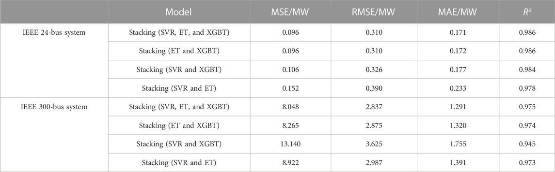
TABLE 6. Comparison of the performance indices of load-loss risk assessment methods based on different stacking ensemble learning models.
According to Table 5 and Table 6, removing any one of the three base models degrades the performance of the stacking ensemble learning model. For the IEEE 24-bus system, XGBT had the best performance among the three base models, and removing it had the greatest impact on the performance of the stacking integration model. Similarly, for the IEEE 300-bus system, removing the ET model with the best performance metric score from the base models had the greatest impact on the performance. This indicates that to ensure the performance of the stacking ensemble learning model, the model with its own good performance should be used as the base model.
The abovestated results indicate that compared to the risk assessment methods based on individual machine learning models, the one based on the stacking ensemble learning model combined the advantages of the multiple individual models and reduced the errors in calculating the risk assessment index.
EDNS calculations for the same number of risk samples were performed using the traditional load-loss risk assessment method described in Section 2.1, the proposed method, and the risk assessment method based on individual machine learning models, respectively. Table 7 displays the runtimes of these different risk assessment methods.
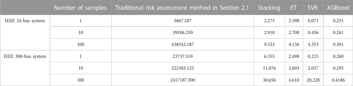
TABLE 7. Comparison of runtimes of load-loss risk assessment methods based on different machine learning models and the traditional load-loss risk assessment method (×10−2s).
As can be seen from Table 7, the stacking ensemble learning model required a longer time to compute the risk indices than its base models because it had a more complex structure. However, compared with the traditional load-loss risk assessment method, the proposed method still had a significant advantage in terms of runtime; thus, it ensured the timeliness of the assessment results, leaving more abundant time for risk control, and demonstrated excellent potential for online applications.
6 Conclusion
In this study, we developed a load-loss risk assessment method for power systems, using SVR, ET, XGBoost, and EN to construct a stacking ensemble learning model and the RFECV and PSO algorithms for feature selection and parameter optimization, respectively. The case results showed that compared with the risk assessment based on a single machine learning model, using the stacking ensemble learning model could combine the advantages of multiple machine learning models to achieve a more accurate calculation of the EDNS. Additionally, although the runtime of the load-loss risk assessment method based on the stacking ensemble learning model was longer than that based on a single machine learning model, it was still significantly shorter than that of the traditional risk assessment method; thus, the proposed method has a very good potential for online applications. Future research will focus on real-world applications of the proposed method and further improving the accuracy and runtime of the ensemble learning model for risk assessment of power systems.
Data availability statement
The raw data supporting the conclusion of this article will be made available by the authors, without undue reservation.
Author contributions
YW: conceptualization, project administration, supervision, and writing–review and editing. YS: methodology, supervision, and writing–original draft. YD: funding acquisition, project administration, and writing–review and editing. YL: methodology, writing–review and editing, and supervision. JC: software and writing–review and editing. XH: validation and writing–review and editing.
Funding
The authors declare financial support was received for the research, authorship, and/or publication of this article. This research was supported by the State Grid Zhejiang Electric Power Company Ltd. Science and Technology Project under grant no. 5211JY220004.
Conflict of interest
Author YD was employed by the Economic Research Institute of State Grid Zhejiang Electric Power Company.
The authors declare that this study received funding from State Grid Zhejiang Electric Power Company, LTD. The funder had the following involvement in the study: Writing–review & editing, Project administration.
The remaining authors declare that the research was conducted in the absence of any commercial or financial relationships that could be construed as a potential conflict of interest.
Publisher’s note
All claims expressed in this article are solely those of the authors and do not necessarily represent those of their affiliated organizations, or those of the publisher, the editors, and the reviewers. Any product that may be evaluated in this article, or claim that may be made by its manufacturer, is not guaranteed or endorsed by the publisher.
References
Acosta, M. R. C., Ahmed, S., Garcia, C. E., and Koo, I. (2020). Extremely randomized trees-based scheme for stealthy cyber-attack detection in smart grid networks. IEEE Access 8, 19921–19933. doi:10.1109/ACCESS.2020.2968934
Alimi, O. A., Ouahada, K., and Abu-Mahfouz, A. M. (2020). A review of machine learning approaches to power system security and stability. IEEE Access 8, 113512–113531. doi:10.1109/access.2020.3003568
Ansari, O. A., and Chung, C. Y. (2019). A hybrid framework for short-term risk assessment of wind-integrated composite power systems. IEEE Trans. Power Syst. 34 (3), 2334–2344. doi:10.1109/TPWRS.2018.2881250
Ansari, O. A., Gong, Y., Liu, W., and Chung, C. Y. (2020). Data-driven operation risk assessment of wind-integrated power systems via mixture models and importance sampling. J. Mod. Power Syst. Clean Energy 8 (3), 437–445. doi:10.35833/MPCE.2019.000163
Cao, M., Shao, C., Hu, B., Xie, K., Li, W., Peng, L., et al. (2022). Reliability assessment of integrated energy systems considering emergency dispatch based on dynamic optimal energy flow. IEEE Trans. Sustain. Energy 13 (1), 290–301. doi:10.1109/TSTE.2021.3109468
Chatzimparmpas, A., Martins, R. M., Kucher, K., and Kerren, A. (2021). StackGenVis: alignment of data, algorithms, and models for stacking ensemble learning using performance metrics. IEEE Trans. Vis. Comput. Graph. 27 (2), 1547–1557. doi:10.1109/TVCG.2020.3030352
Chen, P., Tao, S., Xiao, X., and Li, L. (2018). Uncertainty level of voltage in distribution network: an analysis model with elastic net and application in storage configuration. IEEE Trans. Smart Grid 9 (4), 2563–2573. doi:10.1109/TSG.2016.2614547
Chen, M., Liu, Q., Chen, S., Liu, Y., Zhang, C. H., and Liu, R. (2019). XGBoost-based algorithm interpretation and application on post-fault transient stability status prediction of power system. IEEE Access 7, 13149–13158. doi:10.1109/ACCESS.2019.2893448
Du, Y., Li, F., and Huang, C. (2019). “Applying deep convolutional neural network for fast security assessment with N-1 contingency,” in Proceeding of the 2019 IEEE Power & Energy Society General Meeting (PESGM), Atlanta, GA, USA, August 2019 (IEEE), 1–5.
Geng, L., Zhao, Y., and Li, W. (2019). Enhanced cross entropy method for composite power system reliability evaluation. IEEE Trans. Power Syst. 34 (4), 3129–3139. doi:10.1109/TPWRS.2019.2897384
Gholami, M., Sanjari, M. J., Safari, M., Akbari, M., and Kamali, M. R. (2020). Static security assessment of power systems: A review. Int. Trans. Electr. Energy Syst. 30 (9). doi:10.1002/2050-7038.12432
Grigg, C., Wong, P., Albrecht, P., Allan, R., Bhavaraju, M., Billinton, R., et al. (1999). The IEEE reliability test system-1996. A report prepared by the reliability test system task force of the application of probability methods subcommittee. IEEE Trans. Power Syst. 14 (3), 1010–1020. doi:10.1109/59.780914
Hou, K., Tang, P., Liu, Z., Jia, H., Yuan, K., Sun, C., et al. (2022). A fast optimal load shedding method for power system reliability assessment based on shadow price theory. Energy Rep. 8, 352–360. doi:10.1016/j.egyr.2021.11.104
Jaiswal, P. K., Das, S., and Panigrahi, B. K. (2019). “PMU based data driven approach for online dynamic security assessment in power systems,” in Proceeding of the 2019 20th International Conference on Intelligent System Application to Power Systems (ISAP), New Delhi, India, December 2019 (IEEE), 1–7.
Jia, Y., Wang, P., Han, X., Tian, J., and Singh, C. (2013). A fast contingency screening technique for generation system reliability evaluation. IEEE Trans. Power Syst. 28 (4), 4127–4133. doi:10.1109/TPWRS.2013.2263534
Jia, Y., Meng, K., and Xu, Z. (2015). N-K induced cascading contingency screening. IEEE Trans. Power Syst. 30 (5), 2824–2825. doi:10.1109/tpwrs.2014.2361723
Jmii, H., Meddeb, A., Abbes, M., and Chebbi, S. (2019). “An intelligent combination method for static security assessment,” in Proceeding of the 2019 International Conference on Advanced Systems and Emergent Technologies (IC_ASET), Hammamet, Tunisia, March 2019 (IEEE), 290–294.
Li, X., and Jiang, C. (2011). Short-term operation model and risk management for wind power penetrated system in electricity market. IEEE Trans. Power Syst. 26 (2), 932–939. doi:10.1109/TPWRS.2010.2070882
Li, X., Zhang, X., Wu, L., Lu, P., and Zhang, S. (2015). Transmission line overload risk assessment for power systems with wind and load-power generation correlation. IEEE Trans. Smart Grid 6 (3), 1233–1242. doi:10.1109/TSG.2014.2387281
Li, Y., Li, Y., and Sun, Y. (2018). Online static security assessment of power systems based on lasso algorithm. Appl. Sci. 8 (9), 1442. doi:10.3390/app8091442
Li, S., Ding, T., Mu, C., Huang, C., and Shahidehpour, M. (2022). A machine learning-based reliability evaluation model for integrated power-gas systems. IEEE Trans. Power Syst. 37 (4), 2527–2537. doi:10.1109/tpwrs.2021.3125531
Li, P., Wu, W., Wang, X., and Xu, B. (2023). A data-driven linear optimal power flow model for distribution networks. IEEE Trans. Power Syst. 38 (1), 956–959. doi:10.1109/TPWRS.2022.3216161
Lin, C., Bie, Z., and Chen, C. (2023). Operational probabilistic power flow analysis for hybrid AC-DC interconnected power systems with high penetration of offshore wind energy. IEEE Trans. Power Syst. 38 (4), 1–13. doi:10.1109/TPWRS.2022.3204707
Liu, H., Sun, Y., Wang, P., Cheng, L., and Goel, L. (2008). A novel state selection technique for power system reliability evaluation. Electr. Power Syst. Res. 78 (6), 1019–1027. doi:10.1016/j.epsr.2007.08.002
Liu, S., Liu, L., Fan, Y., Zhang, L., Huang, Y., Zhang, T., et al. (2020). An integrated scheme for online dynamic security assessment based on partial mutual information and iterated random forest. IEEE Trans. Smart Grid 11 (4), 3606–3619. doi:10.1109/tsg.2020.2991335
Mehrzad, A., Darmiani, M., Mousavi, Y., Shafie-Khah, M., and Aghamohammadi, M. (2023). A review on data-driven security assessment of power systems: trends and applications of artificial intelligence. IEEE Access 11, 78671–78685. doi:10.1109/ACCESS.2023.3299208
Prusty, B. R., Krishna, S. M., Bingi, K., and Gupta, N. (2023). “Risk-based reliability assessment of modern power systems using machine learning and probability theory,” in Proceeding of the 2023 International Conference on Artificial Intelligence and Applications (ICAIA) Alliance Technology Conference (ATCON-1), Bangalore, India, April 2023 (IEEE), 1–5.
Shu, Z., Jirutitijaroen, P., Silva, A. M. L. d., and Singh, C. (2014). Accelerated state evaluation and Latin hypercube sequential sampling for composite system reliability assessment. IEEE Trans. Power Syst. 29 (4), 1692–1700. doi:10.1109/TPWRS.2013.2295113
Taghavi, R., Samet, H., Seifi, A. R., and Ali, Z. M. (2022). Stochastic optimal power flow in hybrid power system using reduced-discrete point estimation method and Latin hypercube sampling. IEEE Can. J. Electr. Comput. Eng. 45 (1), 63–67. doi:10.1109/ICJECE.2021.3123091
University of Washington (1993). Power systems test case archive. http://labs.ece.uw.edu/pstca/.
Upadhyay, D., Manero, J., Zaman, M., and Sampalli, S. (2021). Intrusion detection in SCADA based power grids: recursive feature elimination model with majority vote ensemble algorithm. IEEE Trans. Netw. Sci. Eng. 8 (3), 2559–2574. doi:10.1109/TNSE.2021.3099371
Wang, L., Yuan, M., Zhang, F., Wang, X., Dai, L., and Zhao, F. (2019). Risk assessment of distribution networks integrating large-scale distributed photovoltaics. IEEE Access 7, 59653–59664. doi:10.1109/ACCESS.2019.2912804
Wang, Y., Sun, Y., Li, Y., Feng, C., and Chen, P. (2023). Risk assessment of power imbalance for power systems with wind power integration considering governor ramp rate of conventional units. Electr. Power Syst. Res. 217, 109111. doi:10.1016/j.epsr.2022.109111
Wenyuan, L. (2014). “Introduction,” in Risk assessment of power systems: Models, methods, and applications (IEEE), 1–14.
Xie, D., Zhou, Y., Wang, Z., Yang, Y., Yao, H., and Sun, H. (2021). “Total transfer capability evaluation of power systems based on stacking ensemble learning,” in Proceeding of the 2021 IEEE 4th International Electrical and Energy Conference (CIEEC), Wuhan, China, May 2021 (IEEE), 1–6.
Yan, C., Ding, T., Bie, Z., and Wang, X. (2017). A geometric programming to importance sampling for power system reliability evaluation. IEEE Trans. Power Syst. 32 (2), 1–1569. doi:10.1109/TPWRS.2016.2568751
Yang, Y., Yu, J., Yang, Z., Xiang, M., and Liu, R. (2019). “Fast calculation of probabilistic optimal power flow: A deep learning approach,” in Proceeding of the 2019 IEEE Power & Energy Society General Meeting (PESGM) (IEEE), 1–5.
Yun, Z., Zhou, Q., Feng, Y., Sun, D., Sun, J., and Yang, D. (2017). “On-line static voltage security risk assessment based on Markov chain model and SVM for wind integrated power system,” in Proceeding of the 2017 13th International Conference on Natural Computation, Fuzzy Systems and Knowledge Discovery (ICNC-FSKD), Guilin, China, July 2017 (IEEE), 2469–2473.
Zhang, Y., Xu, Y., Dong, Z. Y., Xu, Z., and Wong, K. P. (2017). Intelligent early warning of power system dynamic insecurity risk: toward optimal accuracy-earliness tradeoff. IEEE Trans. Industrial Inf. 13 (5), 2544–2554. doi:10.1109/TII.2017.2676879
Zhang, B., Wang, M., and Su, W. (2021). Reliability analysis of power systems integrated with high-penetration of power converters. IEEE Trans. Power Syst. 36 (3), 1998–2009. doi:10.1109/TPWRS.2020.3032579
Zhao, Y., Tang, Y., Li, W., and Yu, J. (2019). Composite power system reliability evaluation based on enhanced sequential cross-entropy Monte Carlo simulation. IEEE Trans. Power Syst. 34 (5), 3891–3901. doi:10.1109/TPWRS.2019.2909769
Zhu, Y., and Singh, C. (2023). Assessing bulk power system reliability by end-to-end line maintenance-aware learning. IEEE Access 11, 49639–49649. doi:10.1109/ACCESS.2023.3258680
Keywords: power system risk, online risk assessment, load-loss risk, stacking, ensemble learning
Citation: Wang Y, Sun Y, Dan Y, Li Y, Cao J and Han X (2023) Online load-loss risk assessment based on stacking ensemble learning for power systems. Front. Energy Res. 11:1281368. doi: 10.3389/fenrg.2023.1281368
Received: 22 August 2023; Accepted: 13 September 2023;
Published: 27 September 2023.
Edited by:
Zhengmao Li, Aalto University, FinlandReviewed by:
Chunyu Chen, China University of Mining and Technology, ChinaZiming Yan, Nanyang Technological University, Singapore
Copyright © 2023 Wang, Sun, Dan, Li, Cao and Han. This is an open-access article distributed under the terms of the Creative Commons Attribution License (CC BY). The use, distribution or reproduction in other forums is permitted, provided the original author(s) and the copyright owner(s) are credited and that the original publication in this journal is cited, in accordance with accepted academic practice. No use, distribution or reproduction is permitted which does not comply with these terms.
*Correspondence: Yalong Li, MjAxNzI2QGN1bXRiLmVkdS5jbg==