Power generation–network–load–energy storage co-planning under uncertainty

With the aggregation of renewable energy in the power system, the uncertainty caused by the renewable energy affects the planning and operation of power systems. Meanwhile, the existing planning models fail to consider renewable energy uncertainty methods, specifically concerning renewable energy confidence and future possible scenarios; thus, a confidence-based scenario cluster method is presented. A novel generator, network, load, and energy storage (GNLS) co-planning model is proposed in the paper. First, a confidence-based scenario cluster is built, which can reflect uncertainties by clustering and analyzing wind, solar, and load. Second, the proposed model focuses on load and energy storage co-planning, and in addition, relevant flexible indices are used to assess the model. Finally, the GNLS co-planning model is built as a bi-level stochastic model on continuous time scales. The model is solved using the Benders decomposition algorithm. The method in this paper is validated using an IEEE RTS 24-bus and a real test system in China to demonstrate the reduction in renewable energy curtailment and optimization of economic factors in power system planning.

1 Introduction

1.1 Background

The power industry facilitates carbon emission, and relevant new power systems ensure power security and high proportional renewable energy consumption. Traditional generators focus on power output controllable thermal power units, hydropower units, and generators with load regulation. Meanwhile, with large-scale renewable energy and distribution generators, the regulation capacity of generators is insufficient; therefore, the proportion of generators with high uncertainty increases, the tertiary industry and residents increase, and relevant network load characteristics deteriorate. Thus, the difference in the system peak and valley is enlarged, and the load rate decreases. Following this, power system uncertainty increases, and in this situation, flexible supply and demand balance is a challenge. Adequately regulating the flexibility of generator, network, load, and energy storage (GNLS) resources could ensure timely system response when the supply and demand vary (Saeed et al., 2021). Therefore, a secure system and reliable operational requirements are satisfied.

1.2 Literature review

GNLS co-planning is a crucial issue in new power systems; Yang et al. (2021) proposed generation–network–load planning containing various scenario requirements. In addition, high-proportional renewable energy integration in transmission grid expansion planning (Qiu et al., 2017; Zhuo et al., 2021) is illustrated from generation–network co-planning, network flexible planning, and transmission network planning perspectives. Coordinated with distribution network aspects (Zhuo et al., 2020), a transmission network planning framework is proposed based on high-proportional renewable energy integration. In generation-network co-planning (Yi et al., 2020) under an electricity market situation, the objective is maximum social welfare, generator-network co-planning model. With network expansion planning and coal-fired power units flexible retrofit (Wang et al., 2019; Wang et al., 2020a) co-planning model. In addition, for wind farms, the energy storage and transmission co-planning model proposed by Zhang et al. (2020) combines tie line control and unit commitment. For flexible planning targets, coordinated generation and energy storage expansion planning could ensure sufficient demand response. Existing studies consider flexible resources, flexible demand, and response balance in generation–network–energy storage planning models. For example, an investment decision and operational iteration model was proposed based on multi-timescale flexible planning (Rintamäki et al., 2024), and a co-planning model was constructed from four aspects, namely, from generation–generation co-planning, generation–energy storage co-planning, generation–network co-planning, and generation–load co-planning. Flexible assessment indices are embedded into the planning model, and flexible post-probability assessment indices (Abdin and Zo, 2018) are proposed after power system planning. In addition, Hamidpour et al. (2019) proposed a flexible index to increase flexibility by constructing a generator–network co-planning model with energy storage and demand side response.

Traditional power system planning primarily involves load prediction, generator planning, a transmission grid, and distribution grid (Liu et al., 2022a; Liu et al., 2022b). New power systems involve diverse structures, flexible resources, and vagueness between the generator and load; therefore, new power systems should consider multi-scenario, probabilistic, co-planning perspectives to satisfy higher security (Zhang et al., 2023; Zhang et al., 2021) requirements in future prospects. For scenario generation, Ziaee et al. (2018) correlated between wind and demand scenarios, specifically (Han et al., 2019), mid-to-long-term wind and photovoltaic power generation prediction are based on copula function. In summary, existing methodologies fail to consider the wind and solar output spatial–temporal correlation and seasonal difference; therefore, a seasonal multi-wind and solar output co-planning model is a gap that needs to be filled.

For uncertainty in planning, methods are primarily classified into two types: stochastic optimization approaches (Zhang et al., 2017) and robust optimization approaches (Zhang and Conejo, 2018; Liu et al., 2019). Stochastic planning (Li et al., 2022; Li et al., 2023a) converts an uncertainty optimization issue to a certain optimization issue at scenario sets. Different from stochastic planning, robust planning reflects uncertain factors as a bounded uncertain set and obtains decisions based on the worst scenarios. The above two approaches are adapted to cope with renewable energy uncertainty, load uncertainty, and fault uncertainty. Comparatively, stochastic planning is more mature than robust planning. Chance constraint (Chen et al., 2018; Li et al., 2023b) is involved in transmission grid expansion planning containing wind farms besides the joint consideration of the Monto Carlo simulation and analytic methods to acquire wind output probabilistic distribution. Chen et al. (2018) proposed a Wasserstein distance-based distributionally robust generation expansion planning that involves the uncertainty concerns and improves robust planning for conservative issues.

Rintamäki et al. (2024) and Wang et al. (2020b) proposed a short-time operational model of source-side planning that is adapted to large-scale renewable energy integration. While the above work focuses on the source side (Li et al., 2024) or transmission line co-planning, energy storage and load-side flexible resources have not been considered. However, the continuous-time renewable energy operational characteristics of diverse seasons are not adequately considered, and a multi-level self-adaptive robust planning model (Abdin et al., 2022) is presented, which utilizes bounded intervals to indicate the uncertainty of renewable energy. An adaptively stochastic method (Li et al., 2020; Li et al., 2021) is involved in two-layer planning.

1.3 Contributions and organization of the paper

The paper solves the issue of configuring flexible resources (Jin et al., 2021) for supporting the carbon target. This paper first constructed future reconstructed scenarios considering multi-seasonal scenarios according to flexible indices in multi-seasonal scenarios and analyzed flexible variation trends in multi-operational scenarios; then, when the objective function is the minimum of investment and operational cost, it constructs multi-flexible resources and a GNLS co-planning model, which is then solved by the Benders decomposition algorithm.

The paper fills the gap where renewable energy uncertainty is not considered both in historical and future scenarios; moreover, renewable energy operational characteristics of diverse seasons are not adequately considered on continuous time. In addition, case studies of existing research hardly contain a real test case; thus, the application limitations of the generator–network–load–energy storage model are obvious. Overall, the novelty of this paper is as follows:

1) A novel bi-level GNLS co-planning model is proposed on a continuous-time scale that incorporates uncertainty. The model involves energy storages, demand response, and renewable energy as decision variables in long time scale constraints, and it also imbeds short time scale operational simulation.

2) A spring, summer, autumn, and winter scenario cluster is first built. Wind, solar, and load are then clustered and analyzed to reflect uncertainties.

3) In addition to the IEEE case study, this paper innovatively contains a real 301 node large-scale test system that reflects the GNLS mode in industrial application.

2 Uncertainty model and flexible indices

The uncertainty model refers to a confidence-based wind and solar power output scenario cluster and reconstruction model. Flexible indices refer to flexible deficiency index, flexible deficiency time index, and flexible deficiency expectation index.

2.1 Uncertainty model

The uncertainty model considers the spatial–temporal correlation of wind and solar power output. Specifically, it considers wind output temporal self-correlation, solar output temporal self-correlation, and wind and solar spatial inter-correlation.

The confidence-based wind and solar power output scenario cluster and reconstruction process is depicted in Figure 1. First, a k-means cluster approach is applied to the wind, solar, and load scenario cluster. The cluster approach is used for historical scenarios. Data preprocessing is necessary; abnormal values are deleted, and the existing wind, solar, and load continuous time data are made up. Data integrity and accuracy is the pre-requisites for cluster analysis; the Gaussian filtering method is applied to delete abnormal data with a large difference, and the interpolation method is then used to make up missing data. Finally, the k-means cluster is used to obtain clustered wind, solar, and load data.

Figure 1

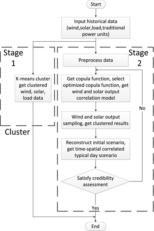
Figure 1. Confidence-based wind and solar power output scenario cluster and reconstruction process.

The second stage is wind and solar power output scenario reconstruction. First, historical scenario data are collected and processed. Then, the copula function is utilized to obtain the wind and solar output correlation model. Subsequently, joint probability distribution function is used at various time scales to sample, follow up, and cluster the sampled results, and obtain a typical-day scenario with wind and solar power output. Finally, wind and solar credibility is calculated after reconstruction, as in Eq. 1. If the calculation results cannot satisfy the credibility assessment, feedback is provided to the process to regulate parameters.

${\displaystyle \sum _{t\in T}}{R}_t\left\{P_{n,t}+{\displaystyle \sum _{g\in G}}{C}_g,d_t\right\}={\displaystyle \sum _{t\in T}}{R}_t\left\{C_c+{\displaystyle \sum _{g\in G}}{C}_g,d_t\right\},(1)$

where $R_t$ is the system reliability, $P_{n,t}$ is renewable energy at site n, $C_g$ is the capacity of traditional power units, $d_t$ is the load at time t, and $C_c$ is renewable energy credible capacity.

2.2 Flexible indices

(1) Flexible deficiency index (Eq. 2):

$P_{\gcd }\left(t\right)=\mathrm{Pr}\left\{{\displaystyle \sum _{i=1}^N}{P}_{rd}\left(i,t\right)<-\frac{\Delta L\left(t\right)}{\Delta t}\right\},(2)$

where $P_{rd}\left(i,t\right)$ is the ramp rate and $\frac{\Delta L\left(t\right)}{\Delta t}$ is the speed of net load variation. The index refers to assess renewable energy curtailment. The available down-ramp speed is less than load-drop speed, thus rendering renewable energy curtailment.

(2) Flexible deficiency times index (Eq. 3):

$P_{fdt}=\mathrm{Pr}\left\{F_{up}\left(t\right)<D_{up}\left(t\right),F_{down}\left(t\right)<D_{down}\left(t\right)\right\},(3)$

where the flexible deficiency time index simultaneously considers the total probability of upregulation deficiency and downregulation deficiency. F is the regulation capability and D is the demand.

(3) Flexible deficiency expectation index (Eq. 4):

$E_{fde}=\frac{{\sum }_{m=1}^M\left|\Delta L_{flex,m}\right|}{n\cdot P_{ren}},\Delta L_{flex,m}<0,(4)$

where $\Delta L_{flex,m}$ refers to the lack of flexibility, n is the flexible deficiency period, and $P_{ren}$ is the power system renewable energy installed capacity. The flexible deficiency expectation index accounts for the deficiency proportion where the flexible resource regulation capacity is less than the net load regulation requirement. Specifically, the system suffers load-shedding risk when up-flexible deficiency appears, and on the contrary, the system suffers renewable energy curtailment risk when down-flexible deficiency appears.

3 GNLS co-planning model

The objective of the model is mainly the minimization of the generator cost, line cost, and energy storage cost. In view of its complexity, the constraints of the continuous-time scale GNLS co-planning model are classified into long-term constraints and short-term constraints. Decision variables and state variables are set such as whether to adopt demand responses, the capacity and location of renewable energy, energy storages, thermal power units, hydraulic power units, and transmission lines.

3.1 Objective function

Objective function Eqs 5, 6 is the minimum investment cost $f_{inv}$, operational cost $f_{oper}$, and $f_{curt}$.

$\min f_{total}=f_{inv}+f_{oper}+f_{shed}+f_{cur}.(5)$

$\left\{\begin{array}{l}{f}_{inv}={\displaystyle \sum _{i=1}^{IN}}{x}_i{c}_i^I+{\displaystyle \sum _{k=1}^{KN}}{x}_k{c}_k^I+{\displaystyle \sum _{e=1}^{EN}}{x}_e{c}_e^I\\ f_{oper}={\displaystyle \sum _{s=1}^{N_S}}{\omega }_s\left({\displaystyle \sum _{i=1}^{IN}}\left(\Delta P_i{c}_i^M+p_i{c}_i^E\right)+{\displaystyle \sum _{b=1}^{N_B}}{p}_{ls,b,s}^{DR}{c}_b^{DR}\right)\\ f_{\text{she}d}={\displaystyle \sum _{s=1}^{N_S}}{\omega }_s{\displaystyle \sum _{b=1}^{N_B}}{p}_{\text{ls},b,s}{c}_y^L\\ f_{\text{cu}r}={\displaystyle \sum _{s=1}^{N_S}}{\omega }_s{\displaystyle \sum _{r=1}^{N_R}}{p}_{\text{rc},r,s}{c}_z^R\end{array}\right..(6)$

The scenario data on the four seasons given in Section 2 are applied in this section as wind and solar input data. $s$ is the scenario numeral order, ${\omega }_s$ is the scenario weight coefficient, and $N_s$ is the number of scenarios. Decision variables are conventional generators and renewable energy investment $x_i$, lines investment $x_k$, and energy storage investment $x_e$; IN is the number of conventional units and renewable energy, $c_i^I$ is the annual investment cost of generator units, $c_k^I$ is the annual investment cost of lines, $c_e^I$ is the energy storage annual investment cost, $c_i^E$ is the operational cost of various generators, $c_b^{DR}$ is the demand-side response cost, $c_y^L$ is the load-shedding penalty cost, and $c_z^R$ is the cost of renewable energy abandonment. IN, KN, and EN are the number of candidate power supply, lines, and energy storage, respectively. $N_B$ is the number of buses, and NR is the number of renewable energy fields.

3.2 Long-term constraints

1) Policy constraints:

$\begin{array}{l}\left\{\begin{array}{l}\Delta P_i\le P_i^{\max }\\ \Delta P_j\le P_j^{\max }\\ \Delta P_k\le P_k^{\max }\end{array}\right.\end{array},(7)$

where Eq. 7 is the various candidate units and flexible resources that are limited to the district resource endowment constraint. Here, ${P_i}^{\max }$ is the maximum limit of units, $P_j$ is the energy storage capacity, and the DR capacity is independent each year. $P_k$ is the demand response capacity.

$\frac{{\displaystyle \sum _{i=1}^n}{H}_i\Delta P_i}{{\displaystyle \sum _{i=1}^m}{H}_i\Delta P_i}\ge \alpha .(8)$

The above is the energy policy constraint, where ${\displaystyle \sum _{i=1}^n}{H}_i\Delta P_i$ and ${\displaystyle \sum _{i=1}^m}{H}_i\Delta P_i$ are non-fossil energy generation and total generation, respectively, and $\alpha$ is the non-fossil energy generation minimum proportion.

$\frac{\left(R_i^{\max }-R_i\right)}{R_i^{\max }}\le \chi .(9)$

The renewable energy sustainable development policy constraint Eq. 9 is diverse wind and solar curtailment upper limits in diverse districts. Here, $R_i$, $R_i^{\max }$, and $\chi$ are diverse renewable energy actual generation, maximum generation, and maximum wind and solar curtailment proportion, respectively.

2) Total reserve constraint (Eq. 10):

$\sum X_g{P}_{\psi ,\max }+\lambda \sum P_{r,\text{Install}}\ge \left(1+\alpha \right){\displaystyle \sum _{b\in \mathrm{\Xi }}}D,(10)$

where $\lambda$ is the renewable energy confidence capacity, $\alpha$ is a system reserve factor, $P_{r,\text{Install}}$ is the installed capacity of renewable energy r, and D is the peak load.

3.3 Short-term constraints

3) The node power balance constraint Eq. 11 is the balance between units, energy storage output, renewable energy output, and demand response power and load.

$\begin{array}{l}{\displaystyle \sum _{g\in {\mathcal{G}}_g}}{\widehat{p}}_{g,t,\mathrm{i}}+{\displaystyle \sum _{l\in \mathcal{L}\left|to\left(l\right)=b\right.}}{f}_{l,s,t,i}-{\displaystyle \sum _{l\in \mathcal{L}\left|fr\left(l\right)=b\right.}}{f}_{l,s,t,i}+{\displaystyle \sum _{w\in {\mathcal{G}}_w}}\left({\widehat{p}}_{w,t,i}-p_{w,t,i}^{\Delta w}\right)\\ +{\displaystyle \sum _{pv\in {\mathcal{G}}_{pv}}}\left({\widehat{p}}_{pv,t,i}-p_{pv,t,i}^{\Delta pv}\right)+{\displaystyle \sum _{s\in {\mathcal{G}}_s}}\left(p_{s,t,i}^{dch}-p_{s,t,i}^{ch}\right)+p_t^d=d_t,\forall t\end{array}.(11)$

${\displaystyle \sum _{l\in \mathcal{L}}}{f}_{l,s,t,i}-{\displaystyle \sum _{l\in \mathcal{L}}}{f}_{l,s,t,i}$ is the inflow and outflow power of the lines. ${\widehat{p}}_{w,t,i}$ and ${\widehat{p}}_{pv,t,i}$ are the predicted power output based on operational scenario reconstruction. ${\displaystyle \sum _{w\in {\mathcal{G}}_w}}\left({\widehat{p}}_{w,t,i}-p_{w,t,i}^{\Delta w}\right)$ and ${\displaystyle \sum _{pv\in {\mathcal{G}}_{pv}}}\left({\widehat{p}}_{pv,t,i}-p_{pv,t,i}^{\Delta \text{pv}}\right)$ are the renewable energy power outputs considering wind.

${\displaystyle \sum _{s\in {\mathcal{G}}_s}}\left(p_{s,t,i}^{dch}-p_{s,t,i}^{ch}\right)$ is the energy storage charge and discharge power. $p_t^d$ is the node load-shedding.

4) Existing line direct power flow constraint:

$f_{mn\left(i\right)}-r_{mn\left(i\right)}\left({\theta }_m-{\theta }_n\right)=0.(12)$

5) Candidate line direct power flow constraint:

$f_{mn\left(i\right)}-r_{mn\left(i\right)}\left({\theta }_m-{\theta }_n\right)\le \mathrm{M}\left(1-{\mathrm{X}}_i\right),(13)$

where mn(i) is the admittance of line head m and end n, $\theta$ is the phase angle, M is the big number, and ${\mathrm{X}}_i$ is the decision variable of the lines.

6) Power unit output up/down limit constraint:

${\delta }_i^{\min }\ast P_i\le P_{i,t}\le {\delta }_i^{\max }\ast P_i,(14)$

where ${\delta }_i^{\min }$, ${\delta }_i^{\max }$, and $P_{i,t}$ are the minimum and maximum output coefficient of normal units and the operational actual output of the units at various times. The units mainly refer to thermal power units, biomass, and hydropower units.

7) Rotate reserve constraint:

$\begin{array}{l}\sum \left(P_{g,\max }-P_{g,s,t}\right)+\sum △P_{g,s,t}^{cur}+\\ \sum \left(P_{e,rate}-p_{s,t}^{dch}+p_{s,t}^{ch}\right)\ge \left(1+\alpha \right)\times d_t\end{array},(15)$

where $P_{g,\max }$ is the maximum power output of unit g and $\alpha$ is the system rotate reserve coefficient, which is normally 6%. In addition to considering thermal power units, renewable energy curtailment power $P_{g,s,t}^{cur}$ and energy storage are also involved as part of the rotate reserve. Renewable energy curtailment and energy storage possess upregulation capacity at the load variation time.

8) Unit ramp constraints:

$\left\{\begin{array}{l}{P}_{i,t}-P_{i,t-1}\le R_i^{up}\\ P_{i,t-1}-P_{i,t}\le R_i^{down}\end{array}\right..(16)$

9) Renewable energy output constraint:

$\left\{\begin{array}{l}{P}_{i,t}^W+P_{i,t}^{W,cur}=P_{i,t}^{W,fore}\\ P_{i,t}^{PV}+P_{i,t}^{PV,cur}=P_{i,t}^{PV,fore}\end{array}\right.,(17)$

where $P_{i,t}^W$ and $P_{i,t}^{PV}$ indicate wind and solar actual output at various time scales, respectively; $P_{i,t}^{W,cur}$ and $P_{i,t}^{W,fore}$ are wind curtailment and predicted maximum output, respectively; and $P_{i,t}^{PV,cur}$ and $P_{i,t}^{PV,fore}$ are solar curtailment and predicted maximum output, respectively.

10) Renewable energy operational constraints:

$\left\{\begin{array}{l}0\le \Delta P_{s,j,t}^{cha}\le x_{s,j,t}^{cha}\Delta P_{s,j,t}\\ 0\le \Delta P_{s,j,t}^{dis}\le x_{s,j,t}^{dis}\Delta P_{s,j,t}\end{array}\right.,(18)$

$\left\{\begin{array}{l}{E}_{j,t}-E_{j,t-1}={\eta }_{s,j,t}\Delta P_{s,j,t}^{cha}-\Delta P_{s,j,t}^{dis}/{\eta }_{s,j,t}\\ 0\le E_{j,t}\le H_{s,j,t}\Delta P_{s,j,t}\\ E_{j,t=0}=E_{j,t=N_T}\end{array}\right.,(19)$

Shows energy storage charge and discharge power constraints and storage capacity constraints of all time scales. $x_{s,j,t}^{cha}$ and $x_{s,j,t}^{dis}$ are the energy storage state variables of charge and discharge, respectively; $\Delta P_{s,j,t}^{cha}$ and $\Delta P_{s,j,t}^{dis}$ are energy storage charge and discharge power, respectively; $E_{j,t}$ and $E_{j,t-1}$ are energy in two subsequent time scales; $E_{j,t=0}$ and $E_{j,t=N_T}$ indicate the constant of energy in the operational period of energy storage; and ${\eta }_{st,j}$ is the efficiency of charge and discharge.

11) Demand-response operational constraint:

$\begin{array}{l}\left|P_{k,t}\right|\le P_k\\ {\displaystyle \sum _{t=1}^{N_T}}{P}_{k,t}=0\end{array},(20)$

where Eq. 20 indicates DR response power in operational progress less than the maximum. Simultaneously, the transferred energy remains constant.

12) Line transfer capacity constraint:

$f_{l,s,t}=B_l\left({\theta }_{fr\left(l\right),s,t}-{\theta }_{to\left(l\right),s,t}\right),(21)$

$F_l^{\min }\le f_{l,s,t}\le F_l^{\max },(22)$

where $B_l$ denotes the susceptance of line l. $F_l^{\min }$ and $F_l^{\max }$ denote the maximum and minimum transfer power of line l, respectively. ${\theta }_{fr\left(l\right)}$ and ${\theta }_{to\left(l\right)}$ denote the start and end node phase angle of line l, respectively.

In sum, Eqs 11−22 are short-term constraints.

3.4 Solution algorithm

The model is solved using bi-level Benders decomposition. A mixed-integration linear programming (MILP) approach is utilized for the proposed GNLS co-planning model, and the Gurobi commercial toolbox is used to solve the problem.

According to the Benders decomposition, models can be divided into main problems and subproblems as in Figure 2. The main problem is

$\mathit{min}F\left(IX\right)+\beta ,(23)$

Figure 2

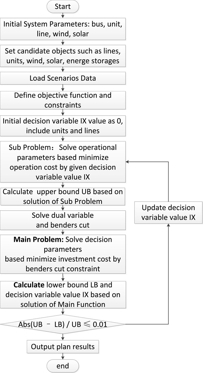
Figure 2. Co-planning model solution algorithm.

where Eq. 23 $IX$ is the investment decision variable and $F\left(IX\right)$ is the investment cost. The constraint conditions are simplified as R $\left(IX\right)\le 0$, W $\left(IX\right)\le 0,V\left(IX\right)\le \beta$, and $\beta \ge 0$. R $\left(IX\right)\le 0$ is the investment constraint, W $\left(IX\right)\le 0$ is the Benders cut when there is no feasible solution to the subproblem, and $V\left(IX\right)\le \beta$ is the Benders cut when there is an optimal solution to the subproblem. The subproblem Eq. 24 is

$V\left(IX\right)=\mathit{min}F\left(OY\right),(24)$

where $OY$ is the operating state variable and $F\left(OY\right)$ is the operating cost. The constraint conditions are simplified as $G\left(IX,OY\right)\le 0$, which is required for the normal operation of the power system.

Figure 1 presents the flowchart of the bi-level stochastic algorithm for solving the proposed model.

We compare the solution time for the single-level and bi-level models. The solution time for the single-level model is 31,324 s, and the solution time for the bi-level model is 1,758 s. The results demonstrate that the bi-level model is far more effective in increasing model solution efficiency.

4 Case study

4.1 IEEE RTS 24-bus

The IEEE-RTS 24-bus standard case is used to verify the model. The annual investment cost of power units is 180,000 yuan/MW, and the annual investment cost of lines is 500,000 yuan/km. The wind curtailment cost is 2,000 yuan/MWh. The load-shedding cost is 25,000 yuan/MWh. The total renewable energy capacity is 1,000 KW, which is distributed at 10 nodes.

The Table 1 compares the planning results of the system with different flexibility resources, where the basic plan includes both energy storage and demand response. The results show that the enhancement of the renewable energy consumption rate minimizes the operating cost of the basic plan and optimizes the overall economic cost of the basic plan.

Table 1

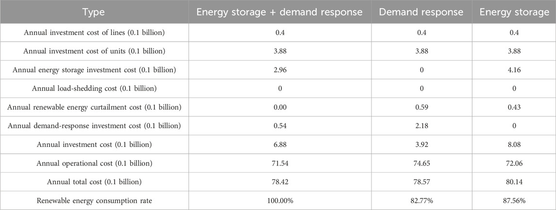
Table 1. IEEE case co-planning scheme with various flexible resources.

In order to observe the role of flexible resources in the power system, the following Figures 3−6 shows the system output graph in the four seasons of spring, summer, autumn, and winter. The load is the least from midnight to dawn, and during this time, the wind power consumption capacity is insufficient; thus, energy storage charge is required. Moreover, during noon, when the wind and solar output is large, energy storage charge also exists. From nightfall to midnight, the load is high and requires energy storage discharge, which decreases the load peak demand through demand-side response. When there are no flexible resources, curtailment of renewable energy appears due to insufficient system flexibility.

Figure 3

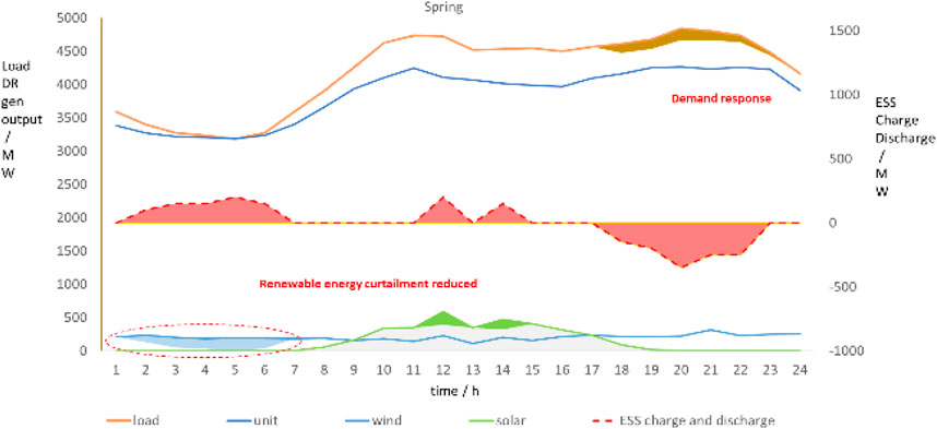
Figure 3. IEEE case spring scenario generators/load graph.

Figure 4

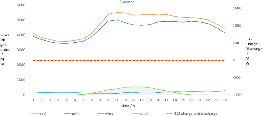
Figure 4. IEEE case summer scenario generators/load graph.

Figure 5

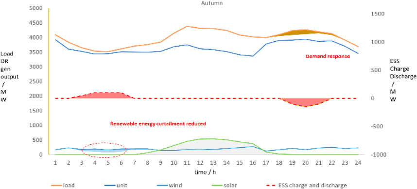
Figure 5. IEEE case autumn scenario generators/load graph.

Figure 6

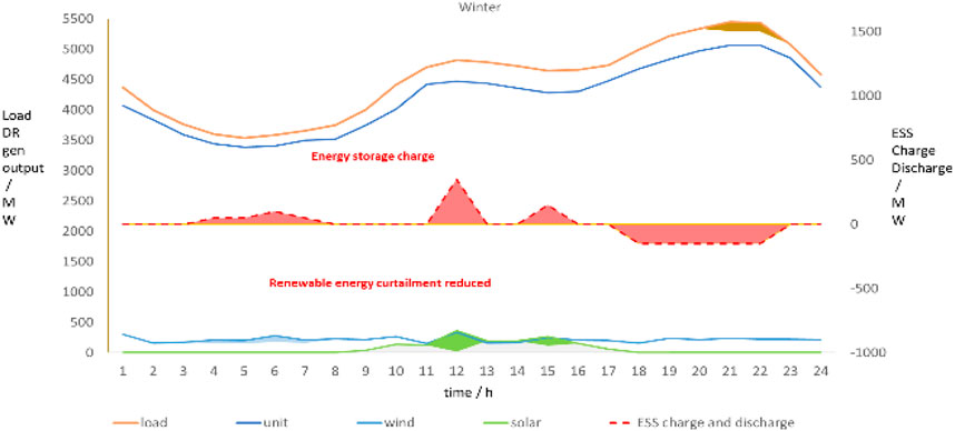
Figure 6. IEEE case winter scenario generators/load graph.

4.2 Real case study in China

The real case is a large-scale 500-kV power grid in China with a basic year and a planning year. Table 2 shows the 500-kV network real-case boundary, Table 3 shows planning parameters. In this case, wind power is equivalent to 12 nodes, and photovoltaic is equivalent to 14 nodes. At the same time, each node supports demand-side response, and the energy storage capacity to be built is 100 MW.

Table 2

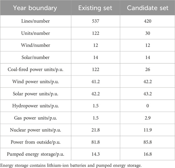
Table 2. Network real-case boundary.

Table 3

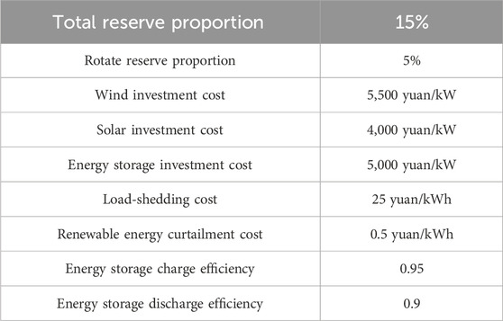
Table 3. Planning parameters.

Tables 4 and 5 show the real-case basic year and planning year flexible index calculation results.

Table 4

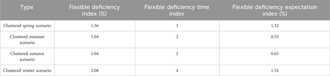
Table 4. Real-case historical year flexible indices.

Table 5

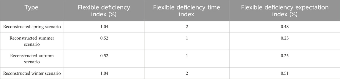
Table 5. Real-case reconstruction year flexible indices.

Table 4 is based on historical data, with four clustered operational scenarios concerning spring, summer, autumn, and winter. The flexible deficiency index, flexible deficiency time index, and flexible deficiency expectation index are separately compared. Multi-clustered scenario flexibility increases from the basic year to the planning year.

Table 5 is based on the predicted data of the planning year, and four operational scenarios concerning spring, summer, autumn, and winter are reconstructed. The flexible deficiency index, flexible deficiency time index, and flexible deficiency expectation index are separately compared. Multi-clustered scenario flexibility increases from the basic year to the planning year. Compared to historical data of the basic year, relevant flexible indices are improved because of the involvement of flexible resources. Taking the flexible deficiency expectation index in scenario four as an example, it can be seen that the indices decrease from 1.54% in the basic year to 0.51% in the planning year, and flexible deficiency is improved.

In Figures 7–9, spring and winter show large wind curtailment, which is lack of flexibility. So, when considering flexible resources, energy storage and demand response are of high demand, especially in spring and winter.

Figure 7

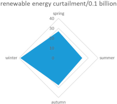
Figure 7. Real-case four-season wind curtailment with no flexible resources.

Figure 8

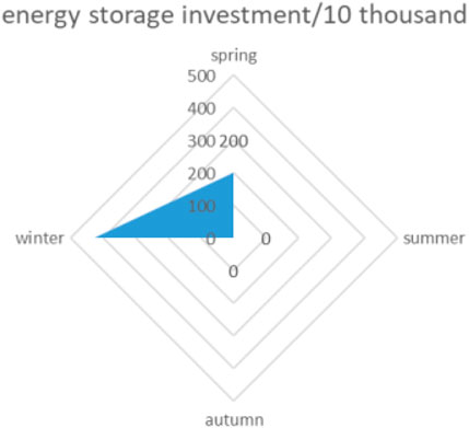
Figure 8. Real-case four-season energy storage investment cost.

Figure 9

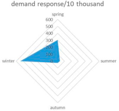
Figure 9. Real-case four-season demand-response cost.

According to the Table 6, when wind and solar installed capacity increases, energy storage increases to store more energy in the renewable energy-abundant time span, and the demand-response cost increases to respond to the load peak time span. With the increase in wind and solar installed capacity, the power supply demand of traditional units decreases, so the investment cost of traditional units also decreases. However, the increase in demand for renewable energy consumption will lead to an increase in energy storage and demand-side response, so the investment cost will also increase. Meanwhile, with the increase in wind and solar installed capacity and renewable energy generation, the fuel cost of traditional units will be reduced, so the operating cost will be reduced. According to the wind and solar installed capacity sensitivity analysis, the economic cost will increase when installing more wind and solar systems.

Table 6

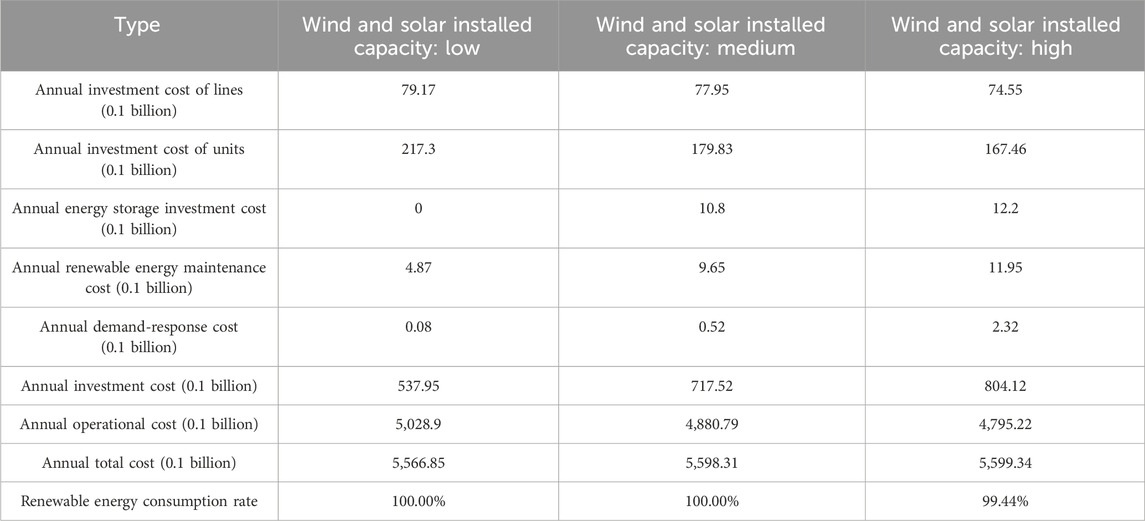
Table 6. Co-planning scheme with various wind and solar installed capacities.

The Table 7 above shows that when considering energy storage and demand responses, the investment cost is more when only considering the demand response, but it is less when only considering energy storage. Meanwhile, when considering energy storage and demand response, the operational cost is relatively lower; this is because with flexible resources involved, flexibility is ensured. When not considering energy storage or demand response, flexibility decreases, and the operational cost is more. So, the total cost is optimal when simultaneously considering energy storage and demand response.

Table 7

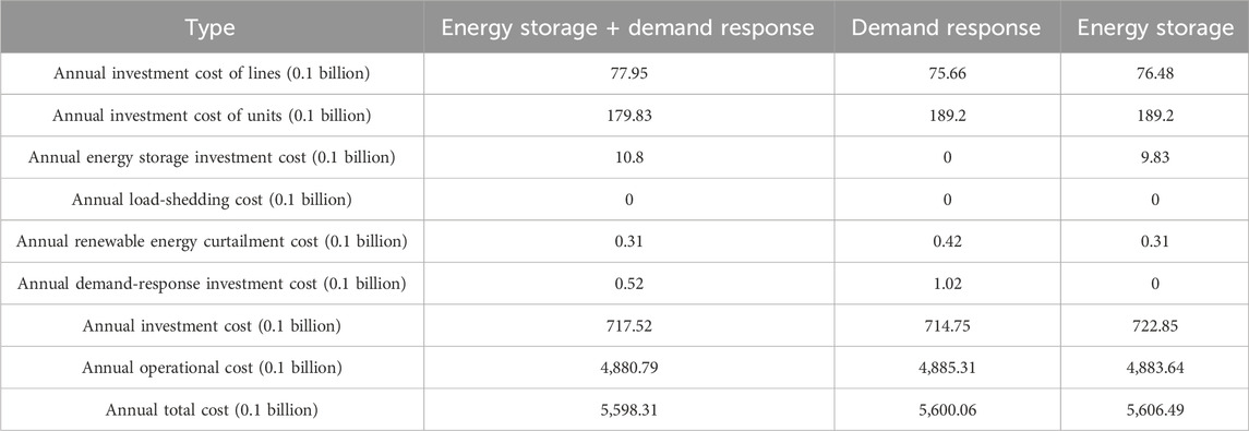
Table 7. Real-case co-planning scheme with various flexible resources.

In the above Figures 10−13, scenario generators and load graphs of the four seasons are shown to reflect unit flexible deficiency and renewable energy curtailment. When renewable energy output is high, energy storage charge is of priority; meanwhile, energy storage discharges under low renewable energy output and heavy load. While demand response is used when the load is heavy, the demand response is used at this time scale to increase system flexibility.

Figure 10

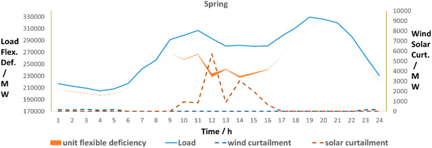
Figure 10. Spring scenario generators/load graph.

Figure 11

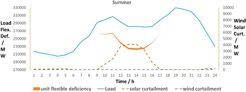
Figure 11. Summer scenario generators/load graph.

Figure 12

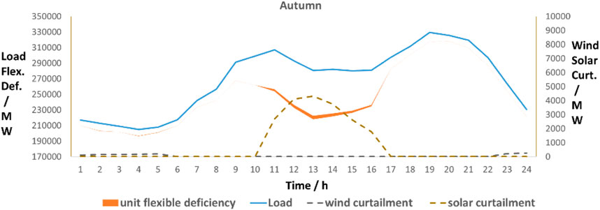
Figure 12. Autumn scenario generators/load graph.

Figure 13

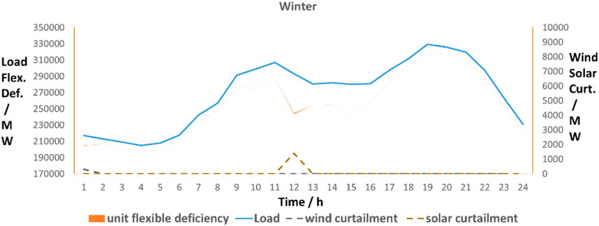
Figure 13. Winter scenario generators/load graph.

The above Table 8 separately refers to basic load *1.1, basic load, and basic load *0.7 sensitivity. With load increase, the annual demand response cost increase from basic load case 0.052 billion to basic load *1.1 case 22.69 billion. It can be seen that when the load demand decreases, the new construction cost and total economic cost of the lines and traditional units also decrease. Meanwhile, the cost of energy storage and demand-side response also decreased, indicating that the system demand for flexible resources has decreased, and the renewable energy consumption has also decreased.

Table 8

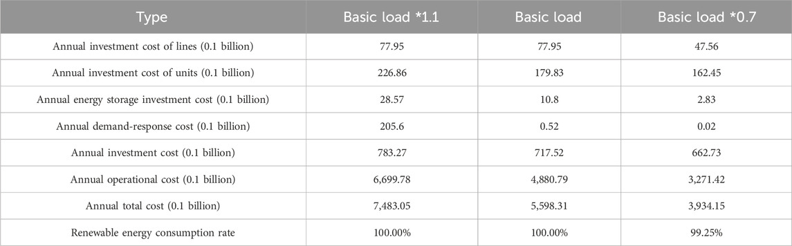
Table 8. Co-planning scheme of various load cases.

5 Conclusion

In the context of global warming and carbon emissions, this paper first proposes a generation–network–load–energy storage co-planning model. The bi-level planning of the continuous-time GNLS co-planning model is done with the objective of reducing cost and increasing renewable energy consumption. The model is comprehensive and valuable in industrial applications. A confidence-based uncertainty method is also proposed. The method applies wind and solar power output scenario cluster and reconstruction to the GNLS co-planning model. The proposed method is validated using the IEEE RTS 24-bus test system and a real-case system. It is concluded that the planning model could effectively improve the renewable energy consumption rate, and the total cost decreases to 559.8 billion. All the indices are improved in the planning year. With load increase, from the flexibility perspective, energy storage and demand response increase as a consequence.

Data availability statement

The original contributions presented in the study are included in the article/Supplementary Material; further inquiries can be directed to the corresponding author.

Author contributions

SM: writing–original draft and writing–review and editing. LL: conceptualization, visualization, and writing–review and editing. HC: resources, supervision, and writing–review and editing.

Funding

The author(s) declare that no financial support was received for the research, authorship, and/or publication of this article.

Conflict of interest

The authors declare that the research was conducted in the absence of any commercial or financial relationships that could be construed as a potential conflict of interest.

Publisher’s note

All claims expressed in this article are solely those of the authors and do not necessarily represent those of their affiliated organizations, or those of the publisher, the editors, and the reviewers. Any product that may be evaluated in this article, or claim that may be made by its manufacturer, is not guaranteed or endorsed by the publisher.

References

Abdin, A. F., Caunhye, A., Zio, E., and Cardin, M. A. (2022). Optimizing generation expansion planning with operational uncertainty: a multistage adaptive robust approach. Appl. Energy 306, 118032. doi:10.1016/j.apenergy.2021.118032

CrossRef Full Text | Google Scholar

Abdin, I. F., and Zo, E. (2018). An integrated framework for operational flexibility assessment in multi-period power system planning with renewable energy production. Appl. Energy 222, 898–914. doi:10.1016/j.apenergy.2018.04.009

CrossRef Full Text | Google Scholar

Chen, B., Liu, T., Liu, X., Nan, L., Wu, L., et al. (2018). A Wasserstein distance-based distributionally robust chance-constrained clustered generation expansion planning considering flexible resource investments. IEEE Trans. Power Syst. 38 (6), 5635–5647. doi:10.1109/tpwrs.2022.3224142

CrossRef Full Text | Google Scholar

Hamidpour, H., Aghaeij, P., Dehghan, S., and Niknam, T. (2019). Flexible, reliable, and renewable power system resource expansion planning considering energy storage systems and demand response programs. IET Renew. Power Gener. 13 (11), 1862–1872. doi:10.1049/iet-rpg.2019.0020

CrossRef Full Text | Google Scholar

Han, S., Qiao, Y. H., Yan, J., Liu, Y. q., Li, L., and Wang, Z. (2019). Mid-to-long term wind and photovoltaic power generation prediction based on copula function and long short-term memory network. Appl. Energy 239 (4), 181–191. doi:10.1016/j.apenergy.2019.01.193

CrossRef Full Text | Google Scholar

Jin, C., Ren, D., Xiao, J., et al. (2021). Optimization planning on power system supply-grid-storage flexibility resource for supporting the “carbon neutrality” target of China. Electr. Power 54 (8), 164–174.

Google Scholar

Li, Y. H., Wang, J. X., and Ding, T. (2023b). Clustering-based chance-constrained transmission expansion planning using an improved benders decomposition algorithm. IET Generation, Transmission and Distribution. IEEE Trans. Power Syst. 38 (6), 935–946.

Google Scholar

Li, Z., Wu, L., Wang, P., et al. (2023a). Risk-averse coordinated operation of a multi-energy microgrid considering voltage/var control and thermal flow: an adaptive stochastic approach. IEEE Trans. Smart Grid 12 (5), 3914–3927. doi:10.1109/tsg.2021.3080312

CrossRef Full Text | Google Scholar

Li, Z., Wu, L., Xu, Y., et al. (2021). Risk-averse coordinated operation of a multi-energy microgrid considering voltage/var control and thermal flow: an adaptive stochastic approach. IEEE Trans. Smart Grid 12 (5), 3914–3927. doi:10.1109/tsg.2021.3080312

CrossRef Full Text | Google Scholar

Li, Z., Wu, L., Xu, Y., and Zheng, X. (2022). Stochastic-weighted robust optimization based bilayer operation of a multi-energy building microgrid considering practical thermal loads and battery degradation. IEEE Trans. Sustain. Energy 13 (2), 668–682. doi:10.1109/tste.2021.3126776

CrossRef Full Text | Google Scholar

Li, Z., Xu, Y., Wu, L., and Zheng, X. (2020). A risk-averse adaptively stochastic optimization method for multi-energy ship operation under diverse uncertainties. IEEE Trans. Power Syst. 36 (3), 2149–2161. doi:10.1109/tpwrs.2020.3039538

CrossRef Full Text | Google Scholar

Li, Z., Yang, P., Zhao, Z., and Lai, L. L. (2024). Retrofit planning and flexible operation of coal-fired units using stochastic dual dynamic integer programming. IEEE Trans. Power Syst. 39 (1), 2154–2169. doi:10.1109/tpwrs.2023.3243093

CrossRef Full Text | Google Scholar

Liu, D. D., Cheng, H. Z., Liu, J., et al. (2019). Review and prospects of robust transmission expansion planning. Power Syst. Technol. 43 (01), 135–143.

Google Scholar

Liu, J., Tang, Z., Zeng, P., Li, Y., and Wu, Q. (2022a). Distributed adaptive expansion approach for transmission and distribution networks incorporating source-contingency-load uncertainties. Int. J. Electr. Power and Energy Syst. 136, 107711. doi:10.1016/j.ijepes.2021.107711

CrossRef Full Text | Google Scholar

Liu, J., Tang, Z., Zeng, P., Li, Y., and Wu, Q. (2022b). Fully distributed second-order cone programming model for expansion in transmission and distribution networks. IEEE Syst. J. 16 (4), 6681–6692. doi:10.1109/jsyst.2022.3154811

CrossRef Full Text | Google Scholar

Qiu, J., Zhao, J., and Dong, Z. Y. (2017). Probabilistic transmission expansion planning for increasing wind power penetration. IET Renew. Power Gener. 11 (6), 837–845. doi:10.1049/iet-rpg.2016.0794

CrossRef Full Text | Google Scholar

Rintamäki, T., Oliveira, F., Afzal, S., and Salo, A. (2024). Achieving emission-reduction goals: multi-period power-system expansion under short-term operational uncertainty. IEEE Trans. Power Syst. 39 (1), 119–131. doi:10.1109/tpwrs.2023.3244668

CrossRef Full Text | Google Scholar

Saeed, P., Amir, A., and Wei, P. (2021). Flexibility-constraint integrated resource planning framework considering demand and supply side uncertainties with high dimensional dependencies. Int. J. Electr. Power Energy Syst. 133 (5), 117–223.

Google Scholar

Wang, J., Li, Q., Wang, X., et al. (2020b). A generation-expansion planning method for power systems with large-scale new energy. Proc. CSEE 40 (10), 3114–3123.

Google Scholar

Wang, Y., Lou, S., Wu, Y., Lv, M., and Wang, S. (2019). Coordinated planning of transmission expansion and coal-fired power plants flexibility retrofits to accommodate the high penetration of wind power. Transm. Distribution 13 (20), 4702–4711. doi:10.1049/iet-gtd.2018.5182

CrossRef Full Text | Google Scholar

Wang, Y., Lou, S., Wu, Y., and Wang, S. (2020a). Flexible operation of retrofitted coal-fired power plants to reduce wind curtailment considering thermal energy storage. IEEE Transaction Power Syst. 35 (2), 1178–1187. doi:10.1109/tpwrs.2019.2940725

CrossRef Full Text | Google Scholar

Yang, X., Mu, G., Chai, G., et al. (2021). Source-storage-grid integrated planning considering flexible supply-demand balance. Power Syst. Technol. 44 (9), 3238–3245.

Google Scholar

Yi, J. H., Rachid, C., Mario, P., et al. (2020). Optimal Co-planning of ESSs and line reinforcement considering the dispatchability of active distribution networks. IEEE Transaction Power Syst. 38 (3), 1178–1187.

Google Scholar

Zhang, C., Cheng, H., Liu, L., Zhang, H., and Zhang, X. (2020). Coordination planning of wind farm, energy storage and transmission network with high-penetration renewable energy. Int. J. Electr. Power and Energy Syst. 120, 105944. doi:10.1016/j.ijepes.2020.105944

CrossRef Full Text | Google Scholar

Zhang, H., Cheng, H. Z., Zeng, P. L., et al. (2017). Overview of transmission network expansion planning based on stochastic optimization. Power Syst. Technol. 41 (10), 3121–3129.

Google Scholar

Zhang, S., Gu, W., Lu, S., Yao, S., Zhou, S., and Chen, X. (2021). Dynamic security control in heat and electricity integrated energy system with an equivalent heating network model. IEEE Trans. Smart Grid 12 (6), 4788–4798. doi:10.1109/tsg.2021.3102057

CrossRef Full Text | Google Scholar

Zhang, S., Gu, W., Wang, J., Zhang, X. P., Meng, X., Lu, S., et al. (2023). Steady-state security region of integrated energy system considering thermal dynamics. IEEE Trans. Power Syst. Early access, 1–15. doi:10.1109/tpwrs.2023.3296080

CrossRef Full Text | Google Scholar

Zhang, X., and Conejo, A. J. (2018). Robust transmission expansion planning representing long- and short-term uncertainty. IEEE Trans. Power Syst. 33 (2), 1329–1338. doi:10.1109/tpwrs.2017.2717944

CrossRef Full Text | Google Scholar

Zhuo, Z., Zhang, N., Xie, X., et al. (2021). Key technologies and developing challenges of power system with high proportion of renewable energy. Automation Electr. Power Syst. 45 (9), 171–191.

Google Scholar

Zhuo, Z. Y., Du, E., Zhang, N., Kang, C., Xia, Q., and Wang, Z. (2020). Incorporating massive scenarios in transmission expansion planning with high renewable energy penetration. IEEE Transaction Power Syst. 35 (2), 1061–1074. doi:10.1109/tpwrs.2019.2938618

CrossRef Full Text | Google Scholar

Ziaee, O., Alizadeh Mousavi, O., and Choobineh, F. (2018). Co-optimization of transmission expansion planning and TCSC placement considering the correlation between wind and demand scenarios. IEEE Trans. Power Syst. 33 (1), 206–215. doi:10.1109/tpwrs.2017.2690969

CrossRef Full Text | Google Scholar