Optimization method of time-of-use electricity price for the cost savings of power grid investment

The concept of time-of-use (TOU) electricity pricing is widely recognized as a key strategy to bridge the gap between electricity availability and consumption, enhance the efficiency of electricity, and refine the patterns of electricity usage. Nonetheless, the existing policy on pricing electricity based on TOU electricity pricing is missing a theoretical approach that evaluates the load properties and the advantages of investing in the power grid. Consequently, the article suggests a method for optimizing electricity prices based on TOU electricity pricing to reduce the costs associated with investing in power grids. Initially, a model for optimizing electricity prices based on TOU electricity pricing is developed, offering support for the pricing strategy of the power grid; Subsequently, a method for dividing TOU electricity pricing using the Gaussian Mixture Module (GMM) clustering algorithm is introduced, offering theoretical backing for the creation of such pricing strategies; Following this, a detailed optimization approach for electricity pricing of electricity TOU electricity pricing is suggested, along with taking into account the benefits of grid investments and the power grid’s load properties, the formulation of the electricity pricing strategy for TOU electricity pricing; Ultimately, this approach is corroborated by the Chongqing power system in China, aiming to minimize disparities in peak load valleys and enhance the advantages of grid investments, thereby offering technical assistance for the scientific determination of TOU electricity pricing.

1 Introduction

The electric power sector has seen swift growth in recent times, with studies indicating that by 2022, societal electricity usage reached 8.64 trillion kWh, marking a 3.6% rise from the previous year. Anticipations are high for a more robust increase in electricity demand in 2023, with societal electricity usage projected to climb to 9.15 trillion kWh, marking a roughly 6% growth from 2022 (SUN, 2023). Yet, as the demand for electricity rises, the disparity between its supply and demand increasingly becomes evident. To bridge the gap between supply and demand and ensure power grid companies invest effectively and precisely, enhancing the TOU electricity pricing system is critically important (HAN, 2021).

The TOU electricity pricing is a widely used tool for managing demand. An effective TOU electricity pricing strategy can motivate active user engagement in responding to demand, leading to optimal shaving and filling of valleys. Conversely, an illogical policy on TOU electricity pricing will result in additional degradation of load properties, challenges in recouping the grid company’s investment expenses, and other issues. Numerous research efforts have focused on refining the strategy for TOU pricing electricity, primarily encompassing two key elements: the period division of TOU electricity prices and the determination of these electricity prices.

The period division of TOU electricity price, being a crucial cornerstone and pivotal aspect of TOU electricity pricing strategy, has a direct impact on its execution. Current techniques for segmenting the TOU electricity price period primarily encompass empirical analysis, factor analysis, affiliation function method, and cluster analysis. The method of empirical analysis involves segmenting time periods among electric power personnel, integrating their individual work expertise and professional acumen (Min et al., 2005). While this technique is straightforward and simple to implement, it falls short in scientific grounding and is heavily swayed by personal volition. The method of factor analysis involves examining and tallying the public determinants in past load data, followed by segmenting the time frame according to the load’s comprehensive attributes (LIU, 2006). This approach merges scientific statistical analysis techniques with conventional empirical methods, yet human elements continue to affect the selection of factors, lacking theoretical backing. The fundamental concept behind the affiliation function approach involves determining the highest and lowest affiliations for each time frame on the load curve, utilizing the affiliation function in line with the standard load curve, and calculating the outcomes of dividing the time period according to the affiliation threshold. In contrast to the empirical and factor analysis methods, this approach is straightforward, effective, and scientifically grounded. However, its ultimate division outcomes hinge on the chosen affiliation threshold, making it challenging to accurately ascertain the peak and valley time interval’s demarcation points (DING et al., 2001a; XING et al., 2007; Chong, 2019). The method of cluster analysis involves categorizing data into various groups, each containing similar elements, by analyzing the inherent correlation among data (Ravi et al., 2022). This technique is prevalent in the segmentation of TOU electricity pricing periods due to its resistance to subjective biases and its ability to thoroughly explore correlations across time intervals (QIAO, 2011; DONG and LIN, 2019; JIANG et al., 2021; Lei et al., 2021). The essence of these methodologies lies in choosing a clustering algorithm that aligns with the data set’s features, and the process of selecting an appropriate clustering algorithm based on the load data’s attributes requires further in-depth investigation.

Beyond the period division of TOU electricity pricing, the determination of these electricity prices directly influences their efficiency in directing the modification of load properties. The fine-tuning of TOU electricity prices can be tailored to either the cost of supply or the response to demand. In reference Li (2007), Gao et al. (2019), Zhongfu et al. (2019), construct time-of-use price optimization model based on power supply cost by analyzing the relationship between feed-in price or marginal cost of transmission and distribution and load characteristics; In reference RUAN et al. (2012), YU et al. (2012), Wang et al. (2013), ZHAO et al. (2013), LI et al. (2015), ZHANG and YU (2018) construct time-of-use price optimization model based on demand response by analyzing consumer response behavior to price signal. On the basis of the above models, references Yang et al. (2013), CUI et al. (2018) design reasonable time-of-use pricing to construct corresponding optimization models. In reference HUANG et al. (2023), considering the planning cost and generation cost of source network uncertainty and the uncertainty of load side user response, a two-layer optimization model of peak-valley period and peak-valley price is proposed to optimize peak-valley period division and peak-valley price. Nonetheless, the aforementioned techniques solely focus on the operational advantages of the grid company’s TOU electricity pricing approach, neglecting the investment gains of the grid company. This narrows the optimization scope for TOU electricity pricing, leading to a peak-valley price difference in the existing TOU electricity pricing, making it challenging to fully exploit the user demand response potential. Indeed, the grid company’s scientifically sound and sensible approach to TOU pricing electricity significantly outweighs its operational advantages. This strategy not only cuts down the investment expenses of the grid company but also fine-tunes the user’s electricity usage patterns. Consequently, examining the model for optimizing TOU electricity prices is crucial, considering the enhancement of load properties and the grid’s investment advantages.

Addressing the aforementioned issues, this document introduces a method for optimizing TOU electricity prices, taking into account the grid’s investment advantages, thereby enhancing the grid’s investment value and load properties through the application of the TOU electricity pricing approach. Initially, a model for optimizing TOU electricity prices and its investment advantages is developed by examining user load transfer traits and the advantages for both the grid company and its users. Subsequently, a method for dividing of TOU electricity price period, utilizing the GMM algorithm, is introduced to offer technical assistance. Ultimately, a thorough optimization approach for both the TOU electricity price and its division is suggested, and its efficacy is confirmed through a provincial power system in China.

2 Time-of-use price optimization model considering power grid investment benefit

The TOU electricity pricing exerts a guiding influence on users’ electricity consumption behavior. The implementation of TOU electricity pricing has the potential to modify the user load curve, thereby reducing the investment cost of the power grid. This paper aims to optimize the user load curve, reduce the investment cost of the power grid, and minimize the electricity expenses for users by employing a user response model that considers load transfer characteristics. The text also presents a cost-benefit sharing approach for power grid investment and introduces a TOU electricity price optimization model that takes into account the investment benefits of the power grid.

2.1 User response model considering load transfer characteristics

The TOU electricity pricing mechanism influences the shifting of electricity load. By implementing user load transfer, it is possible to make significant improvements to load characteristics and optimize the user load curve. The paper employs the classical load transfer model to effectively characterize the user load as a piecewise linear function, which is segmented into the dead zone, linear zone, and saturated zone (LIN, 2015). In the region of low demand, the disparity in electricity prices is minimal, thereby failing to elicit a significant response from users. Conversely, in the linear region, the user’s reaction is expected to exhibit a positive correlation with the extent of the electricity price differential. However, in the saturated region, users are anticipated to cease responding to further increases in the price differential due to the restricted capacity for load transfer, thereby reaching the limit of user responsiveness.

According to the aforementioned theory, the day is segmented into peak, normal, and valley periods. According to the division of periods, the load transfer models can be categorized into peak period to normal period, peak period to valley period, and normal period to valley period, as illustrated in Figure 1.

FIGURE 1

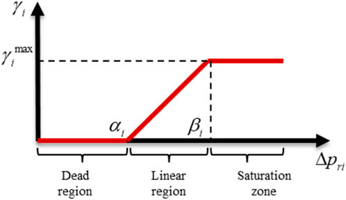
FIGURE 1. Model of Load transfer.

The function expression for the load transfer model is as follows:

${\gamma }_i=\left\{\begin{array}{l}0,0\le \Delta p_{ri}\le {\alpha }_i\\ \Delta p_{ri}{\gamma }_i^{\max }/\left({\beta }_i-{\alpha }_i\right),{\alpha }_i<\Delta p_{ri}\le {\beta }_i\\ {\gamma }_i^{\max },\Delta p_{ri}>{\beta }_i\end{array}\right.(1)$

In the given equation, $i=1,2,3$ represent the peak period to the normal period, the peak period to the valley period, and the normal period to the valley period. Additionally, ${\gamma }_i$ represents the load transfer rate, $\Delta {\mathrm{P}}_{ri}$ represents the electricity price difference, ${{\gamma }_i}^{\max }$ represents the maximum value of the load transfer rate, ${\alpha }_i$ and ${\beta }_i$ respectively represents the upper and lower limits of the price difference in the linear region of the load transfer model.

The description of the load transfer model between each period is now complete, as represented by Eq. 1. Following the price optimization, it is necessary to consider the transfer of the load. Consequently, by the user load transfer characteristic model presented above, Eq. 2 illustrates the load value for each period under the optimized TOU electricity price strategy (Domingo et al., 2011).

$p_{\text{load}\_i}=\left\{\begin{array}{l}{p}_{\text{load}\_i0}-{\gamma }_1{\overline{p}}_{\text{load}\_f0}-{\gamma }_2{\overline{p}}_{\text{load}\_f0},i\in T_1\\ p_{\text{load}\_i0}-{\gamma }_3{\overline{p}}_{\text{load}\_p0}+{\gamma }_1{\overline{p}}_{\text{load}\_f0},i\in T_2\\ p_{\text{load}\_i0}+{\gamma }_2{\overline{p}}_{\text{load}\_f0}+{\gamma }_3{\overline{p}}_{\text{load}\_p0},i\in T_3\end{array}\right.(2)$

In the equation: $p_{\text{load}\_i0}$ and $p_{\text{load}\_i}$ are the load of period $i$ under the TOU electricity price before and after optimization; ${\overline{p}}_{\text{load}\_f0}$ and ${\overline{p}}_{\text{load}\_p0}$ are the average load of the peak period and the normal period before the TOU electricity price optimization; T1, T2 and T3 represent the collection of peak, normal and valley periods, respectively.

In the given equation, $p_{\text{load}\_i0}$ and $p_{\text{load}\_i}$ represent the load during the period $i$ under the TOU electricity price before and after optimization, ${\overline{p}}_{\text{load}\_f0}$ and ${\overline{p}}_{\text{load}\_p0}$ represent the average load during the peak and normal periods before the TOU electricity price optimization. T1, T2, and T3 denote the sets of peak, normal, and valley periods, respectively.

2.2 Time-of-use price optimization model considering power grid investment benefit

To achieve the investment benefits of the power grid and reduce users’ electricity costs, this section aims to minimize peak load and peak-valley differences in load by considering load transfer characteristics in the user response model Eqs 1, 2. The model also incorporates user-side and grid-side income as constraints and constructs Eqs 1–14 for the optimization of TOU electricity pricing.

① Objective function:

$\min \left[w_1\left(\max {\mathbf{P}}_{\text{load}}\right)+w_2\left(\max {\mathbf{P}}_{\text{load}}-\min {\mathbf{P}}_{\text{load}}\right)\right](3)$

${\mathbf{P}}_{\text{load}}\triangleq \left\{\forall p_{\text{load}\_i},i\in T_1\cup T_2\cup T_3\right\}(4)$

In the given equation, ${\mathbf{P}}_{\text{load}}$ represents the load vector under the optimized TOU electricity price, where the symbol $\triangleq$ is “equivalent to” indicates that the right-hand symbol is equivalent to the left-hand equation. Both w1 and w2 serve as weight coefficients. The first component of the objective function denotes the load peak value under the optimized price, while the second component represents the load peak-valley difference under the optimized price. By modifying the weight coefficient, a balance is achieved between the two objectives.

② Constraint conditions:

 1) Grid-side revenue constraints are implemented to prevent a decrease in the revenue of the grid company due to the adjustment of the TOU electricity price strategy. This is achieved by setting the condition that under the optimized TOU electricity price strategy, the grid company’s revenue from the sale of electricity should not be lower than the revenue generated before the optimization, as represented by Eqs 5–7.

$E_A\ge E_0(5)$

$E_A={\displaystyle \sum _{i\in I}}{\lambda }_i{p}_{\text{load}\_i}-{\displaystyle \sum _{i\in I}}{h}_i{p}_{\text{load}\_i}(6)$

$E_0={\displaystyle \sum _{i\in I}}{\lambda }_{i0}{p}_{\text{load}\_i0}-{\displaystyle \sum _{i\in I}}{h}_i{p}_{\text{load}\_i0}(7)$

Where $E_0$ and $E_A$ are the power company’s revenue from electricity sales before and after the implementation of TOU electricity price optimization. ${\mathrm{\lambda }}_{\mathrm{i}0}$ and ${\mathrm{\lambda }}_{\mathrm{i}}$ are TOU electricity prices under period $i$ before and after optimization. $h_i$ is the marginal cost of power generation of the system in the period $i$. Additionally, the study considers the concatenated set of all periods, i.e., $I=T_1\cup T_2\cup T_3$.

 2) Customer-side benefit constraint: To prevent an increase in the cost of electricity for the customer resulting from changes in electricity prices, it is necessary to establish that following the TOU electricity price optimization, the average cost of electricity to the customer does not exceed the pre-optimization cost, as represented by Eq. 8:

$\frac{{\displaystyle \sum _{i\in I}}{\lambda }_i{p}_{\text{load}\_i}}{{\displaystyle \sum _{i\in I}}{p}_{\text{load}\_i}}<\frac{{\displaystyle \sum _{i\in I}}{\lambda }_{i0}{p}_{\text{load}\_i0}}{{\displaystyle \sum _{i\in I}}{p}_{\text{load}\_i0}}(8)$

 3) The price constraint for each period is established to prevent the irrationality of the optimized TOU electricity price strategy, which could exacerbate the deterioration of load characteristics. Specifically, it is stipulated that the price of electricity in the peak period under the optimized TOU electricity pricing is higher than the price of electricity in the weekday period, and the price of electricity in the weekday period is higher than the price of electricity in the valley period, as expressed in Eq. 9.

${\lambda }_f>{\lambda }_p>{\lambda }_g(9)$

The optimized electricity prices for the peak hour, the usual hour, and the valley hour are denoted by ${\mathrm{\lambda }}_{\mathrm{f}}$ , ${\mathrm{\lambda }}_{\mathrm{p}}$ and ${\mathrm{\lambda }}_{\mathrm{g}}$ respectively.

 4) The constraint on the difference between peak and valley prices is essential to maintain the rationality of the TOU electricity pricing strategy. It is typically limited to a specific range, as represented by Eq. 10.

${\tau }_{\max }>\frac{{\lambda }_f}{{\lambda }_g}>{\tau }_{\min }(10)$

Where ${\tau }_{\max }$ and ${\tau }_{\min }$ represent the upper and lower limits of the peak-to-valley electricity price scaling factor.

 5) Generation cost constraint: To prevent financial losses for the grid company due to the introduction of the new TOU electricity pricing strategy, it is necessary to establish that the optimized TOU electricity price exceeds the marginal cost of electricity generation, as represented by Eq. 11:

${\lambda }_i\ge h_i(11)$

 6) Constraints associated with peak loads and peak-to-valley differences: The capacity of the equipment is directly affected by peak loads, which in turn influences grid investment. To reduce grid investment, it is important to ensure that the load peak following TOU electricity price optimization does not surpass the peak before optimization, as indicated in Eq. 12. Moreover, a greater peak-to-valley load difference results in reduced operational efficiency and economic performance of the power system. The condition is stipulated that the peak-to-valley difference after the optimization of TOU electricity pricing must not surpass the peak-to-valley difference before optimization, as denoted by Eq. 13.

$\max {\mathbf{P}}_{\text{load}}\le \max {\mathbf{P}}_{\text{load}0}(12)$

$\max {\mathbf{P}}_{\text{load}}-\min {\mathbf{P}}_{\text{load}}\le \max {\mathbf{P}}_{\text{load}0}-\min {\mathbf{P}}_{\text{load}0}(13)$

${\mathbf{P}}_{\text{load}0}\triangleq \left\{\forall p_{\text{load}\_i0},i\in T_1\cup T_2\cup T_3\right\}(14)$

Where ${\mathbf{P}}_{\text{load}0}$ represents the load vector be located in the context of TOU electricity pricing before any optimizations? Equations 1–14 depict essential models for price optimization, which are capable of reducing price peaks and filling troughs.

Furthermore, the exclusion of grid investment costs in Eq. 5 limits the optimization space for TOU electricity prices to only the grid company’s power sales revenue. This limitation hinders the achievement of enhanced load characteristics, reduced grid company investment costs, and lower electricity consumption costs for customers. Therefore, to address the aforementioned issues, this section enhances Eq. 5 and formulates a model for sharing the benefits of grid investment. The objective is to minimize the grid company’s investment expenses by devising a viable TOU electricity pricing strategy. The goal is to minimize the investment expenditure of the power grid company by designing a feasible time-of-use electricity price strategy, as shown in Eqs. 15–16. Additionally, a portion of the reduced investment costs is allocated to benefit the users, thereby broadening the scope for optimizing the TOU electricity pricing and achieving a mutually beneficial outcome for both the grid company and the users. The specific enhancements are outlined below:

$E_A+\left(1-\partial \right)\Delta H\ge E_0(15)$

$H_0-\Delta H=H(16)$

Where $\partial$ represent the concession coefficient, denoting the proportion of the investment cost saved by the power grid company that translates to profit for the users; $\Delta$ H represents the investment cost saved by the power grid company after the optimization of TOU electricity price; H represents the investment cost saved by the power grid company after the optimization of TOU electricity price; H0 represents the investment cost of the power grid company before the optimization of TOU electricity price.

H in Eq. 16 can be determined using Eqs 17–24 from the grid investment planning optimization model, which is widely employed in industry. This model takes into account both conventional units and each new energy field station, as outlined in (LIN, 2015).

Objective function:

$\begin{array}{c}\min H=\frac{\alpha {\left(\alpha +1\right)}^Y}{{\left(\alpha +1\right)}^Y-1}{\displaystyle \sum _{l\in N_l}}{c}_l{C}_l{L}_l+\\ {\displaystyle \sum _{y=1}^Y}{\displaystyle \sum _{t=1}^T}{\displaystyle \sum _{g=1}^{N_g}}{a}_g{P}_{f,g,t}\Delta t+{\displaystyle \sum _{y=1}^Y}{\displaystyle \sum _{t=1}^T}{\displaystyle \sum _{w=1}^{N_w}}{\chi }_w{P}_{w,t}^{*}\Delta t\end{array}(17)$

Where H represents the total cost of the grid, the first term denotes the annual equipment investment of the grid, the second term signifies the operation cost of thermal power, hydropower, and other traditional units, and the third term indicates the penalty cost of new energy sources such as abandoned wind and light. $\alpha$ represents the discount rate, $c_l$ stands for the investment cost of the line per unit of capacity per unit of length, $L_l$ represents the length of the lth branch, $a_g$ represents the offer of the $gth$ traditional unit, ${\chi }_w$ represents the penalty cost of the unit of energy abandonment, $C_l$ represents the $lth$ branch’s capacity, $P_{f,g,t}$ represents the power of the $gth$ conventional unit in the time period $t$, $P_{w,t}^{*}$ represents the amount of energy discarded by the $wth$ new energy station in the time period $t$, $N_l$ represents the set of routes to be optimized, $N_g$ and $N_w$ represent the number of conventional units and new energy stations, respectively, and Y represents the number of years of planning; T represents the total number of time periods, while $\Delta t$ represents the interval between time periods.

① Constraint conditions:

 1) Power balance constraint

${\displaystyle \sum _{g=1}^{N_g}}{P}_{f,g,t}+{\displaystyle \sum _{w=1}^{N_w}}{P}_{w,t}-{\displaystyle \sum _{n\in N_{\text{load}}}}{P}_{n,\text{load},t}=0(18)$

Where $\mathrm{t}=1,2\dots ,\mathrm{T}$; $N_{load}$ represents the set of nodes accessing the load; $P_{w,t}$ represents the actual power of the $wth$ new energy station in time period t; $P_{n,\text{load},t}$ represents the load of the nth node in time period t.

 2) Branch power constraint

$-C_{l0}<P_{l,t}<C_{l0}(19)$

Where $\mathrm{t}=1,2\dots ,\mathrm{T}$; $\mathrm{l}=1,2\dots ,\text{Nl}0$; Nl0 represent the total number of branch circuits in the grid; Cl0 represents the capacity of branch circuit l.

 3) Branch-planned capacity constraints

$C_l^{\min }\le C_l\le C_l^{\max }(20)$

Where $\in N_l$ ; $C_l^{\max }$ and $C_l^{\min }$ are the upper and lower limits of the plannable capacity of branch $l$ respectively.

 4) Conventional unit constraint

$P_{f,g,\min }\le P_{f,g,t}\le P_{f,g,\max }(21)$

$r_{g,\text{down}}\le P_{f,g,t}-P_{f,g,t-1}\le r_{g,\text{up}}(22)$

Where t = 1,2…,T; g = 1,2…,Ng; $P_{f,g,\max }$ and $P_{f,g,\min }$ represent the upper and lower limit values of the power of the $gth$ traditional unit; $r_{g,\text{up}}$ and $r_{g,\text{down}}$ represent the upper and lower limit values of the traditional unit to climb the slope, respectively.

5)  New energy station constraints

$0\le P_{w,t}\le P_{w,t,\max }(23)$

$P_{w,t}^{*}=P_{w,t,\max }-P_{w,t}(24)$

Where t = 1,2…,T; $P_{w,t,\max }$ represents the maximum generating power of the $wth$ new energy station in t period.

In summary, the model proposed in this paper is essentially a two-layer optimization model, and in the actual grid model, firstly, with Eq. 17 as the objective function and Eqs 18–24 as the constraints, the inner layer optimization model is solved to obtain the investment cost H of the grid company after the optimization of TOU electricity price and to achieve the saving of the grid investment cost. Then, we substitute it into Eq. 16 and solve the outer optimization model with Eq. 3 as the objective function and Eqs 5–16 as the constraints. The load transfer is guided to realize the “peak shaving and valley filling” of the load curve.

In summary, the model presented in this paper is fundamentally a two-layer optimization model. In the actual grid model, the inner layer optimization model is solved first, with Eq. 17 serving as the objective function and Eqs 18–24 as the constraints, to obtain the investment cost H of the grid company after optimizing the TOU electricity price and achieving savings in grid investment costs. Subsequently, the substitution is made into Eq. 16 and the outer optimization model is solved, with Eq. 3 serving as the objective function and Eqs 5–16 as the constraints. The load transfer is directed towards achieving “peak shaving and valley filling” of the load curve.

3 Time-of-use electricity price optimization approach considering grid investment efficiency

To develop a TOU electricity pricing strategy that considers the grid’s investment benefits and maximizes its effectiveness in enhancing customer load characteristics and reducing grid investment costs, this section presents a TOU electricity pricing time slot division approach based on the GMM clustering algorithm. It also integrates the TOU electricity pricing optimization model discussed in Section 1 to propose a comprehensive optimization strategy for TOU electricity prices and time slots, taking into consideration the grid’s investment benefits.

3.1 GMM clustering algorithm based time-sharing tariff time slot division method

The section proposes a time slot division method based on the GMM clustering algorithm to address issues related to objectivity and adaptability in traditional time slot division methods. This approach aims to provide technical support for the reasonable division of time-sharing tariff time slots and mitigate the influence of subjective factors on the results.

The GMM clustering relies on the probability of classification members, which falls under “soft classification.” This method does not explicitly assign members to a specific category but instead provides the probability of a member belonging to each category. The information conveyed by this approach is considerably greater than that of K-means and other “hard classification” clustering methods, resulting in improved clustering effectiveness. Additionally, GMM clustering can more effectively uncover correlations between various attributes. As a result, GMM clustering algorithms are currently extensively employed across diverse fields (DANG et al., 2015).

The GMM is derived by linearly combining multiple Gaussian distribution functions. The r-dimensional sample dataset ${\mathbf{D}}_r=\left(x_1,x_2,...,x_r\right)$ be classified into S classes, and the Gaussian mixture model, which comprises a mixture of S Gaussian distributions, is defined by an Eq. 25:

$P\left(x\right)={\displaystyle \sum _{s=1}^S}{\alpha }_{s}p\left(x|{\beta }_s\right)(25)$

$p\left(x|{\beta }_s\right)=\frac{1}{\sqrt{{\sum }_s}{\left(2\pi \right)}^{r/2}}{e}^{\left[-\frac{{\left(x-{\mu }_s\right)}^2}{2{\sum }_s}\right]}(26)$

${\displaystyle \sum _{s=1}^S}{\alpha }_s=1,0\le {\alpha }_s\le 1(27)$

Where $P\left(x\right)$ represent the probability density function of GMM; $p\left(x|{\beta }_s\right)$ represent the probability density function of the $sth$ Gaussian distribution; ${\alpha }_s$、 ${\mu }_s$、 ${\sum }_s$ represent the weight, expectation and covariance matrix of the $sth$ Gaussian distribution, respectively.

The output of a GMM consists of a sequence of probability values, and the category with the highest probability is considered as the one to which the member belongs. Determining the probability value necessitates identifying the Gaussian distribution to which the member belongs, and ensuring that the Gaussian distribution accurately represents the sample data by fitting it as closely as possible, thereby ensuring that its parameters are accurate. The Expectation-Maximization algorithm (EM) (Zanetti et al., 2015) is employed for parameter estimation of the GMM. The fundamental concept of EM is to iteratively optimize the likelihood estimation of the model distribution parameters, converging on the model parameters by repeatedly iterating until the likelihood function value reaches convergence, thereby completing the parameter estimation process. Furthermore, due to the complexity of solving the likelihood estimation function for sample data in the Gaussian mixture model, it is common to use the logarithm of the likelihood function, as shown in Eq. 28:

$\ln {\displaystyle \prod _{i=1}^r}P\left(x_i|\alpha ,\mu ,\sum \right)={\displaystyle \sum _{i=1}^r}\ln \left[{\displaystyle \sum _{s=1}^S}{\alpha }_{s}p\left(x|{\beta }_s\right)\right](28)$

The EM algorithm primarily engages in iterative parameter estimation through two steps: the E-Step (Expectation Step) and the M-Step (Maximization Step). The E-Step involves calculating the probability that each data point is generated by each Gaussian distribution using the initial values of $\alpha$、 $\mu$ 、 $\sum$ or the value obtained from the previous iteration. The M-Step entails solving and updating the model parameters based on the value obtained from the E-Step.

Based on the aforementioned theory, to achieve a precise division of time-sharing tariff periods, this section presents a method for time-sharing tariff period division based on the GMM clustering algorithm. The flowchart of this method is illustrated in Figure 2 and described below.

FIGURE 2

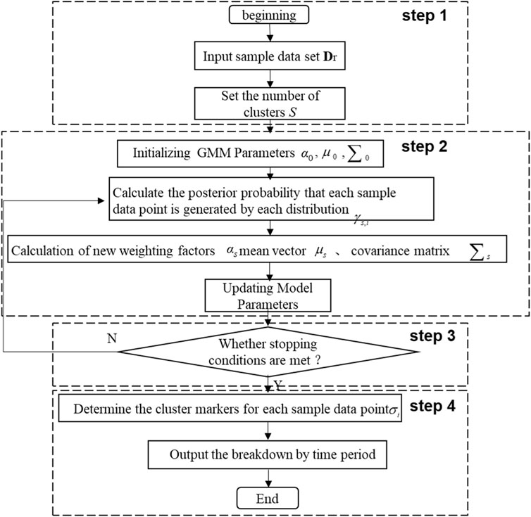
FIGURE 2. Division method of TOU price based on GMM clustering algorithm.

Step 1: First, give an r-dimensional sample set of typical daily load data ${\mathbf{D}}_r=\left(x_1,x_2,...,x_r\right)$ (e.g., one data point at 1 h intervals, a day has 24 time periods, r = 24); second, given the number of clusters S (e.g., if a day is divided into 3 time periods, peak, normal, and valley, then S = 3), the GMM consists of a mixture of S Gaussian distributions.

Step 2: First, the initial GMM parameters ${\alpha }_0$、 ${\mu }_0$、 ${\sum }_0$ are randomly given. Second, E-Step is used to calculate the posterior probability of each data sample $x_i\left(i=1,2,...,r\right)$ in the sample set ${\mathbf{D}}_r=\left(x_1,x_2,...,x_r\right)$ generated by the sth Gaussian distribution ${\gamma }_{s,i}$ as in Eq. 29. Finally, on the basis of the values obtained by E-Step, the GMM parameters are updated by M-Step as in Eqs 30–32.

Step 3: Determine whether the stopping condition is satisfied, i.e., when the maximum number of iterations is reached or the log-likelihood function Eq. 28 converges go to Step 4 to complete the estimation of the GMM parameters; otherwise, go to Step 2 to repeat E-Step and M-Step.

Step 4: First, according to the a posteriori probability ${\gamma }_{s,i}$ that the data sample $x_i\left(i=1,2,...,r\right)$ may be generated by each Gaussian distribution, we select the cluster with the largest a posteriori probability ${\gamma }_{s,i}$ as the cluster to which the time period belongs, and mark the cluster ${\sigma }_i$ as Eq. 33; second, according to the cluster marking, divide the data sample ${\mathbf{D}}_r=\left(x_1,x_2,...,x_r\right)$ set into S clusters $T_{all}=\left\{T_1,T_2,...,T_S\right\}$, and the resulting S clusters $T_{all}$ are the S classes of the time period, with the time period belonging to that class included in each class, thus completing the division of the time-sharing tariff time period.

${\gamma }_{s,i}={\alpha }_{s}p\left(x_i|{\beta }_s\right)/{\displaystyle \sum _{s=1}^S}{\alpha }_{s}p\left(x_i|{\beta }_s\right)(29)$

${\alpha }_s={\displaystyle \sum _{i=1}^r}{\gamma }_{s,i}/n,s=1,2,...,S(30)$

${\mu }_s={\displaystyle \sum _{i=1}^r}{\gamma }_{s,i}{x}_i/{\displaystyle \sum _{i=1}^r}{\gamma }_{s,i},s=1,2,...,S(31)$

${\sum }_s={\displaystyle \sum _{i=1}^r}{\gamma }_{s,i}{\left(x_i-{\mu }_s\right)}^2/{\displaystyle \sum _{i=1}^n}{\gamma }_{s,i},s=1,2,...,S(32)$

${\sigma }_i=\mathrm{argmax}{\gamma }_{s,i},i=1,2,...,r;s\in \left\{1,2,...,S\right\}(33)$

3.2 An integrated optimization strategy for time-of-day tariff prices and time slots considering grid investment efficiency

The design of a time-of-day tariff encompasses two primary components: time slot division and price determination. This subsection consolidates the time-of-day tariff price optimization model, which takes into account the grid investment benefit outlined in Section 1, and the time-of-day tariff time slot division method based on the GMM clustering algorithm discussed in Section 2.1. Furthermore, it introduces a comprehensive optimization strategy for time-of-day tariff price and time slot, considering the grid investment benefit, as depicted in Figure 3. The specific steps are outlined below:

FIGURE 3

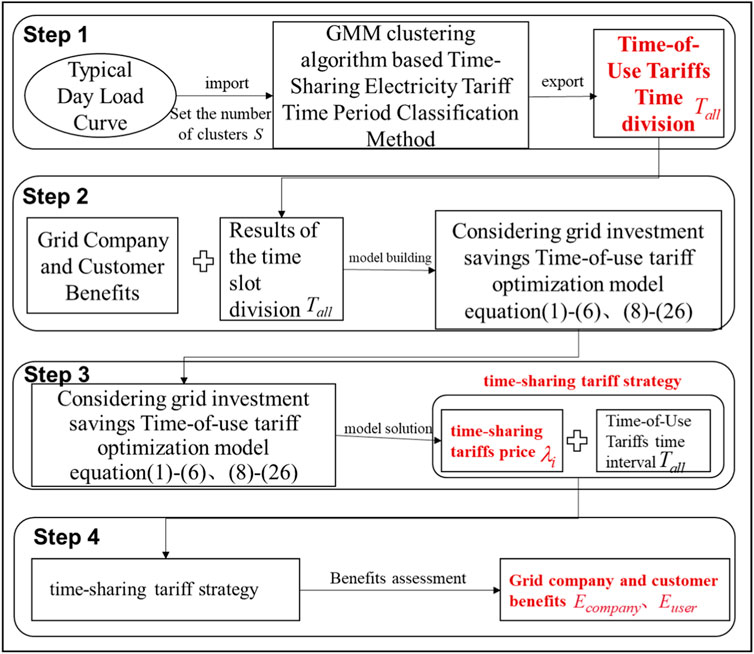
FIGURE 3. Comprehensive optimization strategy for TOU electricity price and time period considering power grid investment savings.

Step 1: First, give a typical daily load profile as input and set it to divide a day into S categories such as peak, normal, valley, etc. second, adopt the time-sharing tariff time period division method based on GMM clustering algorithm proposed in Section 2.1 to obtain S clusters $T_{all}=\left\{T_1,T_2,...,T_S\right\}$ such as peak, normal, valley, etc. where each of the clusters contains a time period belonging to the cluster, so as to realize the division of time-sharing tariff time periods.

Step 2: Based on the results of the obtained time slot division $T_{all}$ , the time slots are included in the categories of peak, normal, and valley are determined to complete the construction of the time-sharing tariff optimization model Eqs 1–4 and Eqs 6–24 proposed in this paper considering the investment benefits of the power grid.

Step 3: First, solve the time-sharing tariff price optimization model by adopting algorithms such as the out-point method (cited in the literature), and obtain the time-sharing tariff price; secondly, combine with the time slot division method obtained in step 1, and finally obtain the time-sharing tariff strategy. For example, set the number of clusters S = 3, the 24 h of the day are divided into peak hours, weekdays and valleys, then according to the results of the time division, the following time-sharing tariff strategy can be constructed. A time-of-use electricity price strategy can be constructed as shown in Eq. 34:

${\lambda }_i=\left\{\begin{array}{l}{\lambda }_f,i\in T_1\\ {\lambda }_p,i\in T_2\\ {\lambda }_g,i\in T_3\end{array}\right.(34)$

Step 4: In order to assess the impact of the designed time-sharing tariff strategy on the benefits of the grid company and users. First, calculate the grid company’s benefit $E_{\text{company}}$, the sum of the grid company’s revenue from electricity sales and the investment cost saved by the grid company after the concessions, as in Eq. 35, the larger the value, the better the grid company’s benefit; second, calculate the price of electricity per unit of the user to characterize the user’s benefit, as in Eq. 36, the larger the reduction in the price, the larger the benefit to the user.

$E_{\text{company}}=E_A+\left(1-\partial \right)\Delta Q={\displaystyle \sum _{i\in I}}{\lambda }_i{p}_{\text{load}\_i}-{\displaystyle \sum _{i\in I}}{c}_i{p}_{\text{load}\_i}+\left(1-\partial \right)\Delta Q(35)$

$E_{\text{user}}={\displaystyle \sum _{i\in I}}{\lambda }_i{p}_{\text{load}\_i}/{\displaystyle \sum _{i\in T}}{p}_{\text{load}\_i}(36)$

The above analysis culminates in the development of a time-sharing tariff strategy that takes into account the grid’s investment benefits. This strategy offers potential solutions for enhancing the load curve, reducing grid investment costs, and lowering electricity consumption expenses for users. Furthermore, through an analysis of the advantages for both the grid company and users under the optimized time-sharing tariff, this study offers insights that can inform the appropriate adjustment of future time-sharing tariffs. This adjustment is beneficial for mitigating the conflict between power supply and demand.

4 Case study/case analysis

4.1 Validation of the effectiveness of time-of-use electricity price period segmentation method based on GMM clustering algorithm

To assess the efficacy of the TOU electricity price period segmentation method proposed in this study, a set of typical daily load data from a provincial-level power system in China was selected for period segmentation, similar to that of a real power grid (DONG et al., 2023; DING et al., 2001b). The typical daily load data is depicted in Figure 4, with the number of clusters designated as S = 3, indicating the division of the 24 time periods of a day into peak periods, off-peak periods, and normal periods.

FIGURE 4

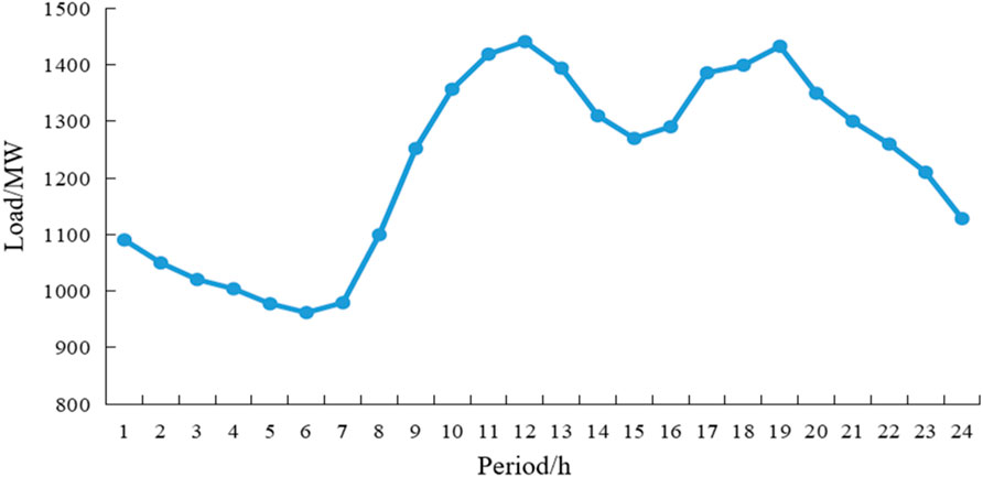
FIGURE 4. Load data of a typical day.

The existing TOU electricity pricing strategy in this province delineates time periods as follows: peak periods are from 11:00 to 17:00 and 20:00 to 22:00, off-peak periods are from 8:00 to 11:00, 17:00 to 20:00, and 22:00 to 24:00, and the valley period is from 0:00 to 8:00. Nevertheless, as depicted in Figure 4, the current time period segmentation method does not adequately capture the peak and off-peak characteristics of the province’s load. There are several instances of inconsistency, such as the load showing a significant increase at 10:00 with a high load value, yet being categorized as an off-peak period based on the current time segmentation. Similarly, at 21:00, the load demonstrates a distinct decrease but is designated as a peak period according to the current time segmentation. Consequently, it is imperative to modify the segmentation of time periods in this province.

To comprehensively illustrate the efficacy of the TOU electricity price period segmentation method based on the GMM clustering algorithm proposed in this paper, this section sets up four comparative analysis scenarios, labeled as M0 to M3.

M0: Method for segmenting the current time period.

M1: A method for segmenting TOU electricity price periods based on membership functions has been proposed (DING et al., 2001a).

M2: A method for segmenting TOU electricity price periods based on the K-means clustering algorithm (Nedal, 2011).

M3: proposes a method for segmenting TOU electricity price periods based on the Gaussian Mixture Model (GMM) clustering algorithm.

In M1 to M3, M1 denotes the conventional TOU electricity price period segmentation approach, characterized by its simplicity and efficiency, but also susceptible to significant influence from human factors. The M2 method is a traditional clustering approach frequently employed for segmenting TOU electricity price periods. It is recognized for its straightforward principles and straightforward implementation, although it has constraints regarding the types of samples to which it can be applied. The method proposed in this paper is referred to as M3.

In this section, a comparative analysis method, as cited in (QIAO, 2011), is employed to determine the percentage of peak load across various time period segments. The rationality of the proposed time period segmentation method is assessed through a comprehensive analysis. The time period divisions from M0 to M3 are presented in Table 1, while the proportion of electricity usage during peak hours within these divisions is depicted in Figure 5.

TABLE 1

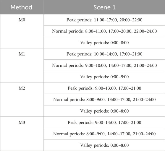
TABLE 1. Period division results of M0–M3 for TOU price.

FIGURE 5

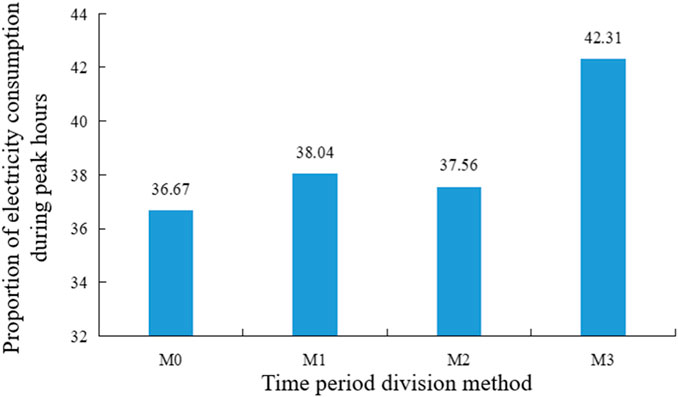
FIGURE 5. Proportion of electricity consumption during peak hours for the four methods of M0–M3.

The comparison of the proposed TOU electricity price period segmentation method M3 with M1 and M2, based on the results obtained from Table 1, yields the following observations: In the time period segmentation result of M1, 9:00 is not designated as a peak period. Nevertheless, as illustrated in Figure 4, the load at 9:00 demonstrates a noticeable increasing pattern and is characterized by a relatively high load value. The power generation is only 189.14 MW less than the peak value recorded at 12:00, representing approximately 86.88% of the peak load. Consequently, if the period is designated as off-peak, it has the potential to result in a new peak load at that time due to user load shifting, which may not be favorable for peak shaving. The time period segmentation result of M2 does not designate 13:00 as a peak period. Despite the current decrease in load, the load value remains relatively high, with a difference of only 46.82 MW compared to the peak load at 12:00, representing approximately 96.75% of the peak load. If the period is categorized as off-peak, it could lead to a reduction in transferable load or the creation of a new peak load at that time following user load shifting, posing challenges to effectively accomplish peak shaving and valley filling.

In summary, the study confirms the effectiveness of the time-sharing tariff period division based on the GMM clustering algorithm proposed in this paper, demonstrating its ability to achieve a rational division of time-sharing tariff periods.

4.2 Analysis examination of the effectiveness of time-sharing optimization methods considering grid investment benefits

To assess the efficacy of the time-sharing tariff price optimization method proposed in this study, taking into account the grid investment benefit, this section utilizes the actual load data of a province in China from 2022 and the locally implemented time-sharing tariff policy for verification. This is combined with the typical daily load curve, as depicted in Figure 6. The time-sharing tariff policy implemented in the province on an average day is presented in Table 2.

FIGURE 6

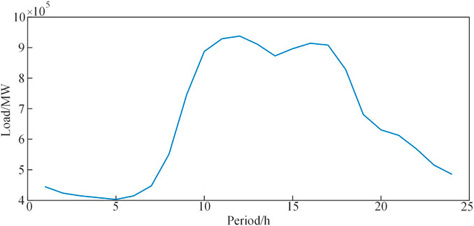
FIGURE 6. Load data of a typical day.

TABLE 2

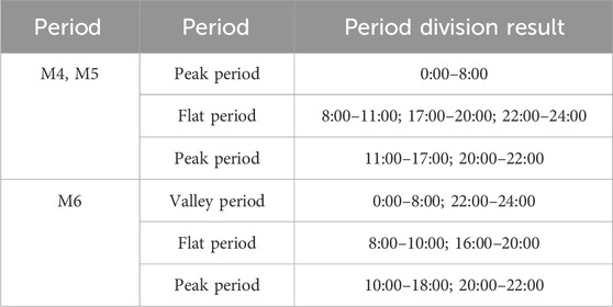
TABLE 2. Current TOU price policy of a domestic province.

Three TOU electricity tariff optimization methods M4-M6 are set up in this section, as shown in Table 3:

TABLE 3

TABLE 3. Optimization methods and effect comparison.

The load profiles after optimization by different methods are shown in Figure 7.

FIGURE 7

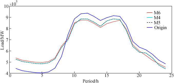
FIGURE 7. Load curve of Original and M4–M6 optimized.

The conclusions that can be drawn from Figure 7 are as follows:

1) When comparing M4, M5, and M6 with the original load curves, it is evident that M4-M6 has successfully achieved the objective of peak reduction and valley filling.

2) When compared to M4 and M5, the cost-benefit analysis of network investment in TOU electricity price optimization indicates that it will not alter its impact on the load curve.

3) In comparison to M5 and M6, the segmentation method for TOU electricity pricing periods based on the GMM clustering algorithm proposed in this study can yield further enhancements to the load curve, demonstrating the most favorable outcomes.

By optimizing the current TOU electricity pricing, users’ load curves have been enhanced, leading to peak load reduction and off-peak load increase, as well as a decrease in the investment cost of the power grid. In comparison to M4 and M5, the load curve of M6 exhibits a more pronounced peak reduction and valley filling, thereby enhancing the optimization of user load curves.

To provide additional evidence of the efficacy of the proposed approach, an analysis of the advantages for power grid companies and users is conducted, and the findings are presented in Table 4 and Table 5.

TABLE 4

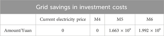
TABLE 4. Comparison of investment benefit of grid company.

TABLE 5

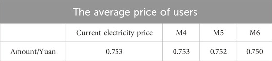
TABLE 5. Comparison of average electricity price of user.

The following conclusions can be drawn from Table 4:

1) After the implementation of the M4 TOU electricity price optimization method, the income of the power grid company has not changed compared with the original TOU electricity price strategy, the power grid company has not reduced its income due to the change of the price strategy.

2) The income of the power grid company under the M5 optimization method is significantly higher than that under the original income. This is due to the investment benefit of the power grid company is taken into account in the model, and part of the cost saved is transferred to the user, which makes the user more actively participate in peak cutting and valley filling, and effectively reduces the investment cost of the power grid.

3) The income of the power grid company under the M6 optimization method is further improved than that of M5. This is due to the period segmentation of GMM is considered in the model. Based on M5, users are more active in peak cutting and valley filling, which further reduces the investment cost of the power grid. Therefore, the M6 proposed in this paper can effectively reduce the investment cost of the power grid company and improve the income of the power grid company.

The conclusions drawn from Table 4 are as follows:

1) Following the implementation of the M4 TOU electricity price optimization method, there has been no significant change in the income of the power grid company compared to the original TOU electricity price strategy. The power grid company has not experienced a reduction in income as a result of the change in the price strategy.

2) The revenue of the power grid company is substantially greater when using the M5 optimization method compared to the original income. This phenomenon can be attributed to the incorporation of the investment benefit of the power grid company into the model, resulting in a portion of the cost savings being passed on to the user. This encourages greater user participation in peak cutting and valley filling, thereby effectively reducing the investment cost of the power grid.

3) The income of the power grid company is further enhanced under the M6 optimization method compared to that of M5. This phenomenon arises from the segmentation of periods in the Gaussian Mixture Model (GMM) as considered in the model. According to M5, users exhibit higher activity levels during peak cutting and valley filling, leading to a reduction in the investment cost of the power grid. Consequently, the M6 proposed in this study has the potential to significantly decrease the investment costs of the power grid company and enhance its revenue.

As indicated in Table 5, the unit electricity consumption for M5 users proposed in this study is 0.001 yuan less than the average price for M4 users and the original pricing strategy. Similarly, the unit electricity consumption for M6 users is 0.003 yuan lower than the average price for M4 users and the original pricing strategy. This suggests that, under the TOU electricity price period segmentation method based on the GMM, customers are experiencing cost savings on their electricity bills.

The study confirms that the TOU electricity pricing strategy proposed in this paper effectively empowers users to actively participate in peak load reduction and off-peak load utilization. This not only decreases the power grid’s investment costs but also lowers electricity expenses for users, thereby achieving a mutually beneficial outcome for both the power grid company and the users.

5 Conclusion

This paper presents an optimization method for TOU electricity pricing aimed at enhancing the user load curve, minimizing the investment cost of the power grid, and reducing the electricity expenses for consumers. The proposed method takes into account the cost savings associated with power grid investment. Firstly, the study designs the investment benefit-sharing model for the power grid and constructs a TOU price optimization model that takes into account the investment benefit of the power grid. Secondly, a method for dividing TOU electricity price periods based on the GMM clustering algorithm is proposed to obtain a reasonable division of TOU electricity price periods. Subsequently, in conjunction with the aforementioned methods and models, a comprehensive optimization strategy for TOU electricity pricing and time periods is further introduced, leading to the implementation of the TOU electricity pricing strategy design. The proposed method has been successfully verified in a provincial power system in China, demonstrating its effectiveness in designing a set of TOU electricity price strategies. This approach has the potential to create a mutually beneficial situation for power grid companies and users.

Data availability statement

The raw data supporting the conclusion of this article will be made available by the authors, without undue reservation.

Author contributions

LD: Methodology, Project administration, Writing–review and editing. LZ: Conceptualization, Writing–original draft, Writing–review and editing. LiX: Conceptualization, Data curation, Writing–review and editing. YJ: Formal Analysis, Project administration, Validation, Visualization, Writing–review and editing. YM: Conceptualization, Data curation, Writing–review and editing. LeX: Conceptualization, Methodology, Writing–review and editing.

Funding

The author(s) declare financial support was received for the research, authorship, and/or publication of this article. This work was supported by Science and Technology Project of State Grid Chongqing Electric Power Research Institute (No. 2023500016000026).

Conflict of interest

Authors LD, LiX, and YM were employed by State Grid Chongqing Electric Power Research Institute.

The remaining authors declare that the research was conducted in the absence of any commercial or financial relationships that could be construed as a potential conflict of interest.

Publisher’s note

All claims expressed in this article are solely those of the authors and do not necessarily represent those of their affiliated organizations, or those of the publisher, the editors and the reviewers. Any product that may be evaluated in this article, or claim that may be made by its manufacturer, is not guaranteed or endorsed by the publisher.

References

Chong, M. A. (2019). Research on the optimization of time-of-use electricity prices based on user electricity consumption characteristics. Beijing, China: North China Electric Power University.

Google Scholar

Cui, J., Luo, W., and Zhou, N. (2018). Research on ordered charging and discharging pricing model and strategy for electric vehicles based on multiple perspectives. Chin. J. Electr. Eng. 38 (15), 4438–4644. doi:10.13334/j.0258-8013.pcsee.171958

CrossRef Full Text | Google Scholar

Dang, X., Mao, P., and Hao, Z. (2015). A traffic clustering algorithm based on fast solving Gaussian mixture models. Comput. Eng. Appl. 51 (08), 96–101. doi:10.3778/j.issn.1002-8331.1305-0315

CrossRef Full Text | Google Scholar

Ding, ning, Wu, junji, and Zou, yun (2001a). Research on peak-valley time division and TOU price based on DSM. Proc. CSU-EPSA (23), 9–12+16.

Google Scholar

Ding, N., Wu, J., and Zou, Y. (2001b). Research on peak valley time division and time of use electricity price based on. DSM Power Syst. Autom. (23), 9–16.

Google Scholar

Domingo, C. M., Gomez San Roman, T., Sanchez-Miralles, A., Peco Gonzalez, J. P., and Candela Martinez, A. (2011). A referencenetwork model for large-scale distribution planning with automatic street map generation. IEEE Trans. Power Syst. 26 (1), 190–197. doi:10.1109/tpwrs.2010.2052077

CrossRef Full Text | Google Scholar

Dong, Q., Dong, L., and Bo, J. (2023). Optimal operation of photovoltaic-energy storage considering penetration rate of photovoltaic and division of time periods. Proc. CSU-EPSA 35 (05), 120–128. doi:10.19635/j.cnki.csu-epsa.001107

CrossRef Full Text | Google Scholar

Dong, Z., and Lin, L. (2019). Dynamic reconstruction of distribution network based on improved fuzzy C-means clustering time division. Grid Technol. 43 (07), 2299–2305. doi:10.13335/j.1000-3673.pst.2018.2461

CrossRef Full Text | Google Scholar

Gao, P., Zhao, X., Yao, F., et al. (2019). Modeling of charging loads considering the temporal and spatial distributions of electric vehicles. J. Electr. Power Sci. Technol. doi:10.19781/j.issn.1673-9140.2019.03.005

CrossRef Full Text | Google Scholar

Han, Y. (2021). Improve the policy of time of use electricity pricing with "multiple birds with one stone. China Energy News. 2021-09-06(021). doi:10.28693/n.cnki.nshca.2021.002084

CrossRef Full Text | Google Scholar

Huang, J., Yu, X., Zhao, D., Fan, Y., Chen, H., Yu, S., et al. (2023). Bi-layer optimization model of peak-valley prices and peak-valley periods considering benefits of source-grid-load [J/OL]. Electr. Power Autom. Equip. 1–13. doi:10.16081/j.epae.202312007

CrossRef Full Text | Google Scholar

Jiang, B., Li, G., Sun, Z., et al. (2021). Resident peak valley time division model based on short-term memory neural network and improved K-means clustering algorithm. Mod. Electr. Power 38 (06), 620–629. doi:10.19725/j.cnki.1007-2322.2021.0043

CrossRef Full Text | Google Scholar

Lei, X., Yang, Z., Yu, J., Zhao, J., Gao, Q., and Yu, H. (2021). Data-driven optimal power flow: a physics-informed machine learning approach. IEEE Trans. Power Syst. 36 (1), 346–354. doi:10.1109/tpwrs.2020.3001919

CrossRef Full Text | Google Scholar

Li, T. (2007). Brief introduction and research of oversea timeshare electrovalence policies. Jiangsu Electrical Engineering (01), 58–60. doi:10.19464/j.cnki.cn32-1541/tm.2007.01.019

CrossRef Full Text | Google Scholar

Li, C., Xu, Z., and Ma, Z. (2015). Time of use electricity price optimization model considering demand response of users. J. Power Syst. Automation 27 (03), 11–16.

Google Scholar

Lin, Q. (2015). Pricing and optimization of time-of-use electricity prices in smart grids. Shanghai, China: Shanghai Jiao Tong University.

Google Scholar

Liu, Q. (2006). Research on peak valley time division based on factor analysis method. Hebei: Hebei University of Technology.

Google Scholar

Min, L. I., Zhu, Y., and Hu, B. (2005). Research on peak valley time division and time of use electricity price based on power supply cost. East China Power (12), 90–91.

Google Scholar

Nedal, T. (2011). Subtractive clustering-based K-means technique for determining optimum time-of-day breakpoints. J. Comput. Civ. Eng. 25 (5), 380–387. doi:10.1061/(asce)cp.1943-5487.0000099

CrossRef Full Text | Google Scholar

Qiao, H. (2011). Research on peak valley time division method based on density clustering. Beijing: North China University of Electric Power.

Google Scholar

Ravi, N., Scaglione, A., Kadam, S., Gentz, R., Peisert, S., Lunghino, B., et al. (2022). Differentially private K-means clustering applied to meter data analysis and synthesis. IEEE Trans. Smart Grid 13 (6), 4801–4814. doi:10.1109/tsg.2022.3184252

CrossRef Full Text | Google Scholar

Ruan, W., Wang, B., Yang, L. I., and Yang, S. (2012). Research on user response behavior under peak valley time of use electricity prices. Grid Technol. 36 (07), 86–93.

Google Scholar

Sun, K. (2023). Both electricity consumption and installed power generation capacity in the whole society have achieved growth, and it is expected that the growth rate of electricity consumption demand will increase in 2023. StateGridNews. 2023-01-31(005).

Google Scholar

Wang, Q., Wang, J., and Guan, Y. (2013). Stochastic unit commitment with uncertain demand response. IEEE Trans. Power Syst. 28 (1), 562–563. doi:10.1109/tpwrs.2012.2202201

CrossRef Full Text | Google Scholar

Xing, D., Xia, L. E. I., and Jia, L. I. (2007). Using cost time curve to divide the optimal time period of time of use electricity price. Power Demand Side Manag. (04), 18–21.

Google Scholar

Yang, P., Tang, G., and Nehorai, A. (2013). A gametheoretic approach for optimal time-of-use electricity pricing. IEEE Trans. Power Syst. 28 (2), 884–892. doi:10.1109/tpwrs.2012.2207134

CrossRef Full Text | Google Scholar

Yu, R., Yang, W., and Rahardja, S. (2012). A statistical demand-price model with its application in optimal real-time price. IEEE Trans. Smart Grid 3(4), 1734–1742. doi:10.1109/tsg.2012.2217400

CrossRef Full Text | Google Scholar

Zanetti, M., Bovolo, F., and Bruzzone, L. (2015). Rayleigh-rice mixture parameter estimation via EM algorithm for change detection in multispectral images. IEEE Trans. Image Process. 24 (12), 5004–5016. doi:10.1109/tip.2015.2474710

PubMed Abstract | CrossRef Full Text | Google Scholar

Zhang, Z., and Yu, D. (2018). RBF-NN short-term load forecasting model considering comprehensive influencing factors of demand response. Chin. J. Electr. Eng. 38 (06), 1631–1899. doi:10.13334/j.0258-8013.pcsee.170835

CrossRef Full Text | Google Scholar

Zhao, C., Wang, J., Watson, J. P., and Guan, Y. (2013). Multi-stage robust unit commitment considering wind and demand response uncertainties. IEEE Trans. Power Syst. 28 (3), 2708–2717. doi:10.1109/tpwrs.2013.2244231

CrossRef Full Text | Google Scholar

Zhongfu, T., Lei, P. U., Jing, W. U., et al. (2019). Time-of-use transmission and distribution price optimization model based on differential loading rate. Syst. Eng.-Theory Pract.

Google Scholar