Frequency prediction of a post-disturbance power system using a hybrid ARIMA and DBN model

The online prediction of power system dynamic frequency helps to guide the choice of control measures quickly and accurately after a disturbance, and this then ensures the reliable and stable operations of a power system. However, the prediction performance of the traditional single model is not accurate enough, and the prediction method cannot reflect the dynamic mechanism of the power system. To address these challenges, based on the analysis of the mechanism of the dynamic operation of a power system, a dynamic frequency online prediction method using the autoregressive integrated moving average (ARIMA) model and the deep belief network (DBN) is proposed in this paper. First, according to the mechanism of the dynamic operation of a power system, the dynamic frequency can be regarded as having two stages after the disturbance occurs. In the first stage, the frequency changes monotonously in the short term, which is predicted by the ARIMA model. Furthermore, the second stage is an oscillation phase with changing amplitude, which is predicted by the DBN. The calibration process is used to combine the two predicted results. Second, the three metrics including the frequency nadir (f_nadir), the quasi-steady state frequency (f_ss), and the frequency curve obtained through the prediction are analyzed to measure the accuracy of the prediction results. Finally, to verify the accuracy of the proposed model, the IEEE 10-generator 39-bus benchmark system is used for verification.

1 Introduction

Frequency plays a crucial role in power system operations, and the frequency deviation reflects the degree of power inequality between the active power and the load capacity. In particular, the frequency remains within the safety and stability margin when a power system is operating in a steady state (Mi et al., 2021). However, after the power system is disturbed, such as the generator tripping, load outages, line switching, short circuits, or disconnection faults (Bykhovsky and Chow, 2003; Su et al., 2021), the power system may become unstable and the frequency will also change. Therefore, online frequency prediction is of great significance for assessing the stability of a power system. Furthermore, the accurate prediction of the frequency helps to schedule the power generation, which guides the control of the power system after the disturbance (Gu et al., 2018). From the viewpoint of the mechanism of a power system, when a disturbance occurs, the imbalanced power of the power system will lead to a large deviation of the frequency and instability of the power system if no control measure is activated. For example, when a serious accident occurs in a power system and the spinning reserve capacity is insufficient to make up for the power shortage, part of the load should be selectively cut to prevent the frequency from falling. This process is called under-frequency load shedding. However, frequency instability may be caused by a contingency, such as an unexpected huge demand for power without available reserve power (Wood et al., 2013). If there is no frequency prediction and no control strategy, the frequency decreases abruptly. Hence, the protection relay will be activated, and a blackout may occur in the power system. Therefore, the accurate prediction of the frequency guides the control action and ensures the safe and stable operation of power systems (Dos et al., 2015; Dahab et al., 2020).

A power system is a large-scale, highly complex, and highly nonlinear dynamic system, and it is challenging to construct the mapping function between the operation mode, the disturbance information, and the mode of the frequency response. At present, the dynamic frequency prediction methods for a power system include the time-domain simulation method, equivalent method, and machine learning method. The working principle of the time domain simulation method consists of two parts: mathematical modeling and model solving. This method is used to calculate the dynamic frequency according to the simplified model of the power system when the initial conditions are given. A set of differential-algebraic equations is constructed that represents the relationship between the various components of the power system. Then the solution of the power flow calculation is used as the initial value to solve the equations. Therefore, the frequency can be calculated.

When a power system has a large scale, the calculation amount will be large. Therefore, the time domain simulation method cannot be applied online. Furthermore, the equivalent model method can reduce the calculation amount. The equivalent model method mainly includes the average system frequency (ASF) model and the system frequency response (SFR) model. The ASF model aggregates the equations of motion of all the generator rotors in the entire network into a single-generator model. Therefore, since the independent response of the prime mover-speed control system of each generator is retained, the order of the ASF model increases when there are a large number of generators in the power system, and the calculation speed is slower. The SFR model is further simplified based on the ASF model, transforming the system into a single generator model with the centralized load. In (Anderson and Mirheydar, 1990), the frequency of the IEEE 3-generator 9-bus system after the disturbance was predicted by using the SFR model. After a 100 MW power disturbance occurred, the minimum frequency prediction error reached 0.39 Hz, and it was difficult to meet the requirements in a real-world application. Due to the simplification of the SFR model, although the calculation speed has been greatly improved, the calculation accuracy is not high. If the ASF or SFR model is adopted, a large amount of information that can be obtained will be ignored, and the model is not easy to solve.

In sharp contrast to the above methods, the machine learning methods have been used for the analysis and prediction of power system frequency dynamics (Xu et al., 2013; Yang et al., 2021). The working principle of machine learning methods is training the mapping relationship between state variables and dynamic frequencies rather than constructing complex high-order differential-algebraic equations (Xiong et al., 2021).

In (Bo et al., 2014), the v-support vector regression (v-SVR) method was used to predict the value of the frequency nadir of an IEEE 10-generator 39-bus benchmark power system after the disturbance, and the results showed that the maximum absolute error did not exceed 0.014 Hz. However, the value of the frequency can be predicted by using the v-SVR method. Several models need to be constructed when the v-SVR method is used to predict a value of the frequency. Yet, because the v-SVR models are independent of each other, the v-SVR models cannot reflect the mutual influence of factors in the change process of the frequency. In (Xu et al., 2013), the extreme learning machine was introduced into the safety margin evaluation of the power system frequency. In (Huang et al., 2018), a physical-statistical model was proposed to predict the transient stability of a power system.

Traditional types of machine learning, such as artificial neural networks, support vector machines, decision trees, and other shallow learning algorithms, are limited in terms of prediction accuracy (Aik, 2006; Shi et al., 2020). In (Hong and Wei, 2010), based on deep neural networks and a multi-layer extreme learning machine (ELM), the real-time measured data were used to predict and evaluate the frequency stability of a power system. However, there is also the problem of difficulty in determining the parameters and model structure of an ELM. In (Larsson and Rehtanz, 2002), based on SVR and artificial neural networks, the steady-state frequency of the power system for the post-disturbance period was predicted.

However, a single prediction model has the limitation of poor prediction accuracy for extreme points. According to the analysis of the power system mechanism, the frequency series is a time series containing linear and nonlinear components (Prakash et al., 2020). A hybrid model of the autoregressive integrated moving average (ARIMA) and deep belief network (DBN) models is proposed. The ARIMA model is used to predict the linear part of the frequency in this study. Furthermore, the DBN model is used to analyze and predict the residual that is predicted with the ARIMA model, which means that the nonlinear trend of the future frequency is predicted by the DBN model.

First, the linear part of the frequency is predicted by the ARIMA model. Then the residual of the predicted result is predicted with the DBN model. The DBN model is very effective in modeling the input features of the power system and the frequency, and it is effective for the nonlinear system modeling. The main contributions of this study are as follows.

1. According to the analysis of the mechanism of the dynamic operation of a power system, a dynamic frequency online prediction method using the autoregressive integrated moving average (ARIMA) model and the deep belief network (DBN) is proposed.

2. The 22 dimensional features of the power system at the moments before and after the disturbance are used as input features to predict the frequency.

3. The absolute error, maximum absolute error, mean relative error, and root mean square error of the three metrics are used to measure the accuracy of the prediction results. The three metrics include the frequency nadir (f_nadir), the quasi-steady state frequency (f_ss), and the frequency curve obtained with the prediction.

The organization of this paper is as follows. In Section 2, first, the ARIMA model is introduced. Second, the basis of the DBN model with a restricted Boltzmann machine (RBM) and a multi-layer perceptron (MLP) is presented. In Section 3, the key problems of the ARIMA-DBN model in terms of frequency prediction are illustrated. Section 4 describes how the ARIMA-DBN model is used for the frequency prediction of the IEEE 10-generator 39-bus benchmark power system. In Section 5, the conclusion is given.

2 The proposed ARIMA-DBN method

2.1 ARIMA model

Autoregressive Moving Average (ARMA) models can be represented as follows.

$\begin{array}{c}{y}_t={\theta }_0+{\varphi }_1{y}_{t-1}+{\varphi }_2{y}_{t-2}+\cdots +{\varphi }_p{y}_{t-p}\hfill \\ +{\delta }_t-{\theta }_1{\delta }_{t-1}-{\theta }_2{\delta }_{t-2}-\cdots -{\theta }_q{\delta }_{t-q}\hfill \end{array}(1)$

where y_t and δ_t are the actual value and the random error at the time period t, respectively. ϕ_i (i = 1, 2, … , p) and θ_j (j = 0, 1, 2, … , q) are parameters. $\left\{{\delta }_t\right\}$ is a sequence of independent and identically distributed random variables with a mean of zero and a constant variance of σ². p and q are the order of the autoregressive term and the moving average term, respectively (Box and Pierce, 2012). Furthermore, the number of times needed to differentiate a series in order to achieve stationarity when implementing the prediction of a time series. The ARIMA model is suitable for the modeling and prediction of the stationary series after the non-stationary series undergoes the difference operation.

The basic idea of the ARIMA model is that a certain mathematical model is used to describe the sequence that is expected to be predicted. Once the model is established, the model can be used to predict the future frequency based on the historical frequency in the time series. One key task of the ARIMA modeling is to determine the appropriate values of (p, d, q). The expression of the ARIMA model is shown below.

$\mathrm{\Phi }\left(L\right)D^d{y}_t={\theta }_0+\mathrm{\Theta }\left(L\right)u_t(2)$

where $\mathrm{\Phi }\left(L\right)$ and $\mathrm{\Theta }\left(L\right)$ are the p-order autoregressive operator and the q-order moving average operator, respectively. θ₀ is the error term. D^dy_t is the difference of the y_t by d times.

2.2 A predictor using the DBN of RBMs

2.2.1 Restricted Boltzmann machine

The Boltzmann machine is composed of the hidden layer and the visible layer. It is assumed that the visible vector is $\mathbf{v}={\left(v_1,v_2,\cdots v_m\right)}^{\text{T}}$, and the hidden vector is $\mathbf{h}={\left(h_1,h_2,\dots h_n\right)}^{\text{T}}$. In Figure 1, the unit v_i of the visible layer has the weight w_ij relative to the unit h_j of the hidden layer. Additionally, there is a two-way coupling relationship and two-way flow of data (Kuremoto et al., 2014a; Guo et al., 2015). The energy function of the RBM is defined as follows:

$\epsilon \left(v,h\mid \theta \right)=-{\displaystyle \sum _{i=1}^n}{\displaystyle \sum _{j=1}^m}{W}_{ij}{h}_i{v}_j-{\displaystyle \sum _{j=1}^m}{a}_j{v}_j-{\displaystyle \sum _{i=1}^n}{b}_i{h}_i(3)$

where W_ij represents the connection weight between the neuron i and the neuron j, a_j is the bias of the visible node j, and b_i is the bias of the hidden node i.

FIGURE 1

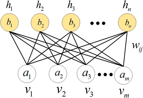
FIGURE 1. The structure of the restricted Boltzmann machine.

The training process of the RBM is to treat each training sample as a state vector in order to make the probability of the state vector’s appearance as large as possible. The joint distribution of the RBM can be obtained by using the energy function:

$p\left(v,h\mid \theta \right)=\frac{\exp \left(-\epsilon \left(v,h\mid \theta \right)\right)}{{\displaystyle \sum _{v,h}}\exp \left(-\epsilon \left(v,h\mid \theta \right)\right)}(4)$

It is assumed that there are m visible neurons and n hidden neurons, and v and h represent the state vectors of the visible layer and the hidden layer, respectively. The probability distribution can be represented as follows.

$P\left(v\mid h\right)={\displaystyle \prod _{i=1}^d}P\left(v_i\mid h\right)(5)$

$P\left(h\mid v\right)={\displaystyle \prod _{j=1}^q}P\left(h_j\mid v\right)(6)$

The RBM reaches a convergent state by learning the weights of the appropriate connections. For example, for each training sample v, first, the probability distribution of the state of the hidden layer neuron is calculated according to (6), and then h is sampled according to this probability distribution. Similarly, according to (5), v′ is generated from h, and then h′ is generated from v′. Furthermore, the update formula of the connection weight is:

$\mathrm{\Delta }W=\eta \left(\mathit{v}{\mathit{h}}^{\text{T}}-{\mathit{v}}^{\prime }{\mathit{h}}^{\prime \mathrm{T}}\right)(7)$

2.2.2 Multi-layer perceptron

Generally, the MLP includes the input layer, the hidden layer, and the output layer. The signal is input to the input layer, which is propagated to the neurons of the hidden layer. When the input signal exceeds the threshold, the neurons of the hidden layers are activated. The working principle of the output layer is similar. A logistic sigmoid function can usually be adopted as the output function of each unit, as shown in Eq. 8).

$f\left(x\right)=\frac{1}{1+\exp \left(-x/\epsilon \right)}(8)$

2.2.3 Deep belief networks

The deep belief network is composed of multiple RBMs, and the top-down generation weights determine the directional connection between the layers. Because the DBN is composed of multiple stacked RBMs, the number of visible nodes of each RBM is equal to the number of hidden layer nodes of the previous RBM (Ackley et al., 1985). The structure of a deep belief network is shown in Figure 2.

FIGURE 2

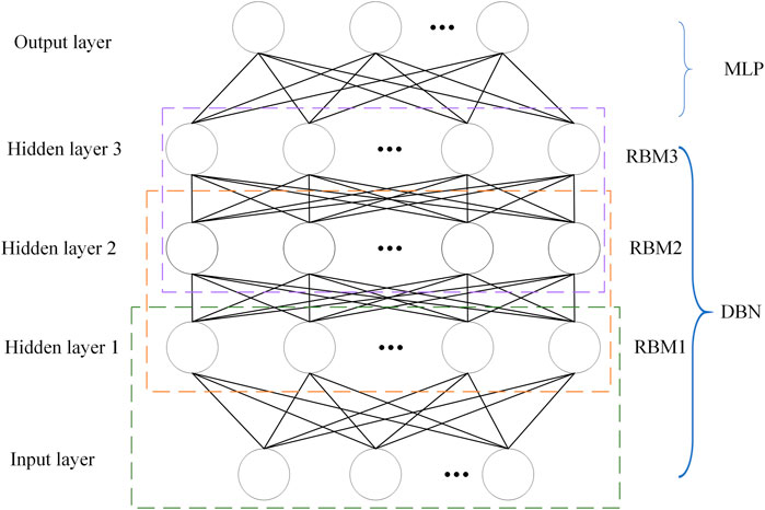
FIGURE 2. The structure of a deep belief network.

2.3 Proposed method

The linear predictor ARIMA is used for the prediction at first, and then the DBN model is used to predict the nonlinear part of the frequency. Finally, the final prediction result is the sum of the value predicted by the ARIMA model and the value predicted by the DBN model. The prediction formulas can be represented as follows.

$y\left(t\right)=L\left(t\right)+N\left(t\right)(9)$

where y(t) is the actual frequency at time t, L(t) is a linear part of y(t), and N(t) is a nonlinear part of y(t).

The ARIMA-DBN method is shown as follows:

$\epsilon \left(\mathrm{t}\right)=y\left(t\right)-\widehat{L}\left(t\right)(10)$

$\widehat{y}\left(t\right)=\widehat{L}\left(t\right)+\widehat{N}\left(t\right)(11)$

where $\widehat{L}(t)$ and $\widehat{N}(t)$ are the prediction results of the ARIMA model and the DBN model, respectively.

The framework of the ARIMA-DBN model used for frequency prediction is shown in Figure 3. First, the ARIMA model is used to predict the frequency at time t. Second, the DBN model is used to predict the error at time t, and the frequency prediction value is corrected. Finally, the calibration process is used to combine the two predicted results.

FIGURE 3

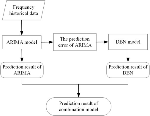
FIGURE 3. The flowchart of the proposed ARIMA-DBN method.

3 The frequency prediction of the power system after the disturbance

3.1 Description of the challenge of frequency prediction

The power system is a large-scale, highly complex, and highly nonlinear dynamic system. The frequency changes with time and the frequencies of electrical points in different geographical locations are not exactly the same. When the power system is disturbed, the dynamic changes in the frequency are caused by the comprehensive influence of all generators in the power system (Larsson, 2005; Seethalekshmi et al., 2009). Therefore, the center frequency is usually selected as the system frequency for the criterion of the actions of the frequency control. The frequency at the center inertia is as follows:

${\omega }_{COI}={\displaystyle \sum _{i=1}^n}\left(M_i{\omega }_i\right)/{\displaystyle \sum _{i=1}^n}{M}_i(12)$

where n is the number of generators. M_i and ω_COI are the inertia time constants of the i − th generator and the angular velocity of the generator rotor, respectively.

When a disturbance occurs, if no control actions are taken or the power system’s reserve capacity is not enough, the frequency is unstable. Figure 4 shows the dynamic change curve of the power system frequency at center inertia when the load increases suddenly. In the first few seconds after the disturbance occurs, due to the prime mover’s adjustment lag, the first frequency adjustment of the generator has not acted yet. The inertia of the power system determines the change speed of the frequency at center inertia. When the synchronous generator set has a frequency adjustment function, the rotating reserve of the active power is gradually put in to reduce the power imbalance. The frequency at center inertia first drops to the lowest point, then gradually rises, and finally returns to the quasi-steady state point. There are two important indicators used to measure the frequency, namely, the frequency nadir and the quasi-steady frequency.

FIGURE 4

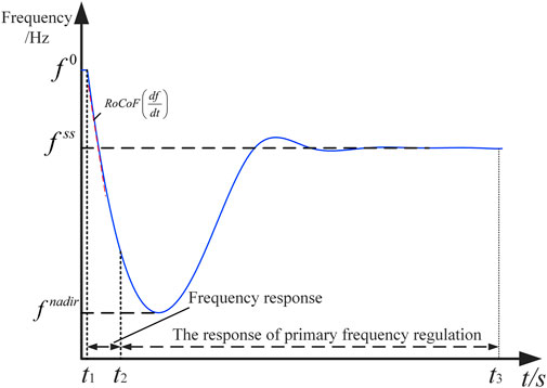
FIGURE 4. The curve of the dynamic frequency after the system is disturbed.

3.1.1 Frequency nadir f^nadir

The extreme value of the frequency is the lowest or highest point in the transient change process of the frequency at center inertia, and its magnitude is related to the system inertia, rotating reserve, and regulated power of the generator.

The frequency nadir f^nadir directly determines the acts of low-frequency load shedding when the frequency is low, and the generators are tripped when the frequency is high. This is the frequency indicator of most concern with an active power disturbance. In order to avoid generator tripping or load shedding, the value of the frequency nadir f^nadir needs to satisfy the condition of f^min ≤ f^nadir ≤ f^max, where f^min and f^max are the minimum and maximum frequencies that the power system allows for safe operations.

3.1.2 Quasi-steady frequency f^ss

f^ss is the frequency value at which the center of the inertia frequency of the system is restored to the quasi-steady state operating point after the system is disturbed. According to the value of f^nadir, it can be judged whether the power disturbance event should trigger the generator tripping or load shedding to avoid a frequency collapse.

This paper describes the use of the extreme value of the frequency at the center inertia of the power system and the quasi-steady state frequency to measure the frequency performance with disturbance events.

3.2 The selection of input features

The reasonable selection of the input feature set is the key to the ARIMA-DBN method for the frequency prediction of the power system after the disturbance. The features need to be selected with reference to the factors affecting the frequency at center inertia of the power system. Therefore, the maximum correlation and minimum redundancy algorithms are used to choose the features (Amjady and Majedi, 2007).

Therefore, in this study, the active load, reactive load, and total load amount of the system after the disturbance, as well as the reserve capacity and the total load amount of each generator at the moment and the power shortage value after the disturbance, are chosen as input features. Additionally, an extra feature is selected for the input feature set (Yurdakul et al., 2020).

From the rotor motion equation of the generator and the equation of the frequency at center inertia, the dynamic equation of the frequency of the multi-generator system can be represented as follows.

$2H\dot{\omega }=P_{\text{m}}-P_{\text{e}}-D\omega (13)$

$2H_{\mathrm{s}\mathrm{y}\mathrm{s}}{\dot{\omega }}_{\mathrm{C}\mathrm{O}\mathrm{I}}={\displaystyle \sum _{i=1}^n}{P}_{\mathrm{m}i}-{\displaystyle \sum _{i=1}^n}{P}_{\mathrm{e}i}-{\displaystyle \sum _{i=1}^n}D{\omega }_i(14)$

where H_sys represents the equivalent total inertia of the power system, ω_i, P_mi and P_ei are the frequency, mechanical power, and electromagnetic power of the i − th generator, respectively, and D represents the generator’s damping coefficient.

From Eq. 13) and Eq. 14), it can be concluded that the variables that affect the frequency at center inertia are mainly the mechanical power and the electromagnetic power of each generator (Liu et al., 2016; Zografos et al., 2018). A total of 22 dimensional features are selected in this study, as shown in Table 1. Given the input features mentioned above and the prediction error of the ARIMA model, the established mapping network can reflect the influence of the 22 features on the frequency and include the influence of the system control parameters on the current system frequency.

TABLE 1

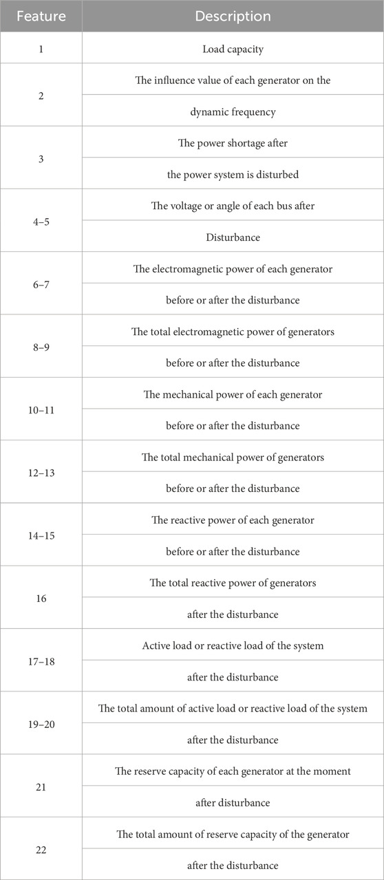
TABLE 1. Input features of frequency prediction.

3.3 Modeling process

From the perspective of the power system mechanism, the dynamic frequency can be regarded as having two stages after the power system is disturbed. In the first stage, the frequency changes monotonously in the short term. The second stage is an oscillation phase with changing amplitude. In the first stage, the frequency changes approximately linearly. Furthermore, the first stage reflects the characteristics of the frequency, which contains more information about the whole power system. Specifically, the type of disturbance and the capacity amount of the disturbance are contained in the frequency characteristics in the first stage. The dynamic part of the frequency of the power system is regarded as nonlinear in the second stage.

The basic idea of the hybrid method is as follows. First, the ARIMA model is used to predict the frequency. Then the DBN is used to obtain a more accurate result of the predicted frequency. The linear prediction result is obtained with the ARIMA model, and then the residual value is obtained by determining the difference between the original frequency and the linear prediction result. The residual values represent the nonlinear characteristics of frequency. The error sequence can also be regarded as a random time sequence, and its error prediction model can also be established. Then the DBN model is used to analyze and predict the residual values (Hinton, 2012; Kuremoto et al., 2014b). Finally, the results of the linear prediction and the nonlinear prediction are summed to obtain the prediction frequency. The proposed ARIMA-DBN model can effectively solve the limitations of a single model’s low prediction accuracy.

The specific modeling and the prediction process of the ARIMA-DBN model used for frequency prediction are shown in Figure 5. The realization of the hybrid prediction method based on the ARIMA-DBN model is as follows. First, the ARIMA model is used to predict the frequency at time t. Second, the DBN model is used to predict the error at time t, and the frequency prediction value is corrected. The dotted line in Figure 5 is the modeling process of the error prediction.

FIGURE 5

FIGURE 5. Hybrid ARIMA and DBN model for frequency prediction.

After the modeling process is completed, an error prediction model is formed, as shown by the solid rectangular frame, which is used to predict the prediction error and correct the prediction frequency. By analyzing a large quantity of historical data, a reasonable frequency prediction model that reflects the changing trend of the historical data can be established.

4 Case study

The IEEE 10-generator 39-bus benchmark system is adopted to evaluate the performance of the proposed ARIMA-DBN model. This benchmark system comprises 10 generators, 39 buses, 19 loads, 12 transformers, and 34 transmission lines, as shown in Figure 6. The rated frequency is 60 Hz. The base power and the voltage are 100 MVA and 345 kV, respectively. The generator at bus 39 represents the aggregation of a large system.

FIGURE 6

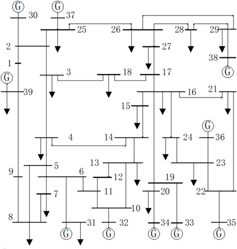
FIGURE 6. The topology of the IEEE 10-generator 39-bus system.

4.1 Dataset generation

Since various disturbances such as generator tripping or a load increase or decrease may occur to different degrees, multiple emergency scenarios are generated for analysis. Power System Simulator/Engineering (PSS/E) can be used to simulate numerous contingencies in batch mode, which is useful in transient analysis. Consequently, the required numerical simulations are run on the IEEE 10-generator 39-bus benchmark system by using PSS/E. Based on the IEEE 10-generator 39-bus benchmark system, the transient simulation after the sudden load increase, the sudden load decrease, and the generator tripping disturbance is carried out.

The setting of the simulation conditions is mainly divided into two parts, namely, the setting of the operation mode and the setting of the disturbance information. The setting of the operation mode mainly involves consideration of the load capacity, load model, rotating reserve, and inertia time constant. All the loads (both active and reactive loads) are set to 50%, 50.25%, 50.5%,…, 110% of the rated load capacity, respectively. The rotating reserves of the power system are set to 0%, 0.5%, 1.0%,…, 4.0% of the basic value, respectively. For the simulation of different working conditions of the power system, the inertia time constant is set to 0.2 times, 0.4 times, 0.6 times, … , 2.0 times the basic value, respectively. The detailed configurations are listed in Table 2.

TABLE 2

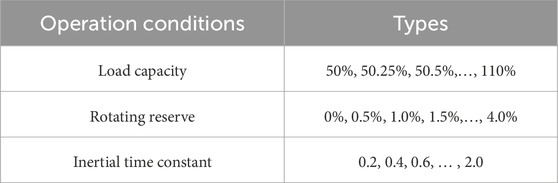
TABLE 2. Operation mode setting.

For the disturbance cases, the fault types are a short-circuited fault, line shedding fault, bus short-circuit fault, and generator tripping disturbance. The disturbances of the load increase or load shedding are set to 5%, 10%, 15%,…, 100% of the rated load capacity. The generator tripping is determined by the generator capacity of the simulation system.

According to the above operation mode settings and disturbance information settings, different combinations of operation modes and disturbances can be selected arbitrarily to form different scenarios of the transient simulation. A large number of data samples for frequency prediction can be obtained after the transient simulation. First of all, the rotating reserve, inertia time constant, and active power in the power system can be continuously changed for the same load capacity, and different load models for the transient simulation can be set. Thus, several steady-state operation modes before disturbance can be obtained. In a certain operating mode, different fault types and fault locations are set, and then the data samples of different frequency response modes for the above corresponding conditions can be obtained through transient simulation.

Each load mode of the IEEE 10-generator 39-bus benchmark system has 12 groups of switching load disturbances, and each line has two cutoff line disturbances after a short circuit. Therefore, for one scenario of steady-state operation, 294 different disturbances and frequency response curves can be generated. For the simulation of generator tripping, the time of a single simulation is 60 s. The step length is 0.01 s. The frequency needs to be obtained with the weighted average of the frequency of each generator according to the inertia time constant. Figures 7, 8 show the system frequency at the center inertia response results. The frequency at center inertia after a 500-MW generator is tripped shown in Figure 7. The frequency at center inertia after 90-MW load shedding is shown in Figure 8.

FIGURE 7

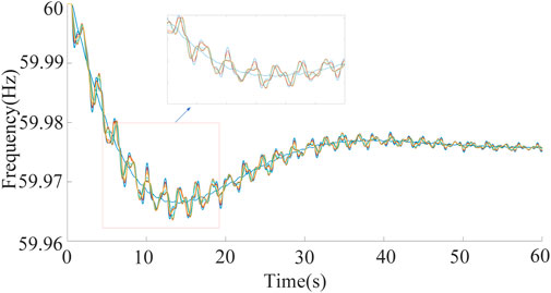
FIGURE 7. The frequency at center inertia after the generator tripping.

FIGURE 8

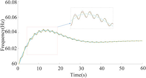
FIGURE 8. The frequency at center inertia after the load shedding.

4.2 Evaluation indicators

To assess the prediction accuracy of different models, the absolute error (AE), maximum absolute error (MAE), mean relative error (MRE), and root mean square error (RMSE) are used to evaluate the results. The MRE is the ratio of the error of the true value, which means that the smaller the value of the MRE is, the higher the accuracy of the prediction result is. The root mean square error can reflect the degree of dispersion of the error, that is, the stationarity of the prediction. When there is a very small number of values that differ greatly from the real values, the RMSE indicator is greatly affected. The formulas of the above four indicators are as follows.

$\mathrm{A}\mathrm{E}=f\left(x_i\right)-y_i(15)$

$\mathrm{M}\mathrm{A}\mathrm{E}=\max \left(\mathrm{a}\mathrm{b}\mathrm{s}\left|f\left(x_i\right)-y_i\right|\right)(16)$

$MRE=\frac{1}{n}{\displaystyle \sum _{i=1}^n}\frac{\left|X_i-Y_i\right|}{Y_i}(17)$

$RMSE=\sqrt{\frac{1}{n}{\displaystyle \sum _{i=1}^n}{\left(X_i-Y_i\right)}^2}(18)$

4.3 Analysis of prediction result

4.3.1 Frequency nadir

Three methods including the ARIMA-DBN model, support vector regression (SVR), and the back-propagation neural network (BPNN) model are adopted for frequency prediction. The frequency nadir is extracted, and the error calculation is performed. The result is shown in Table 3 and Figure 9.

TABLE 3

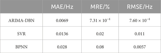
TABLE 3. Comparison of the accuracy of different methods for predicting f_nadir.

FIGURE 9

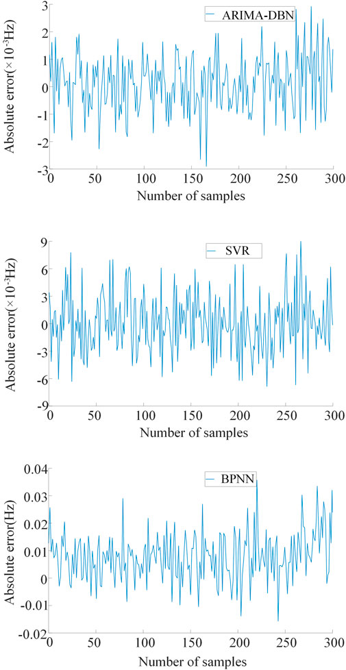
FIGURE 9. Absolute error comparison of the f_nadir.

It can be concluded from Table 3 and Figure 9 that the error of the ARIMA-DBN used to predict the minimum value of frequency is very small. Table 3 shows that the maximum absolute error of the lowest value predicted by the ARIMA-DBN model is 0.0069 Hz, and the mean relative error is 7.31 × 10⁻⁴%.

4.3.2 The quasi-steady state frequency

Three methods including the ARIMA-DBN model, SVR model, and the BPNN model are used for frequency prediction of the power system after the disturbance. The quasi-steady state frequency is extracted, and the error is calculated. The result is indicated in Table 4 and Figure 10.

TABLE 4

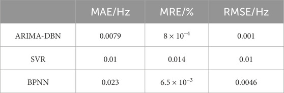
TABLE 4. Comparison of the accuracy of different methods for predicting f_ss.

FIGURE 10

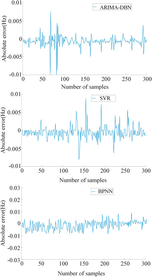
FIGURE 10. Absolute error comparison of the f_ss.

It can be concluded from Table 4 and Figure 10 that the error of the ARIMA-DBN used to predict the steady-state value of frequency is very small, and the accuracy of the BPNN in predicting the steady-state value of frequency is generally better than that of SVR. The maximum absolute error of the steady-state value predicted by the ARIMA-DBN model is 0.0079 Hz, and the mean relative error is 8 × 10⁻⁴%.

4.3.3 The dynamic characteristics of the frequency

The prediction result of the frequency curve of the 37th sample is shown in Figure 11.

FIGURE 11

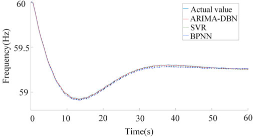
FIGURE 11. Frequency curve of the 37th test sample.

It can be seen from Figure 11 that the maximum absolute error of SVR when predicting the frequency curve is slightly smaller than that of the ARIMA-DBN model, but the root mean square error of the ARIMA-DBN model when predicting the frequency curve is much lower than that of SVR and the BPNN. As can be seen from Figure 11, compared to the other two methods, the ARIMA-DBN prediction curve has a high degree of overlap with the simulation curve, and the SVR prediction curve has a large prediction error at the steady-state value of the frequency. Taking this sample as an example, the frequency is 58.91 Hz, which is lower than the frequency setting value of 59.5 Hz. For this kind of disturbance, the power system is assessed to be unstable. Therefore, the automatic load shedding control is activated.

The load to be removed is calculated according to the predicted minimum frequency value and the corresponding load is removed so that the actual frequency of the system is not lower than the set value. The results show that the proposed method can predict the frequency curve value within 60 s after the disturbance, which is quicker and more accurate than other single machine learning methods.

5 Conclusion

The frequency of the power system after the disturbance is predicted using a hybrid model of the autoregressive integrated moving average model and a deep belief network. The 22 dimensional features of the power system at the moments before and after the disturbance are used as input features to predict the frequency, and the IEEE 10-generator 39-bus system is adopted for verification. Compared with traditional machine learning models, such as the SVR model and BPNN, the frequency prediction result of the hybrid ARIMA-DBN model is more accurate according to the comparison of the absolute error, the maximum absolute error, the mean relative error, and the root mean square error of three metrics, including the frequency nadir, the quasi-steady state frequency, and the dynamic characteristics of frequency. In the future research, according to the result of the predicted frequency, study the emergency control strategy to ensure the frequency stability further.

Data availability statement

The raw data supporting the conclusion of this article will be made available by the authors, without undue reservation.

Author contributions

HW: Investigation, Methodology, Software, Writing–original draft, Writing–review and editing. ZL: Supervision, Validation, Writing–review and editing. JP: Supervision, Writing–review and editing. WC: Supervision, Writing–review and editing.

Funding

The author(s) declare that no financial support was received for the research, authorship, and/or publication of this article.

Conflict of interest

The authors declare that the research was conducted in the absence of any commercial or financial relationships that could be construed as a potential conflict of interest.

Publisher’s note

All claims expressed in this article are solely those of the authors and do not necessarily represent those of their affiliated organizations, or those of the publisher, the editors and the reviewers. Any product that may be evaluated in this article, or claim that may be made by its manufacturer, is not guaranteed or endorsed by the publisher.

References

Ackley, D. H., Hinton, G. E., and Sejnowski, T. J. (1985). A learning algorithm for Boltzmann machines. Cognitive Sci. 9, 147–169. doi:10.1016/s0364-0213(85)80012-4

CrossRef Full Text | Google Scholar

Aik, D. L. H. (2006). A general-order system frequency response model incorporating load shedding: analytic modeling and applications. IEEE Trans. Power Syst. 21 (2), 709–717. doi:10.1109/tpwrs.2006.873123

CrossRef Full Text | Google Scholar

Amjady, N., and Majedi, S. F. (2007). Transient stability prediction by a hybrid intelligent system. IEEE Trans. Power Syst. 22 (3), 1275–1283. doi:10.1109/tpwrs.2007.901667

CrossRef Full Text | Google Scholar

Anderson, P. M., and Mirheydar, M. (1990). A low-order system frequency response model. IEEE Trans. Power Syst. 5 (3), 720–729. doi:10.1109/59.65898

CrossRef Full Text | Google Scholar

Bo, Q., Wang, X., and Liu, K. (2014). “Minimum frequency prediction of power system after disturbance based on the v-support vector regression,” in 2014 International Conference on Power System Technology, Chengdu, China, October 2014.

Google Scholar

Box, G. E., and Pierce, D. A. (2012). Distribution of residual autocorrelations in autoregressive-integrated moving average time series models. J. Am. Stat. Assoc. 65, 1509–1526. doi:10.1080/01621459.1970.10481180

CrossRef Full Text | Google Scholar

Bykhovsky, A., and Chow, J. H. (2003). Power system disturbance identification from recorded dynamic data at the Northfield substation. Int. J. Elec. Power 25 (10), 787–795. doi:10.1016/s0142-0615(03)00045-0

CrossRef Full Text | Google Scholar

Dahab, Y. A., Abubakr, H., and Mohamed, T. H. (2020). Adaptive load frequency control of power systems using electro-search optimization supported by the balloon effect. IEEE Access 8, 7408–7422. doi:10.1109/access.2020.2964104

CrossRef Full Text | Google Scholar

Dos, E., Neto, J. J., Marchesan, G., and Cardoso, G. (2015). Power system frequency estimation using morphological prediction of Clarke components. Electr. Pow. Syst. Res. 122, 208–217. doi:10.1016/j.epsr.2015.01.012

CrossRef Full Text | Google Scholar

Gu, H., Yan, R., and Saha, T. K. (2018). Minimum synchronous inertia requirement of renewable power systems. IEEE Trans. Power Syst. 33 (2), 1533–1543. doi:10.1109/tpwrs.2017.2720621

CrossRef Full Text | Google Scholar

Guo, J., Li, Z., and Pecht, M. (2015). A Bayesian approach for li-ion battery capacity fade modeling and cycles to failure prognostics. J. Power Sources 281, 173–184. doi:10.1016/j.jpowsour.2015.01.164

CrossRef Full Text | Google Scholar

Hinton, G. E. (2012). “A practical guide to training restricted Boltzmann machines,” in Neural networks: tricks of the trade, 599–619.

CrossRef Full Text | Google Scholar

Hong, Y. Y., and Wei, S. F. (2010). Multiobjective underfrequency load shedding in an autonomous system using hierarchical genetic algorithms. IEEE Trans. Power Deliv. 25 (3), 1355–1362. doi:10.1109/tpwrd.2010.2046679

CrossRef Full Text | Google Scholar

Huang, D., Yang, X., Chen, S., and Meng, T. (2018). Wide-area measurement systemised model-free approach of post-fault rotor angle trajectory prediction for on-line transient instability detection. IET Gener. Transm. Dis. 12 (10), 2425–2435. doi:10.1049/iet-gtd.2017.1523

CrossRef Full Text | Google Scholar

Kuremoto, T., Kimura, S., Kobayashi, K., and Obayashi, M. (2014a). Time series forecasting using a deep belief network with restricted Boltzmann machines. Neurocomputing 137, 47–56. doi:10.1016/j.neucom.2013.03.047

CrossRef Full Text | Google Scholar

Kuremoto, T., Obayashi, M., Kobayashi, K., Hirata, T., and Mabu, S. (2014b). “Forecast chaotic time series data by DBNs,” in Ieee T. Power syst, 1130–1135.

CrossRef Full Text | Google Scholar

Larsson, M. (2005). “An adaptive predictive approach to emergency frequency control in electric power systems,” in Proceedings of the 44th IEEE Conference on Decision and Control, Seville, Spain, December 2005, 4434–4439.

Google Scholar

Larsson, M., and Rehtanz, C. (2002). “Predictive frequency stability control based on wide-area phasor measurements,” in IEEE Power Engineering Society Summer Meeting, Chicago, IL USA, July 2002.

Google Scholar

Liu, S., Li, G., and Zhou, M. (2016). Power system transient stability analysis with integration of dfigs based on center of inertia. CSEE J. Power Energy 2 (2), 20–29. doi:10.17775/cseejpes.2016.00018

CrossRef Full Text | Google Scholar

Mi, Y., Xu, Y., Lang, Z., Yang, X., Ge, X., Fu, Y., et al. (2021). The frequency-voltage stability control for isolated wind-diesel hybrid power system. Electr. Pow. Syst. Res. 192 (1), 106984. doi:10.1016/j.epsr.2020.106984

CrossRef Full Text | Google Scholar

Prakash, T., Mohanty, S. R., and Singh, V. P. (2020). PMU-assisted zone-3 protection scheme for pv integrated power systems immune to interharmonics. IEEE Syst. J. 14 (3), 3267–3276. doi:10.1109/jsyst.2020.2964742

CrossRef Full Text | Google Scholar

Seethalekshmi, K., Singh, S., and Srivastava, S. (2009). “WAMS assisted frequency and voltage stability based adaptive load shedding scheme,” in 2009 IEEE Power and Energy Society General Meeting, Alberta, Canada, October 2009, 1–8.

CrossRef Full Text | Google Scholar

Shi, Z., Yao, W., Zeng, L., Wen, J., Fang, J., Ai, X., et al. (2020). Convolutional neural network-based power system transient stability assessment and instability mode prediction. Appl. Energy 263, 114586. doi:10.1016/j.apenergy.2020.114586

CrossRef Full Text | Google Scholar

Su, Y., Li, H., Cui, Y., You, S., Ma, Y., Wang, J., et al. (2021). An adaptive PV frequency control strategy based on real-time inertia estimation. IEEE Trans. Smart Grid 12 (3), 2355–2364. doi:10.1109/tsg.2020.3045626

CrossRef Full Text | Google Scholar

Wood, A. J., Wollenberg, B. F., and Sheblé, G. B. (2013). Power generation, operation, and control. New Jersey, United States: John Wiley and Sons.

Google Scholar

Xiong, L., Liu, X., Zhang, D., and Liu, Y. (2021). Rapid power compensation based frequency response strategy for low inertia power systems. IEEE J. Em. Sel. Top. P. 9 (4), 4500–4513. doi:10.1109/jestpe.2020.3032063

CrossRef Full Text | Google Scholar

Xu, Y., Dai, Y., Dong, Z. Y., Zhang, R., and Meng, K. (2013). Extreme learning machine-based predictor for real-time frequency stability assessment of electric power systems. Neural comput. Appl. 22 (3), 501–508. doi:10.1007/s00521-011-0803-3

CrossRef Full Text | Google Scholar

Yang, H., Liu, X., Zhang, D., Chen, T., Li, C., and Huang, W. (2021). Machine learning for power system protection and control. Electr. J. 34 (1), 106881. doi:10.1016/j.tej.2020.106881

CrossRef Full Text | Google Scholar

Yurdakul, O., Eser, F., Sivrikaya, F., and Albayrak, S. (2020). Very short-term power system frequency forecasting. IEEE Access 8 (1), 141234–141245. doi:10.1109/access.2020.3013165

CrossRef Full Text | Google Scholar

Zografos, D., Ghandhari, M., and Eriksson, R. (2018). Power system inertia estimation: utilization of frequency and voltage response after a disturbance. Electr. Pow. Syst. Res. 161, 52–60. doi:10.1016/j.epsr.2018.04.008

CrossRef Full Text | Google Scholar