 Kezheng Jiang
 Chang Ye1
 Yang Chen
 Pan Hu
- 1State Grid Hubei Electric Power Research Institute, Wuhan, China
- 2Department of Information Science and Engineering, Wuhan University of Science and Technology, Wuhan, China
The small-signal stability of high voltage direct current (HVDC)-connected wind farms (WFs) is a challenging issue in modern power systems. The relative stability, i.e., the stability margin, of such a typical multiple-input multiple-output (MIMO) system is quite difficult to be quantified. This paper evaluates the relative stability of HVDC-connected WFs using a new stability index based on the ν-gap metric. We first develop a MIMO model represented by a transfer function matrix of the HVDC-connected WFs. Then, a new stability index, i.e., the robust stability margin, based on the ν-gap metric is proposed to quantify the relative stability of such a MIMO system. Finally, we propose a method to compute the stable region of control parameters based on the corresponding stability criterion of ν-gap metric. Case studies are given to demonstrate the effectiveness of the proposed method.
1 Introduction
Nowadays, line-commutated converter based HVDC system is widely used for long-distance transmission of renewable energies, especially in China. In recent years, several subsynchronous oscillations have occurred in the HVDC systems connected with renewable energy generations, e.g., the oscillation phenomena in the Hami grid of China’s Xinjiang Province, which seriously threaten the stability of modern power systems.
The small-signal stability of HVDC-connected WFs has attracted a lot of attention from researchers. Eigenvalue analysis method is one of the commonly used approach for stability analysis (Zhou et al., 2011; Yogarathinam et al., 2017; Ángel Cardiel-Álvarez et al., 2017). Based on the state-space model of the overall system, the eigenvalues, participation factors and sensitivity of control parameters are calculated (Yogarathinam et al., 2017; Ángel Cardiel-Álvarez et al., 2017; Shen et al., 2021). Some insights of the oscillations can be found from the analysis results. A state-space model of Gravelines generator and IFA2000 HVDC system is established (Kovacevic et al., 2019). The results show that damping of the 6.3 Hz mode can be improved while the damping of 12 Hz mode can be deteriorated by increasing the proportional parameters of DC current controller and PLL.
Impedance analysis is also a widely used method to analyze the stability of the HVDC-connected WFs. The impedance models of HVDC-connected WFs are developed in (Liu and Sun, 2013a; b), and the stability of the systems are analyzed based on the Nyquist criterion (Sun, 2011; Liu et al., 2014; Wang et al., 2022b). Researchers compared the influence of different control parameters on the impedance characteristics of the system in (Wang et al., 2022a; Wang et al., 2020). Considering the effect of DC control system, an impedance modeling method of control system based on transfer function is proposed in (Su et al., 2023). The results show that the constant current control of the rectifier has resonance risk near a specific frequency.
However, the above methods mainly focus on determining whether the system is stable or not. It is difficult for them to assess the relative stability, i.e., the stability margin, of the system and measure how far the system is away from instability. A better relative stability performance indicates that the system can tolerate a larger range of parameter variation.
On the other hand, gain margin and phase margin are measurements of the relative stability of a single-input single-output (SISO) system in classical control theories. Researchers use gain and phase margin to analyze and design the control systems in the context of robust stabilization (Bayhan and Soylemez, 2007). Based on the impedance model of WFs, phase and gain margin can be calculated from Nyquist curve (Rohit et al., 2021). However, since phase and gain margin are calculated by the open-loop transfer function of a unit feedback system, they are only available for SISO systems. It is difficult to compute the phase and gain margin of the HVDC-connected WFs, which is a typical MIMO system with multiple devices. To address this issue, we come up with the idea of applying the ν-gap metric to measure the stability margin of the system. The ν-gap metric theory is commonly used to investigate the robustness of stability in feedback interconnected systems (Vinnicombe, 2001; Jiang et al., 2021), especially for MIMO systems.
In this paper, we analyze the relative stability of a HVDC system connected with WFs utilizing the ν-gap metric. The contributions of this paper are as follows:1) We build a small-signal model of a HVDC system connected with WFs represented by transfer function matrix, in which the internal current vector and the active/reactive power are the input and output signals. 2) A new stability index, i.e., the robust stability margin, based on the ν-gap metric is proposed to quantify the relative stability of such a MIMO system. Compared with phase and gain margin, the proposed robust stability margin can be calculated directly on the basis of the proposed MIMO model of the system. 3) Based on the sufficient and necessary stability criterion of the ν-gap metric, we propose a method to compute the stable region of the control and operation parameters of the system.
The rest of this paper is organized as follows. Chapter 2 presents the original small-signal model of HVDC- connected WFs and the basic definitions of the ν-gap metric. Chapter 3 develops a standardized feedback model of HVDC- connected WFs applicable to he ν-gap metric. Furthermore, the robust stability margin and the method to compute the stable region of control and operation parameters is presented in Chapter 4. Simulation results are proposed in Chapter 5, and conclusions are drawn in Chapter 6.
2 Related work
In this section, we show the related work of this paper. Firstly, we present the original small-signal model proposed in (Yuan et al., 2017; Lu et al., 2020) based on the typical control scheme of a HVDC system and WFs. Then, the basic definitions and the stability criterion based on the ν-gap metric are introduced.
2.1 Original small-signal model in DVC timescale
Figure 1 shows a HVDC system connected with two WFs. This paper mainly focuses on the power sending terminal containing the rectifier of the HVDC and the GSCs of the WFs. In such a system, P and Q represent active power and reactive power.
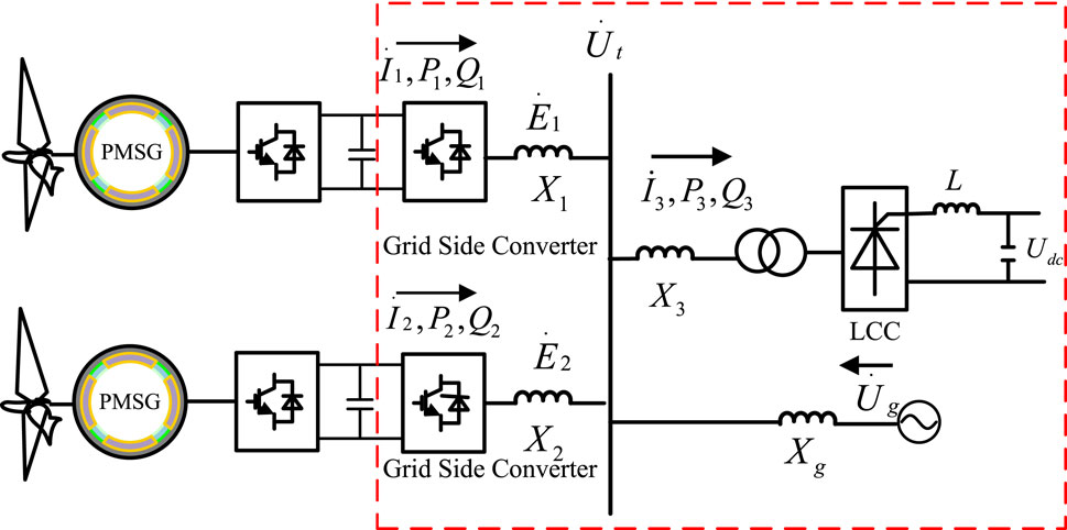
Figure 1. Topology diagram of a rectifier connected with two WFs.
According to (Lu et al., 2020), Figure 2A shows the typical control strategy of the rectifier of a HVDC system. DC current control (DCC) is applied to control the DC current and generate an appropriate order triggering angle αord for the thyristors. At the same time, a phase-locked loop (PLL) is used to capture the phase of the AC terminal voltage. The value of αord is the sum of actual triggering angle and PLL’s angle.
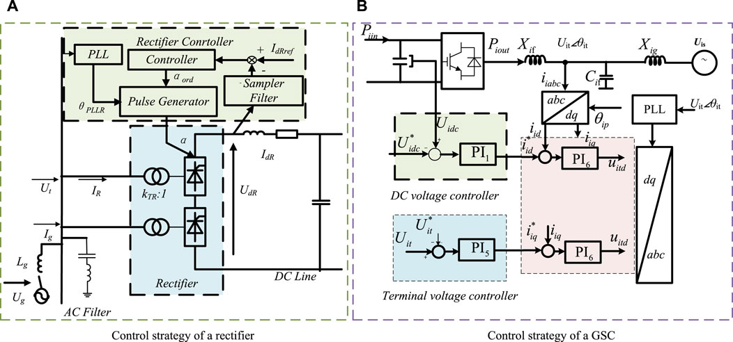
Figure 2. Control strategies of the rectifier of HVDC and GSCs of the WFs. (A) Control strategy of a rectifier. (B) Control strategy of a GSC.
Figure 2B depicts the typical control strategy of a GSC, including DC voltage control (DVC), reactive power control (RPC), inner current control (ICC) and PLL. The active branch controls the DC voltage and the AC current in d-axis. The reactive branch controls the reactive power and the AC current in q-axis. Similar with the rectifier of HVDC, all the above control are controlled on the PLL synchronization reference frame.
Utilizing the above control strategies, the small-signal models of a rectifier and a GSC in DVC timescale (about 10 Hz) are proposed in (Yuan et al., 2017; Lu et al., 2020), respectively. Figure 3A depicts the original small-signal model of a rectifier. Figure 3B depicts the original small-signal model of a GSC. In these models, the active and reactive power are the input signals and the phase and magnitude of the internal voltage or current are the output signals. They describe the dynamic characteristics of the rectifier and the GSC with clear mechanism understanding based on the motion equation concept.
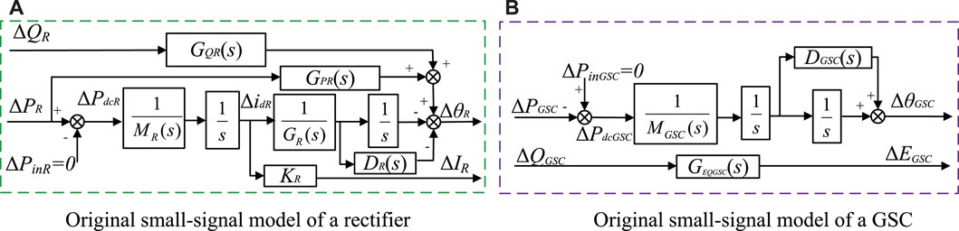
Figure 3. Original small-signal model of the rectifier of HVDC and the GSC of the WFs. (A) Original small-signal model of a rectifier. (B) Original small-signal model of a GSC.
2.2 Basic theory of ν-gap metric
The basic theory of ν-gap metric is proposed (Zhou, 2010) to analyze the robust stability of a feedback system. Consider a nominal feedback system depicted in Figure 4A. P(s) is the forward channel and C(s) is the feedback channel. The robust stability margin to quantify the relative stability is denoted as b [P(s), C(s)]. If the system is stable, b [P(s), C(s)] is in the interval (0,1]. If the system is unstable, b [P(s), C(s)] = 0.
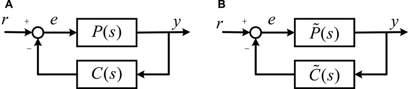
Figure 4. Standard model block diagram. The left image is (A), and the right image is (B).
For the corresponding feedback system with uncertainties as shown Figure 4B.
the uncertain system is stable. Otherwise, the uncertain system is unstable.
It is worth noticing that the system can be a SISO system or a MIMO system. Furthermore, the stability criterion is a necessary and sufficient condition without any conservatism.
3 Modeling of a HVDC system connected with WFs
In this section, based on the original small-signal model in Figure 5, we build a MIMO system model for the relative stability analysis. First, we present the forward channel of the MIMO system model by transfer function matrix. Then, we establish the feedback channel reflecting the power flow in AC network by transfer function matrix.
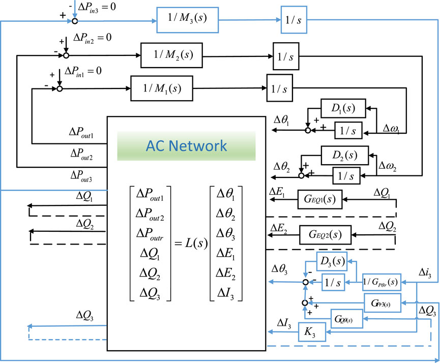
Figure 5. Small signal model.
3.1 Modeling of the forward channel
In this subsection, we build the forward channel of the MIMO system model reflecting the dynamic characteristics of the rectifier and GSCs.
On the basis of the rectifier model shown in Figure 3A the GSC model shown in Figure 3B, we establish the small-signal model of the HVDC system connected with two GSCs in Figure 5. In this model, ΔPin represents the active power input of the DC inductance and DC capacitors of each device. ΔPout and ΔQout represent the active and reactive power output of the DC inductance and DC capacitors of each device. Δθ and ΔE represent the phase and magnitude of the internal voltage. Denote Δθ and ΔI as phase and magnitude of the internal current of the rectifier. Transfer functions M(s) and D(s) represent the equivalent inertia and damping, respectively. GEQ(s) is the transfer function related to the reactive power control. GPr3(s) is a partial transfer function between ΔPout and Δθ of the rectifier. Denote Δi3 as AC current of the rectifier. GPθr(s) is a partial transfer function between Δi3 and Δθ of the rectifier. K3 is a proportionality transfer function between DC current dynamics and ΔI of the rectifier. J6 × 6 is an admittance matrix of the power flow in AC network. Specific expressions of the matrix and the transfer functions are provided in Supplementary Appendix SA according to (Yuan et al., 2017; Lu et al., 2020).
For the GSCs in the model, the transfer function between Δθ of the internal voltage and ΔPout of GSC 1 can be expressed as
The transfer function between Δθ of the internal voltage and ΔPout of GSC 2 can be described as
For the rectifier in the model, denote the transfer function GPθ3(s) between Δθ of the internal current and ΔPout of the rectifier as
The transfer function between ΔI and ΔPout of the rectifier can be described as
Specific expressions of GEQ1, GEQ2, GQθ are given in (Lu et al., 2020). For compact expressions, denote
Then, the forward channel of the MIMO system can be described as
where
3.2 Modeling of the feedback channel
Next, let’s establish the model of the AC network, i.e., the feedback channel of the MIMO system.
As seen from Figure 5, the feedback channel reflects the power flow of the AC network. Since the input signals of the AC network contains the phase and magnitude of both the internal voltage and internal current, we need to derive the Jacobian matrix of the mixed system.
First, we calculate the branch circuit across each device. For the system shown in Figure 1, the current of each branch can be expressed as
According to the Kirchhoff’s Current Law, the current flowing through the rectifier is
Based on (8) and (9), the AC voltage on the bus can be calculated as
By substituting (10) into (8), the current of the two GSCs can be obtained as
where Y11, Y12, G13, Y1g, Y21, Y22, G23, Y2g are the elements of the admittance matric as shown in Supplementary Appendix SA. The internal voltage of the rectifier can be described as
By substituting (10) into (12), we have
where the elements of the admittance matric Y31, Y32, G33, Y3g are as shown in Supplementary Appendix SA.
Then, the apparent power of the GSCs and the rectifier can be calculated as.
where
According to (11) and (13) into (14), the active power and reactive power of each branch can be expressed as.
Linearizing (17) at the steady-state operating point yields.
In (23), KPθ11 ∼ KPθ33, KPE11 ∼ KPI33, KQθ11 ∼ KQθ33, KQE33 ∼ KQI33 are shown in Supplementary Appendix SA. Denote
Then, the feedback channel (23) can be written as
where
Then, the entire model of the system represented by transfer function matrix can be illustrated by Figure 6. In this model, ΔS represent the set of the input signals and ΔV represent the set of the output signals. H(s) and L(s) represent the forward and feedback channels, respectively.
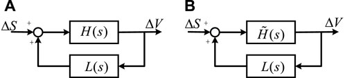
Figure 6. Standard feedback model of the HVDC system connected with WFs. The left image is (A), and the right image is (B).
4 Relative stability analysis and stable region computation
To analysis the relative stability of the system, we calculate the robust stability margin of the system first. Then, the methodology of assessing the stable region of parameters is illustrated.
4.1 Robust stability margin
In this subsection, we propose a new index, i.e., the robust stability margin based on the ν-gap metric to evaluate the relative stability of the MIMO system.
For a standard feedback system as depicted in Figure 6A, if the system is stable, the robust stability margin bH,L of Figure 6A are defined as
where
The proposed robust stability margin can be used to assess the relative stability of the system. If the system is stable, bH,L is in the interval (0,1]. The larger bH,L is, the more stable the system is. When the system is unstable, bH,L equals to 0. Compared with other stability margin, i.e., phase margin and amplitude margin, the proposed robust stability margin can be directly computed in a MIMO systems.
4.2 Stable region of parameters
In this subsection, we will clarify the methodology of calculating the stable region of parameters. From the point view of control, the stable region for the control systems can be obtained by calculating the ranges of uncertain parameters preserving the system stability. In this paper, we mainly focus on assessing the stable region of the control parameters in DVC, DCC and PLL of the GSCs and the rectifier. The structure and the power flow of the network are considered to be fixed. It means that the uncertainties exist only in H(s).
Consider the feedback system with uncertainties as shown in Figure 6B. Denote
Now, we present the stability criterion of the MIMO system with uncertainties in Figure 6B. Suppose the nominal MIMO system in Figure 6A is stable with the stability margin
Otherwise, the uncertain system is unstable.
We can use the proposed stability criterion in (34) to assess the stable region of parameters. Figure 7 shows the algorithm for calculating the stable region of parameters. Specifically, the flowchart is divided into three steps as follows.
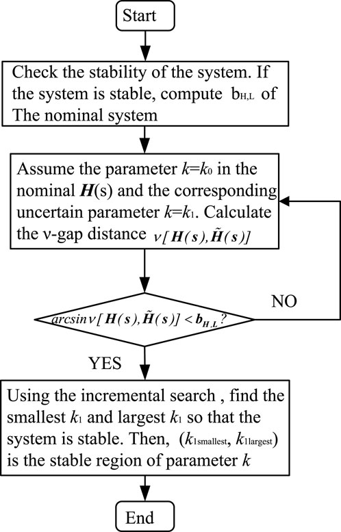
Figure 7. Flowchart of the algorithm of assessing the parameter stable region.
Step 1 Check the stability of the system. If the system is unstable, set bH,L = 0. Otherwise, compute bH,L of the nominal MIMO system in Figure 6A and continue.
Step 2 Assume the parameter k = k0 in the nominal H(s) and the corresponding uncertain parameter k = k1. Calculate the ν-gap distance
Step 3 If
Step 4 Using the incremental search, find the smallest k1 and the largest k1 so that the system is stable. Then the stable region for parameter k is (k1smallest, k1largest).
5 Simulation results
This section presents the simulation results to demonstrate the superiority of this method. We first calculate the robust stability margin of the MIMO system and compare with the results of eigenvalue analysis. Then, we present how to calculate the stable region of the parameters of PLL and Xg utilizing the method.
5.1 Relative stability evaluation
Recall the HVDC system connected with GSCs as shown in Figure 1. Common operation points and control parameters are provided in Supplementary Appendix SA. With five different sets of control parameters, we calculate the robust stability margin of the systems. The results are shown in Table 1. We can see that the second system has the largest robust stability margin, which means it has the best stability performance. The fifth system has the smallest robust stability margin, which indicates the worst stability performance.
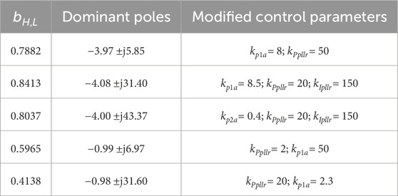
Table 1. Results of modal analysis and robust stability margin in DVC timescale.
Next, we compare the results with eigenvalue analysis. Table 2 shows the results of the eigenvalues and participation factors with two given sets of parameters. We can see that both of the two systems are stable since the eigenvalues are all in the left half plane. In addition, the real parts of the dominant poles of the two systems are close to each other. It seems that the relative stability of the systems are close. However, the relative stability of the systems are different according to the robust stability margin calculated by our proposed method. It can be verified by time-domain simulation based on detailed nonlinear model. According to the participation factors, kPpllr and kp1a have the greatest influence on the dominant poles of the two systems, respectively. Figure 8 shows the time domain response of θ3 of the rectifier with different kPpllr. When kPpllr changes from 2 to 0.05, the system remains stable. Figure 9 shows the time domain responses of θ1 of GSC 1 with different kp1a. When kp1a changes from 2.3 to 0.23, the system changes from stable to unstable. The results show that the system with kPpllr = 2 and kp1a = 50 can tolerate a larger range of parameter variation than the system with kPpllr = 20 and kp1a = 2.3, which means the former is more robust.

Table 2. Results of modal analysis in DC voltage control timescale.
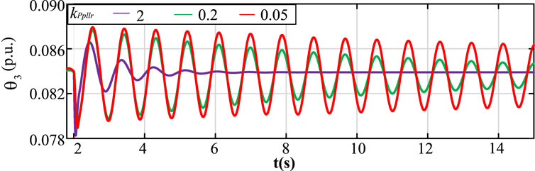
Figure 8. Time domain responses of θ3of the rectifier with different kPpllr.
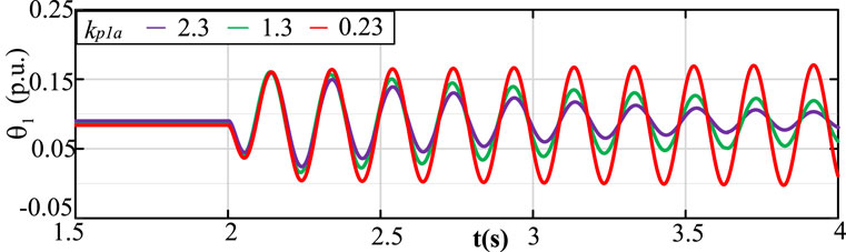
Figure 9. Time domain responses of θ1of GSC 1 with different kp1a.
5.2 Stable region of the parameters
In this subsection, we show how to calculate the stable region of the parameters of kp1a and Xg in the MIMO system.
First, we focuse on the proportional parameter kp1a of PLL control in GSC 1. Consider the MIMO system with parameters given in Supplementary Appendix SA. According to the expressions of robust stability margin (32), the robust stability margin of the system is 0.19. Based on the algorithm proposed in Section 2.3.2, when kp1a varies, we can compute the ν-gap
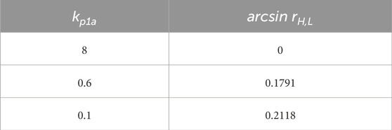
Table 3. Variation of arcsin rH,L under different parameters of kp1a.
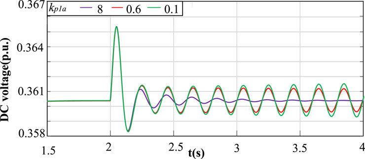
Figure 10. Nonlinear time-domain simulation.
Then, we compute the stable region of the reactance between the infinite bus and the point of interconnection Xg. As we know, Xg affects the short-circuit ratio (SCR) of the system. With the parameters shown in Supplementary Appendix SA (where Xg = 0.35), the robust stability margin of the system is 0.19. Table 4 shows the ν-gap ν-gap
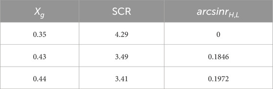
Table 4. Variation of SCR and arcsin rH,L under different parameters of Xg.

Figure 11. Nonlinear time-domain simulation.
The above two cases show the effectiveness of the proposed method to compute the stable regions of parameters. It is worth noticing that the results do not have conservatism since the stability criterion is a necessary and sufficient condition.
6 Conclusion
This paper analyzes the relative stability of a HVDC system connected with WFs utilizing the ν-gap metric. We build a MIMO system model of such a system represented by transfer function matrix. Then, a new stability index, which is called the robust stability margin, is proposed to assess the relative stability of a HVDC system connected with WFs. It can indicate how far the system is from instability. The larger the robust stability margin, the more stable the system performs. Next, a method to compute the stable region of control parameters is presented based on the sufficient and necessary stability criterion of the ν-gap metric. Simulations demonstrate the effectiveness of the proposed method. In future research, we would utilize this method to other MIMO systems containing renewable energies, for instance, to analyze the stability of a system with multiple wind turbines. Moreover, we will further explore parameter design methods for other MIMO systems to reach the maximize stability margin of the system.
Data availability statement
The original contributions presented in the study are included in the article/Supplementary Material, further inquiries can be directed to the corresponding author.
Author contributions
KJ: Data curation, Writing–review and editing. CY: Supervision, Writing–review and editing. WZ: Methodology, Supervision, Writing–original draft, Writing–review and editing. YC: Validation, Writing–original draft, Writing–review and editing. PX: Investigation, Methodology, Writing–review and editing. LL: Investigation, Methodology, Supervision, Writing–review and editing. PH: Investigation, Methodology, Supervision, Writing–review and editing.
Funding
The author(s) declare financial support was received for the research, authorship, and/or publication of this article. This work was partially supported by the science and technology project of State Grid Corporation of China, project number: 4000-202222070A-1-1-ZN, and partially by the National Natural Science Foundation of China under Grant 62303356.
Conflict of interest
The authors declare that the research was conducted in the absence of any commercial or financial relationships that could be construed as a potential conflict of interest.
The authors declare that this study received funding from State Grid Corporation of China. The funder had the following involvement: Data analysis and writing of the article.
Publisher’s note
All claims expressed in this article are solely those of the authors and do not necessarily represent those of their affiliated organizations, or those of the publisher, the editors and the reviewers. Any product that may be evaluated in this article, or claim that may be made by its manufacturer, is not guaranteed or endorsed by the publisher.
Supplementary material
The Supplementary Material for this article can be found online at: https://www.frontiersin.org/articles/10.3389/fenrg.2024.1379009/full#supplementary-material
References
Ángel Cardiel-Álvarez, M., Rodriguez-Amenedo, J. L., Arnaltes, S., and Montilla-Djesus, M. E. (2017). Modeling and control of lcc rectifiers for offshore wind farms connected by hvdc links. IEEE Trans. Energy Convers. 32, 1284–1296. doi:10.1109/TEC.2017.2696261
Bayhan, N., and Soylemez, M. T. (2007). “A new technique for calculation of maximum achievable gain and phase margins with proportional control,” in 2007 Mediterranean Conference on Control & Automation, China, 27-29 June 2007 (IEEE), 1–6.
Jiang, Y., Yu, W., Yu, W., and Wen, C. (2021). “On gradation and classification of faults for permanent magnet synchronous motor systems based on v-gap metric,”, China, 2021 IEEE 10th Data Driven Control and Learning Systems Conference (DDCLS) (IEEE).
Kovacevic, S., Jovcic, D., Despouys, O., and Rault, P. (2019). “Eigenvalue study of torsional interactions between gravelines generator and ifa2000 hvdc,” in 2019 20th International Symposium on Power Electronics (Ee), USA, 23-26 Oct. 2019 (IEEE), 1–6.
Liu, H., Shah, S., and Sun, J. (2014). “An impedance-based approach to hvdc system stability analysis and control development,” in 2014 International Power Electronics Conference (IPEC-Hiroshima 2014 ECCE-ASIA) (IEEE), China, 18-21 May 2014 (IEEE).
Liu, H., and Sun, J. (2013a). “Modeling and analysis of dc-link harmonic instability in lcc hvdc systems,” in 2013 IEEE 14th Workshop on Control and Modeling for Power Electronics (COMPEL) (IEEE), USA, 23-26 June 2013 (IEEE).
Liu, H., and Sun, J. (2013b). “Small-signal stability analysis of offshore wind farms with lcc hvdc,” in 2013 IEEE Grenoble Conference, China, 16-20 June 2013 (IEEE), 1–8.
Lu, J., Yuan, X., Hu, J., Zhang, M., and Yuan, H. (2020). Motion equation modeling of lcc-hvdc stations for analyzing dc and ac network interactions. IEEE Trans. Power Deliv. 35, 1563–1574. doi:10.1109/TPWRD.2019.2947572
Rohit, C., Darji, P. B., and Jariwala, H. (2021). “A stability assessment and estimation of equivalent damping gain for ssr stability by nyquist stability criterion in dfig-based windfarms,” in 2021 31st Australasian Universities Power Engineering Conference (AUPEC), USA, 26-30 Sept. 2021 (IEEE), 1–6.
Shen, J., Liu, C., Su, C., Li, H., and Wei, W. (2021). “Deepening research on state space analytical model of hvdc transmission system,” in 2021 IEEE 4th International Electrical and Energy Conference (CIEEC), China, 28-30 May 2021 (IEEE), 1–4.
Su, Y., Cao, R., Xin, Q., Xie, H., Liu, H., and Huang, W. (2023). “Equivalent impedance modeling of lcc-hvdc control system based on transfer function method,” in 2023 6th International Conference on Energy, Electrical and Power Engineering (CEEPE), USA, 12-14 May 2023 (IEEE), 813–818.
Sun, J. (2011). Impedance-based stability criterion for grid-connected inverters. IEEE Trans. Power Electron. 26, 3075–3078. doi:10.1109/TPEL.2011.2136439
Vinnicombe, G. (2001). Uncertainty and feedback. h ∞ loop-shaping and the ν-gap metric. IEEE. doi:10.1142/9781848160453
Wang, M., Chen, Y., Dong, X., Hu, S., Liu, B., Yu, S. S., et al. (2022a). Impedance modeling and stability analysis of dfig wind farm with lcc-hvdc transmission. IEEE J. Emerg. Sel. Top. Circuits Syst. 12, 7–19. doi:10.1109/JETCAS.2022.3144999
Wang, M., Li, Z., Dong, X., Liu, B., Su, W., and Zhang, X. (2020). “Sequence impedance modeling of dfig wind farm via lcc-hvdc transmission,” in 2020 Chinese automation congress (CAC) (IEEE) (New York: IEEE), 5320–5325.
Wang, X., Shi, P., Liu, Y., Nian, H., Chen, Z., and Chen, G. (2022b). “Impedance-based stability analysis of lcc-hvdc connected to weak grid considering frequency coupling characteristic,” in 2022 IEEE 5th International Electrical and Energy Conference (CIEEC) (IEEE), China, May 27 – 29, 2022 (IEEE), 153–157.
Yogarathinam, A., Kaur, J., and Chaudhuri, N. R. (2017). “Impact of inertia and effective short circuit ratio on control of frequency in weak grids interfacing lcc-hvdc and dfig-based wind farms,” in IEEE transactions on power delivery (Germany: IEEE), 2040–2051.
Yuan, H., Yuan, X., and Hu, J. (2017). Modeling of grid-connected VSCs for power system small-signal stability analysis in DC-link voltage control timescale. IEEE Trans. Power Syst. 32, 3981–3991. doi:10.1109/tpwrs.2017.2653939
Zhou, H., Yang, G., and Wang, J. (2011). Modeling, analysis, and control for the rectifier of hybrid hvdc systems for dfig-based wind farms. IEEE Trans. Energy Convers. 26, 340–353. doi:10.1109/TEC.2010.2096819
Keywords: wind farms, HVDC, ν-gap metric, robust stability margin, stable region
Citation: Jiang K, Ye C, Zheng W, Chen Y, Xiong P, Li L and Hu P (2024) Relative stability evaluation of HVDC-connected wind farms. Front. Energy Res. 12:1379009. doi: 10.3389/fenrg.2024.1379009
Received: 30 January 2024; Accepted: 30 May 2024;
Published: 16 July 2024.
Edited by:
Juan Carlos Jauregui, Autonomous University of Queretaro, MexicoReviewed by:
Joshuva Arockia Dhanraj, Dayananda Sagar University, IndiaYunhui Huang, Wuhan University of Technology, China
Li Sun, Harbin Institute of Technology, Shenzhen, China
Copyright © 2024 Jiang, Ye, Zheng, Chen, Xiong, Li and Hu. This is an open-access article distributed under the terms of the Creative Commons Attribution License (CC BY). The use, distribution or reproduction in other forums is permitted, provided the original author(s) and the copyright owner(s) are credited and that the original publication in this journal is cited, in accordance with accepted academic practice. No use, distribution or reproduction is permitted which does not comply with these terms.
*Correspondence: Wanning Zheng, emhlbmd3YW5uaW5nQHd1c3QuZWR1LmNu