Accurate parameters identification of proton exchange membrane fuel cell using Young’s double-slit experiment optimizer

Introduction: Fuel cell technology is a harbinger of the future for generating electricity due to their high efficiency and low emissions achieved through the direct conversion of chemical energy into electrical energy without combustion.

Methods: To optimize the design and performance, a fuel cell model is essential to predict its behaviour in different conditions. This technical note presents a novel physics-based approach, the Young’s Double-slit Experiment Optimizer (YDEO), for identifying parameters in Proton Exchange Membrane Fuel Cells. A performance metric is established by formulating an objective function that relies on the summation of squared errors between experimental and estimated values.

Results and discussion: The effectiveness of this approach is evaluated through the analysis of four benchmark test cases: Horizon 500 W, BCS500 W, NedstackPS6, and 250 W. The corresponding objective function values for these test cases are 0.011243, 2.065557, 0.011698, and 5.250849, respectively. The simulation results demonstrate the efficacy of the proposed YDEO algorithm when compared with other existing popular and contemporary algorithms in the literature.

1 Introduction

1.1 Motivation

Fossil fuel-based transportation has several drawbacks which have significant environmental and economic impact (Carrette et al., 2000), (Ahluwalia and Wang, 2008), (Pan et al., 2021), (Sharaf and Orhan, 2014), (Zhou et al., 2024). The burning of fossil fuels releases greenhouse gases such as carbon dioxide, which contribute to climate change and air pollution. These resource fuels are non-renewable resources which means they will eventually run out. Extracting and transporting the fossil fuels can be environmentally damaging and the prices of fossil fuels can be unpredictable as they are subject to global market forces making it difficult for businesses and consumers to accommodate budget for fuel expenses. Many Nations rely heavily on fossil fuels that they import, making them susceptible to fluctuations in prices and disruptions in the supply chain. Burning fossil fuels and resulting air pollution can harm human health, especially those residing in urban regions (Zhang et al., 2016), (Ma et al., 2023), (Zhu et al., 2024). Additionally, fossil fuel based transportation is not as energy efficient as electric vehicles owing to higher consumption of fossil fuel and thereby higher costs.

The use of fuel cell technology has the potential to transform transportation by offering a clean and effective substitute to conventional fossil fuel-based vehicles (Bai et al., 2022). Fuel cells convert chemical energy from a fuel source, such as hydrogen, into electrical energy to power an electric motor. This results in zero emissions and high energy efficiency. Additionally, fuel cells can have a longer range and faster refuelling times compared to battery-electric vehicles. However, the widespread adoption of fuel cell technology in transportation is currently limited by the cost and availability of hydrogen fuel infrastructure.

There are various types of fuel cell technologies, including alkaline fuel cells, molten carbonate fuel cells, solid oxide fuel cells, phosphoric acid fuel cells, and Proton Exchange Membrane fuel cells. PEMFC is a popular technology due to its low operating temperature, high power density, fast startup, and low emissions (Wang et al., 2011). PEMFC operates at temperatures between 60°C–100°C, making it suitable for various applications, including automotive, residential, and portable power.

A fuel cell’s mathematical model is essential for various reasons. Firstly, it allows engineers and researchers to simulate and predict how a fuel cell would behave under different operating conditions such as temperature, pressure, or fuel composition. This helps them to optimize the design and working of the fuel cell to make it more efficient, durable, and cost-effective. Additionally, a mathematical model can provide insights into the physical and chemical processes that take place within the fuel cell. Understanding of these processes will benefit the researchers to develop new materials, catalysts and operating strategies so to enhance its performance. Moreover, a mathematical model can be used to simulate the interactions between a fuel cell and other components like battery or an electric motor that are present in the entire system. This information can be leveraged to enhance the overall performance and efficiency of the system. Mathematical models can also evaluate the economic feasibility of different fuel cell designs and configurations, as well as the potential cost savings of using fuel cells instead of traditional fossil fuels.

Fuel cell modelling approaches can be broadly classified into three categories:

Empirical models: These models are based on an experimental data and are used to predict the performance of a fuel cell under different operating conditions. They are relatively simple to develop and can provide good predictions for specific operating conditions, but they may not be accurate for conditions that are different from the ones used to develop the model.

Physics-based models: These models are employed to comprehend the fundamental mechanisms of a fuel cell and have the potential to forecast the performance of a fuel cell across a broad spectrum of operating circumstances. They are more complex to develop and require a good understanding of the underlying physics of the fuel cell, but they provide more accurate predictions than empirical models.

Hybrid models: These models combine both empirical and physics-based approach, often taking advantage of the strengths of both models, to develop a more accurate model.

The choice of modelling approach depends on the specific application and the level of details and accuracy required.

The need for estimation of fuel cell model parameters arises due to the complexity and variability of fuel cell systems. Fuel cell systems are highly non-linear, dynamic, and dependent on many factors such as temperature, humidity, pressure, and fuel composition. These factors can affect the performance of the fuel cell and make it difficult to predict the behaviour of the system based on the sole approach of theoretical models. Estimation of fuel cell model parameters addresses these issues by using experimental data to estimate the unknown parameters of the model. Utilizing experimental data for parameter estimation allows the model to be calibrated, aligning its predictions with the actual system’s behavior and consequently enhancing the accuracy of predictions.

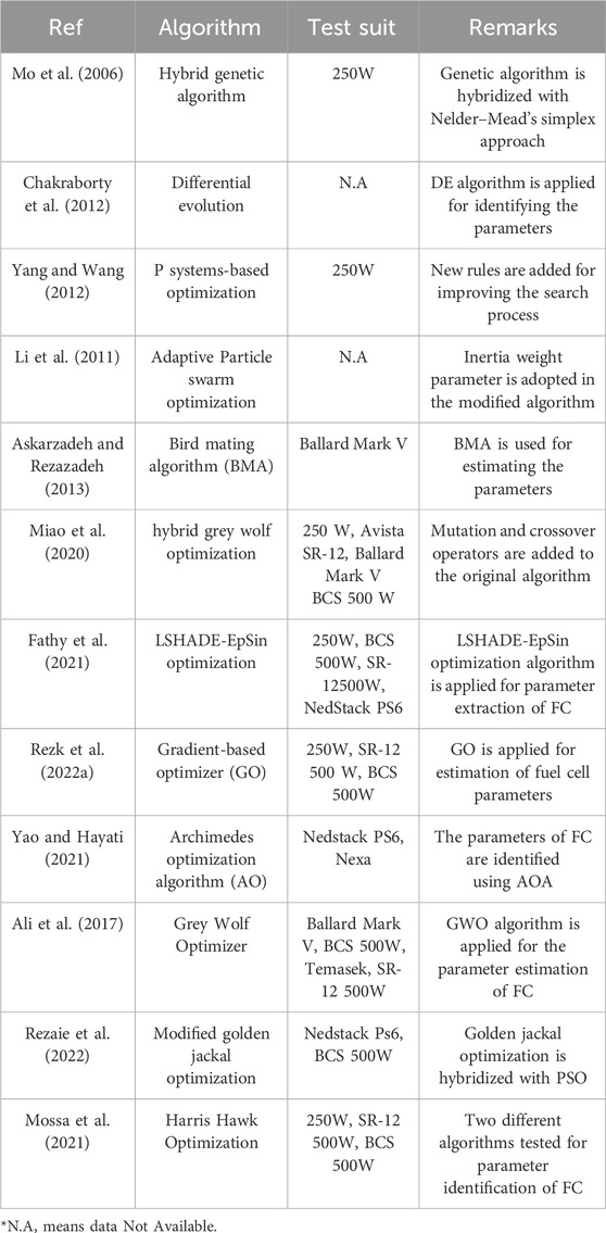
Meta-heuristic optimization algorithms are important for fuel cell parameter estimation because they provide a powerful tool for solving the complex and non-linear optimization problem of estimating the parameters of a FC model.

FC model is highly non-linear and have multiple local minima and maxima in the parameter space, making it difficult for conventional optimization algorithms such as gradient-based methods to find the global optimum solution. Meta-heuristic optimization algorithms, on the other hand, are designed to explore a large search space and are able to find global optimal solutions in non-convex problems.

Existing meta-heuristic algorithms for parameter estimation of fuel cell models have a few drawbacks, including:

Sensitivity to initial conditions: Meta-heuristic algorithms are often sensitive to the initial conditions, meaning that the final solution can be different depending on the initial values of the parameters. This can make it difficult to obtain a consistent and reliable solution for the parameter estimation problem.

Convergence to local optima: Meta-heuristic algorithms, like other optimization algorithms, can sometimes converge to local optima rather than the global optimum solution. This can be a problem in fuel cell parameter estimation, as the parameter space is often highly non-linear and has multiple local minima and maxima.

Difficulty in handling constraints and bounds: Some meta-heuristic algorithms face challenges during handling of constraints and boundaries on the parameters which can make it difficult to find the global optimum solution while satisfying the constraints and bounds.

Slow convergence: Some meta-heuristic algorithms can be slow to converge to the global optimum solution, especially when the parameter space is large or complex. This can make it impractical to use these algorithms for real-time parameter estimation in a fuel cell system.

Lack of robustness: Some meta-heuristic algorithms lack robustness and can be affected by the presence of outliers or other anomalies in the data.

High-computational burden: Some algorithms are highly complex and requires huge mathematical calculations and hence computational burden.

To overcome the limitations, this article introduces a novel method for estimating parameters of FC based on Young’s double-slit experiment. The proposed approach for parameter extraction from practical measurement data is assessed using four benchmark test cases and compared with several algorithms from the literature. The comparative analysis demonstrates the robustness and effectiveness of the proposed method.

2 Mathematical model of PEMFC

A PEMFC can transform the stored chemical energy in a fuel like hydrogen, and an oxidizing agent such as oxygen taken from the atmosphere, into electrical energy without any intermediaries (Qin et al., 2020)– (Abd Elaziz et al., 2023), (Ayyarao et al., 2024) (Askarzadeh and Rezazadeh, 2012; Priya et al., 2018; Yuan et al., 2020; Duan et al., 2022). The working of FC is illustrated in Figure 1. The overall reaction occurring in a PEMFC can be represented using Equation 1.

$2H_2+O_2\to 2H_{2}O(1)$

Figure 1

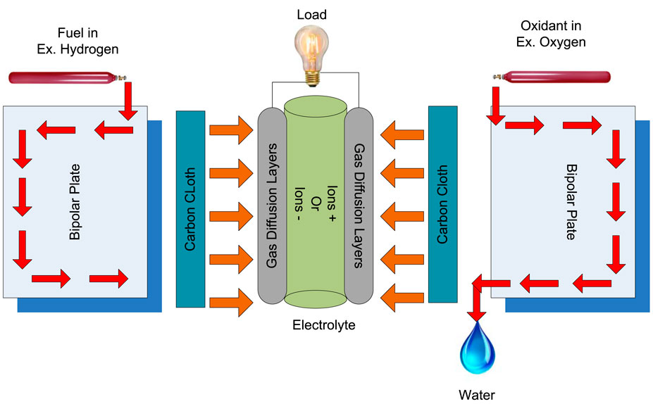
Figure 1. Working of fuel cell- conceptual view.

This reaction produces a voltage between the two electrodes, which can be used to power an external circuit. The PEMFC consists of a cathode (positive electrode), an anode (negative electrode), and a proton exchange membrane (PEM) in between them.

The anode half-cell reaction in a PEMFC can be represented using Equation 2.

$2H_2\to 4e^{-}+4H^{+}(2)$

This reaction releases hydrogen ions (protons) and electrons, which flow through separate paths to the cathode and the electrons drift through an external circuit, producing electrical energy. The protons travel through the PEM, which is a thin, solid polymer electrolyte that allows only the passage of protons. The protons combine with the oxygen and electrons at the cathode, which can be represented using Equation 3.

$4e^{-}+4H^{+}+O_2\to 2H_{2}O(3)$

The polarization curve illustrates the relationship between the output voltage and the current density, revealing the non-linear output characteristics of a PEMFC. Under standard conditions (298.15 K and 1 bar), the optimal thermodynamic potential of an H2/O2 PEMFC is approximately 1.229 V.

The voltage produced by a PEMFC is determined by the difference in electrochemical potential between the anode and cathode. This is typically expressed in terms of the standard electrode potential of each half-reaction. The overall voltage (V) produced by the cell can be calculated using the Nernst equation:

The overall voltage of the stack is given as:

${V=N}_{cell}{V}_{cell}(4)$

The cell voltage $V_{cell}$ is calculated using (Equation 4).

$V_{cell}=E_{Nernst}-V_{act}-V_{ohm}–V_{con}(5)$

The cell voltage given in (Equation 5) can be obtained by obtaining each term on the R.H.S.

The modified Nernst voltage can be obtained by considering the effect of temperature and pressure changes, relative to the standard conditions of 298.15 K and 1 bar, as described in Equation 6.

$E_{Nernst}=1.229-85\times {10}^{-5}\left(T-298.15\right)+430.85\times {10}^{-7}T\left[\ln \left(P_{H_2}\sqrt{P_{O_2}}\right)\right](6)$

Equations 7, 8 can be used to obtain the partial pressures $\left\{{\mathrm{P}}_{H_2},{\mathrm{P}}_{{\mathrm{O}}_2}\right\}$, if the reactants are ${\mathrm{H}}_2$ and ${\mathrm{O}}_2$. If the reactants are air and ${\mathrm{H}}_2$, then ${\mathrm{P}}_{{\mathrm{O}}_2}$ should be calculated using (Equation 9).

${\mathrm{P}}_{H_2}=\frac{{\mathrm{R}}_{Ha}{\mathrm{P}}_{{\mathrm{H}}_2\mathrm{O}}}{2}\left[{\left(\exp \left(\frac{1.635}{T^{1.334}}\frac{I}{A}\right)\frac{{\mathrm{R}}_{Ha}{\mathrm{P}}_{{\mathrm{H}}_2\mathrm{O}}}{P_a}\right)}^{-1}-1\right](7)$

${\mathrm{P}}_{{\mathrm{O}}_2}={\mathrm{R}}_{Hc}{\mathrm{P}}_{{\mathrm{H}}_2\mathrm{O}}\left[{\left(\exp \left(\frac{4.192}{T^{1.334}}\frac{I}{A}\right)\frac{{\mathrm{R}}_{Hc}{P}_{H20}}{P_C}\right)}^{-1}-1\right](8)$

${\mathrm{P}}_{{\mathrm{O}}_2}=\frac{{\mathrm{P}}_{\mathrm{c}}-\mathrm{R}{\mathrm{H}}_{\mathrm{c}}{\mathrm{P}}_{{\mathrm{H}}_2}\mathrm{o}}{\left(1+\frac{0.79}{0.21}\right)\exp \left[\frac{0.291}{{\mathrm{T}}^{0.832}}\frac{\mathrm{I}}{\mathrm{A}}\right]}(9)$

${\mathit{log}}_{10}\left(P_{H_{2}O}\right)=29.5\times {10}^{-3}\left(∆T\right)-91.8\times {10}^{-6}{\left(∆T\right)}^2+14.4\times {10}^{-8}{\left(∆T\right)}^3-2.18(10)$

Where $∆T=T-273.15$

It is possible to calculate $V_{act}$ using a semiempirical equation, which can be expressed in the following way:

$V_{act}=-\left[{\xi }_1+{\xi }_{2}T+{\xi }_{3}Tln\left(C_{O_2}\right)+{\xi }_{4}Tln\left(I\right)\right](11)$

The concentration of dissolved oxygen at the cathode’s catalytic interface, $C_{O_2}$, can be determined using Henry’s Law

$C_{O_2}=\frac{P_{O_2}}{5.08\times {10}^6}\mathit{exp}\left(\frac{498}{T}\right)(12)$

The voltage $V_{ohm}$ that appears across the resistances $R_m$ and $R_c$ can be determined by applying Equation 13, and it shows a linear relationship with the current flowing through the system

$V_{ohm}=I\left(R_m+R_c\right)(13)$

$R_m=\frac{{\rho }_m.l}{A}(14)$

The specific resistance can be formulated using (Equation 15).

${\rho }_m=\frac{181.6\left[1+0.03\left(\frac{I}{A}\right)+0.062{\left(\frac{T}{303}\right)}^2{\left(\frac{I}{A}\right)}^{2.5}\right]}{\left[\lambda -0.634-3\left(\frac{I}{A}\right)\right]\mathit{exp}\left[4.18\left(\frac{T-303}{T}\right)\right]}(15)$

The voltage drop $V_{con}$ caused by concentration changes can be described using an empirical equation presented in (Equation 16).

$V_{con}=-Bln\left(1-\frac{J}{J_{\mathit{max}}}\right)=-Bln\left(1-\frac{\frac{I}{A}}{J_{\mathit{max}}}\right)(16)$

To accurately predict the performance of the PEMFC stack, it is necessary to estimate the values of its seven parameters. The objective function is a key tool in this process, as it enables the identification of unknown parameters through the comparison of experimental and simulated data. In particular, an objective function is created by summing the squared differences between the measured and simulated values using Equation 17.

$F_{obj}={\displaystyle {\sum }_{i=1}^N}{\left(V_{sim}-V_{\mathit{exp}}\right)}^2(17)$

The step-by-step procedure to calculate the stack voltage is outlined as:

i. Begin by defining all constants such as l, A, T, P_H2, P_O2, J_max,

ii. Obtain the variable parameters ${\xi }_1,{\xi }_2,{\xi }_3,{\xi }_4,\lambda ,R_c,\mathrm{B}$ from the optimization algorithm

iii. Calculate the saturation pressure of water using (Equation 10).

iv. Compute $C_{O_2}$ using (Equation 12).

v. Determine $R_m$ and ${\rho }_m$ using (Equations 14, 15) respectively.

vi. Calculate the voltage drop $V_{con}$ using (Equation 16), $V_{ohm}$ using (Equation 13), $V_{act}$ using (Equation 11), $E_{Nernst}$ using (Equation 6).

vii. Now, compute the cell voltage using (Equation 5) and finally, derive the stack voltage using (Equation 4).

The MATLAB code to calculate the objective function is publicly available on the MathWorks website, associated with article (Ayyarao et al., 2024). Interested users can reference this code for a basic understanding of the concept.

3 Young’s double-slit experiment optimization

3.1 Inspiration

Young’s double-slit experiment optimization is an optimization algorithm that takes inspiration from the well-known double-slit experiment conducted by Thomas Young during the early 1800 s. The experiment entailed directing a beam of light through two slender openings in a barrier, leading to the observation of an interference pattern on a screen positioned behind the barrier. Unlike lasers, which emit monochromatic and coherent light, most lights are non-monochromatic and incoherent. The experiment is quite straightforward and revolves around the principle of illuminating a barrier containing two small slits—the first and second slits—with light from a monochromatic source. Beyond the barrier, a projection screen is meticulously positioned to document the trajectory of light. Upon passing through the narrow slits, the light waves intersect, giving rise to an interference pattern discernible on the screen. This phenomenon engenders semicircular waves as light traverses the slits, wherein luminous bands (fringes) denote interference maxima and dim bands signify interference minima. The interference pattern persists uniformly across the screen, with the positions of bright and dark fringes remaining constant. Notably, maintaining coherence between the two light sources is imperative for ensuring the stability of the interference pattern.

3.2 Mathematical model

The Young’s double-slit experiment optimizer is based on the concept of interference patterns, like those observed in Young’s experiment (Abdel-Basset et al., 2023). The various steps involved in YDEO algorithm are:

3.2.1 Initialization

In the first phase of the experiment, a group of monochromatic light waves are created using Equation 18.

$X=Lb+rand\left(1,N\right).\times \left(Ub-Lb\right)(18)$

3.2.2 Huygen’s Principle

According to Huygen’s principle, each point on a wavefront behaves as a generator of secondary wavelets that spread uniformly in all directions at a constant speed. The combination of these wavelets determines the position of the new wavefront later given in Equations 19, 20.

${FS}_i=X_i+L\times rand\left(-1,1\right)\times \left(\frac{1}{N}{\displaystyle {\sum }_{j=1}^N}{X}_j-X_i\right)(19)$

${SS}_i=X_i-L\times rand\left(-1,1\right)\times \left(\frac{1}{N}{\displaystyle {\sum }_{j=1}^N}{X}_j-X_i\right)(20)$

3.2.3 Travelling waves update

During Young’s double-slit experiment, the passage of coherent light through two slits produces an interference pattern on a screen located behind the slits. In Young’s double-slit experiment, the coherent light passing through the two slits creates two sets of waves that interfere with each other. The resultant wave creates a pattern of bright and dark fringes on the screen, which correspond to areas of constructive and destructive interference.

$X_i=\left(\frac{{FS}_i+{SS}_i}{2}\right)+\left\{\begin{array}{l}\begin{array}{cc}0& ifCIhappensatm=0\end{array}\\ \begin{array}{cc}\left(2m+1\right)\frac{\rho }{2}& ifDIhappenswhenmisodd\end{array}\\ \begin{array}{cc}3\rho & ifDIhappenswhenmiseven\end{array}\end{array}\right.(21)$

Here $m=i-1$

3.2.4 Wave fringes

When the light waves from the pair of slits intersect on the screen, they undergo constructive or destructive interference. Constructive interference occurs where the waves are in phase, meeting crest-to-crest or trough-to-trough, resulting in a bright band. Conversely, destructive interference occurs when the waves meet crest-to-trough, leading to a dark band. The spacing of these light and dark bands is determined by factors such as the distance between the slits and the screen, along with the wavelength of the light employed. The pattern of bands can be explained using the principles of wave interference.

3.2.5 Constructive interference

CI is the phenomenon where waves combine to produce a larger amplitude. In the case of Young’s double-slit experiment, constructive interference occurs when the waves of light passing through the two slits are in phase with each other. This occurs because the waves from each slit arrive at the screen with a path difference. When the path difference is equal to an integer multiple of the wavelength of the light, the waves interfere constructively, creating a bright fringe. The path difference is determined by the distance between the slits and the distance from the slits to the screen.

In the case of (i is even), the wave update is given by Equation 22.

$X_i^{t+1}=X_i^t-\left(\left(1-r_1\right)\times \frac{2}{1+\sqrt{\left|1-{\beta }^2\right|}}\times {\mathit{Int}}_i^{t+1}\times X_i^t-r_1\times \left(X_{rand1}^t-X_{rand2}^t\right)\right))(22)$

In the case of i = 0, the wave update is given by Equation 23.

$X_i^{t+1}=X_i^t+\left(\frac{2}{1+\sqrt{\left|1-{\beta }^2\right|}}\times {\mathit{Int}}_{\mathit{max}}^{t+1}\times X_i^t-r_2\times z\times X_{rand3}^t\right)(23)$

3.2.6 Destructive interference

DI happens when the crests of one wave coincide with the troughs of another wave, resulting in a reduction in the overall amplitude (brightness) of the interference pattern. In the context of the double-slit experiment, the light passing through each slit generates its own wave pattern, which then overlap and interfere with each other on the screen. When the crest of one wave coincides with the trough of another wave, the two waves cancel each other out, resulting in a dark spot on the screen where no light is detected and this given by Equation 24.

$X_i^{t+1}=X_i^t-\left(r_1\times 0.38\times {\mathit{tanh}}^{-1}\left(-\frac{t}{t\_\mathit{max}}+1\right)\times {\mathit{Int}}_i^{t+1}{\times X}_i^t-\frac{t^{2\times r_2}}{V}{X}_B^t\right)(24)$

The flowchart for YDEO algorithm for fuel cell parameter estimation is illustrated in Figure 2.

Figure 2

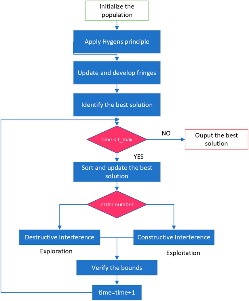
Figure 2. Flowchart of YDEO algorithm.

4 Results and discussion

As mentioned in Section 2, the PEMFC model requires the estimation of seven unknown parameters. The bounds of the parameter space for all the test cases can be found in Table 1, while the testing conditions for the three benchmark systems are itemized in Table 2. To identify the parameters of the PEMFC model for the Horizon500W, BCS500W, and NedstackPS6 benchmarks, we proposed the YDEO algorithm, which was implemented in MATLAB and executed on an Intel I5 processor. We compared the performance of the proposed YDEO algorithm with that of other recent and contemporary optimization algorithms, including Particle Swarm Optimization (Kennedy and Eberhart, 1995), Multi-Verse Optimization (MVO) (Mirjalili et al., 2016), Slime-Mould Optimization (SMO) (Li et al., 2020), Harris Hawk Optimization (HHO) (Heidari et al., 2019), Arithmetic Optimization Algorithm (AOA) (Abualigah et al., 2021), Grey Wolf Optimization (GWO) (Mirjalili et al., 2014), Artificial Electric Field Algorithm (Anita and Yadav, 2019), and Artificial Vulture Optimization Algorithm (Abdollahzadeh et al., 2021). For all algorithms, a population size of 50 was utilized, and the maximum allowable number of function evaluations was established at 5000.

Table 1

Table 1. Bounds of the parameter space.

Table 2

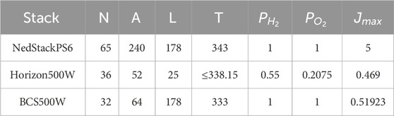
Table 2. Testing conditions for various PEMFC stacks.

4.1 Horizon500W results

Figure 3 depicts the convergence curves of the YDEO algorithm, as well as those of other algorithms. This graph showcases the superior performance of the algorithm in terms of both accuracy and convergence speed. Figure 4 depicts the polarization curve with experimental and calculated values. This graph clearly shows that the simulated values are very closer to the experimental values. Experimental measurements and estimated values for the first test case are recorded in Table 3. The overall SSE value for this test case is 0.011243. The maximum and minimum absolute error between experimental and simulated values are 5.621E-02 and 4.950E-04 respectively. The sum of the absolute error values is equal to 3.189E-01 which is very less and hence the mathematical model is very closely mimics the practical system.

Figure 3

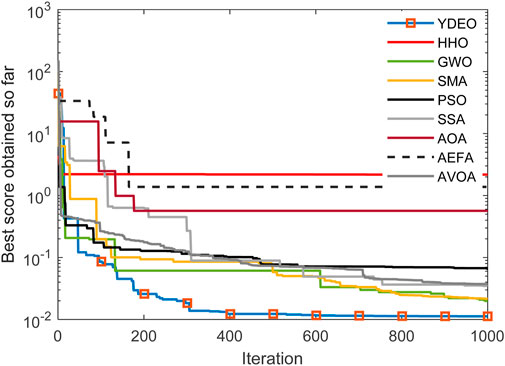
Figure 3. Convergence curve of YDEO when compared with other algorithms in the case of Horizon500W fuel cell.

Figure 4

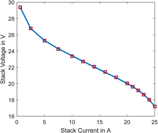
Figure 4. Horizon500W polarization curve with experimental and calculated values.

Table 3

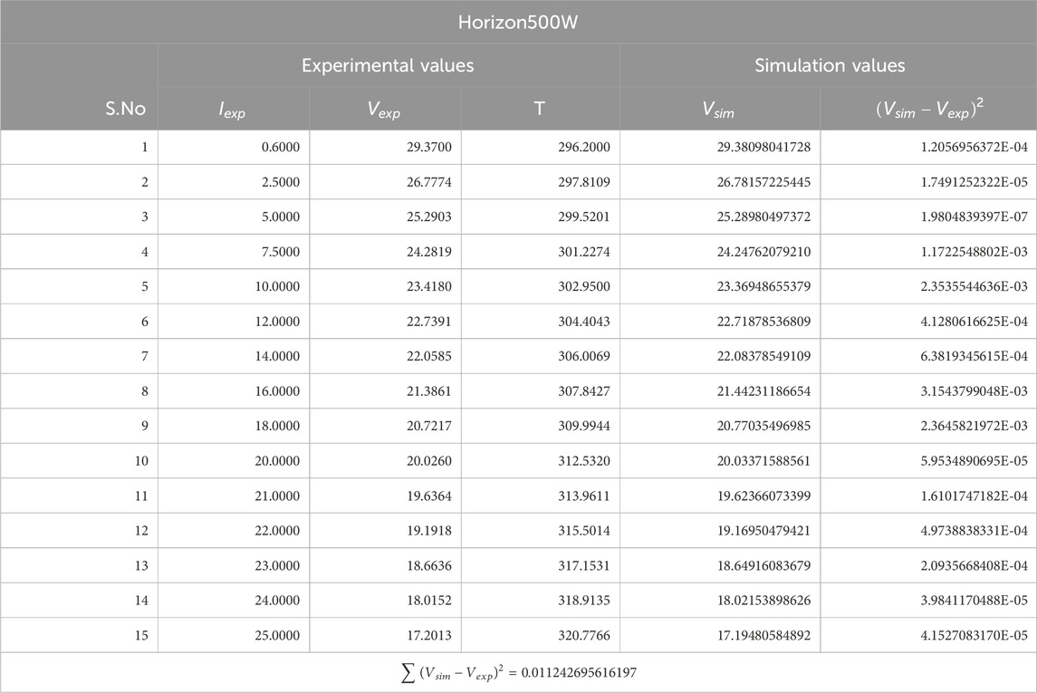
Table 3. Experimental and simulated values for Horizon500W.

4.2 NedstackPS6 results

Figure A1 in appendix illustrates the convergence performance of YDEO algorithm when compared with the recent algorithms and the graphs reveal that the proposed YDEO algorithm achieves minimum objective function value with less iterations. Table 4 records the experimental and simulated values. The overall SSE values for the second test case is 2.065557. The maximum and minimum absolute error between the measured and simulated values are 7.158E-01 and 1.356E-02 respectively and the sum of the absolute error values is 5.945. Figure 5 illustrates the polarization curve with the experimental data and estimated data using the proposed algorithm. To exemplify NedStack’s performance across varied simulated cell temperature conditions, we’ve visually represented the impact of temperature fluctuations in a Figure A2 found in the appendix. The findings reveal a notable trend: as the temperature increases, there’s a corresponding rise in stack voltage.

Table 4

Table 4. NedstackPS6 experimental and simulated results.

Figure 5

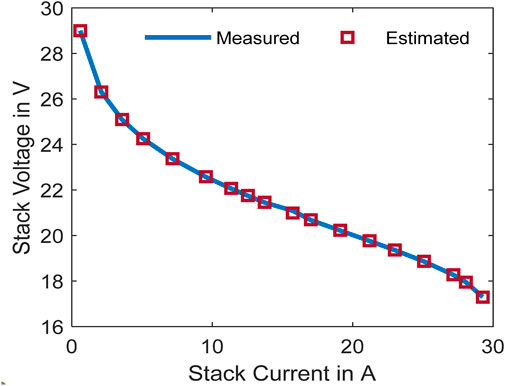
Figure 5. Polarization curve for BCS500W.

4.3 BCS500W results

Figure A3 depicts how the YDEO algorithm compares to recent algorithms in terms of convergence performance. The graphs demonstrate that the YDEO algorithm achieves a lower objective function value with fewer iterations. Meanwhile, Table 5 presents both experimental and simulated values. For the third test case, the overall sum of squared errors is 0.011698. The maximum and minimum absolute errors between measured and simulated values are 7.158E-01 and 1.356E-02, respectively. The total sum of absolute error values amounts to 5.945.

Table 5

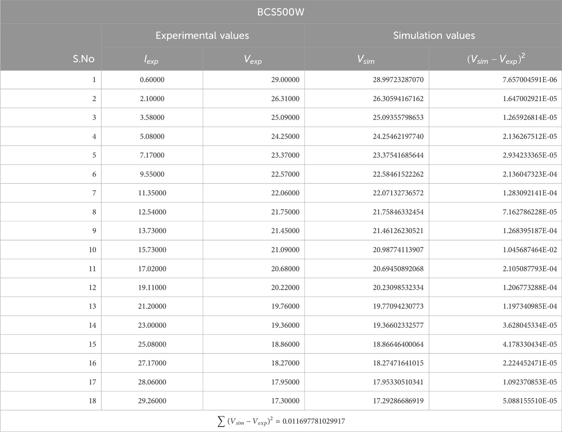
Table 5. BCS500W stack results.

4.4 Robustness to varying pressures and temperatures

The effectiveness of the proposed algorithm underwent scrutiny through thorough analysis of a vast 250W PEMFC dataset, covering diverse data points from various temperature and pressure configurations. Moreover, Figure 6 illustrates polarization curves, displaying the experimental and predicted stack voltages at two distinct sets of conditions: 3/5 bar pressure and 353.15 K temperature, and 1/1 bar pressure and 343.15 K temperature. These curves unveil nuanced distinctions between the experimental and predicted values. Additionally, Table 6 provides a comprehensive overview of the experimental data juxtaposed with the estimated data generated through the proposed method.

Figure 6

Figure 6. Polarization curves for 250W benchmark model.

Table 6

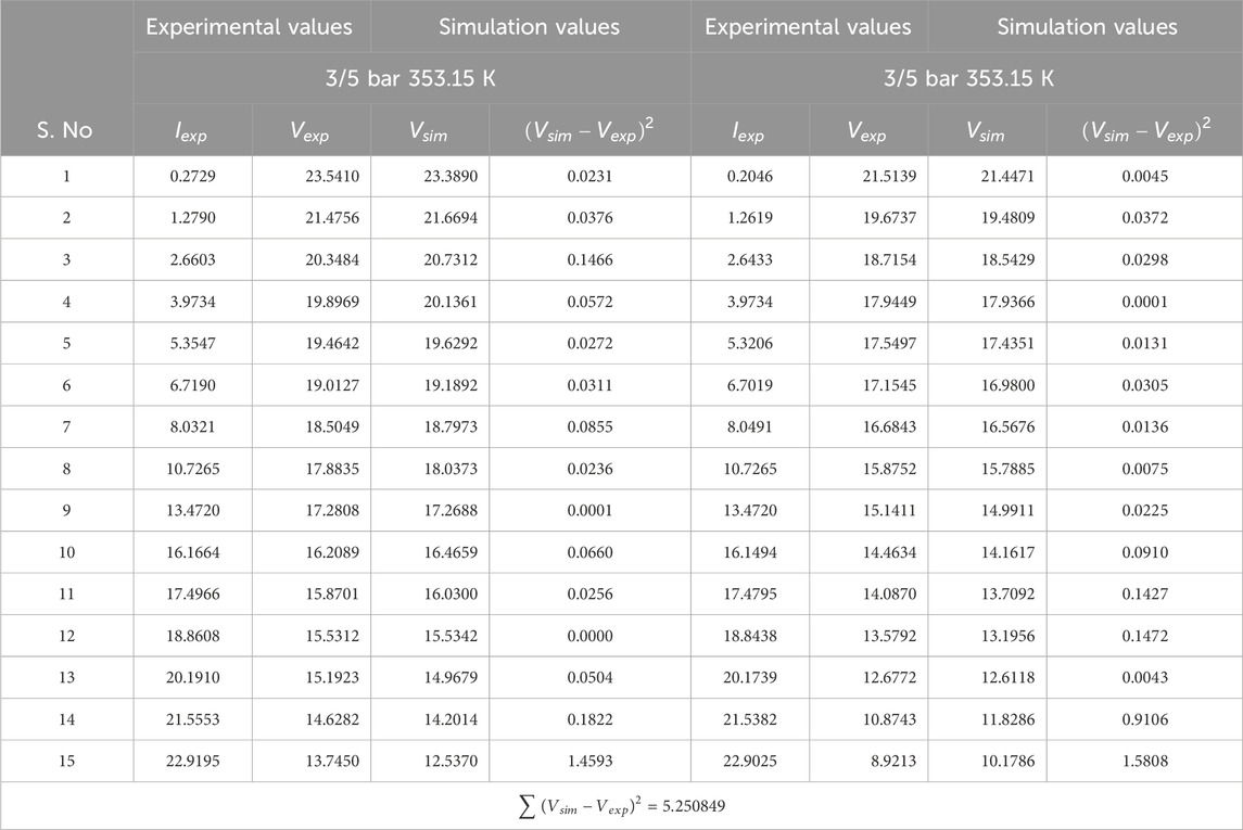
Table 6. Benchmark model 250W stack results.

4.5 Comaprison with other algorithms

The proposed method’s efficacy is demonstrated through comparison with existing algorithms in the literature, utilizing three distinct datasets. These comparisons are quantified through the evaluation of an objective function, specifically the SSE between experimental and estimated voltages. The results, neatly organized in a Table 7, unequivocally showcase the superiority of the proposed algorithm across all three test cases. With its consistently lower objective function values, the proposed method emerges as the standout performer, surpassing the alternatives examined in the study. This outcome not only underscores the effectiveness of the novel approach but also positions it as a leading contender for fuel cell parameter estimation, potentially offering significant advancements in this domain.

Table 7

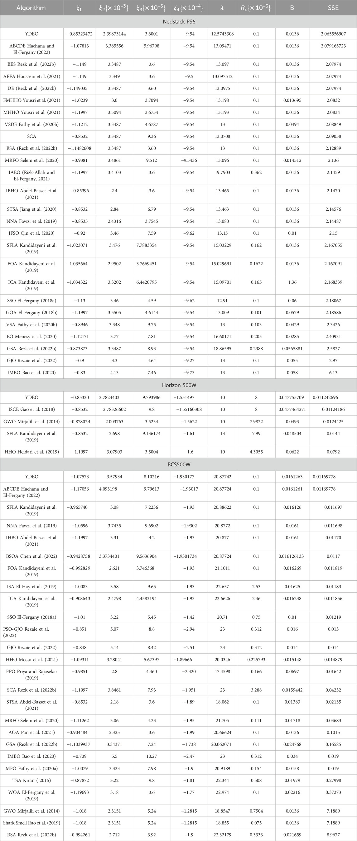
Table 7. Comparison of YDEO with other algorithms for NedstackPS6, Horizon 500W, BCS500W.

5 Conclusion

The estimation of unknown model parameters is a challenging but crucial topic in the research of PEMFC. This study has proposed a new and accurate approach, namely, the Youngs Double slit Experiment Optimization algorithm, to address this issue. This approach can greatly benefit the design, simulation, analysis, evaluation, and control of PEMFC systems. By formulating an objective function based on the sum of squared errors between experimental and calculated values, this study has evaluated the YDEO algorithm on four benchmark test cases: Horizon 500W, BCS500W, NedstackPS6 and 250 W. The simulation outcomes indicate that the YDEO algorithm, as suggested, surpasses other widely used and current algorithms found in literature. This positions it as a promising tool for accurately estimating parameters in PEMFC models.

This work can be extended by combining mathematical model with machine learning algorithms for bridging the gap between theory and practical.

Data availability statement

The original contributions presented in the study are included in the article/supplementary material, further inquiries can be directed to the corresponding author.

Author contributions

AT: Conceptualization, Data curation, Formal Analysis, Investigation, Methodology, Project administration, Resources, Software, Supervision, Visualization, Writing–original draft, Writing–review and editing. NP: Conceptualization, Data curation, Formal Analysis, Investigation, Methodology, Resources, Software, Supervision, Visualization, Writing–original draft, Writing–review and editing. BK: Conceptualization, Data curation, Formal Analysis, Investigation, Methodology, Resources, Software, Supervision, Visualization, Writing–original draft, Writing–review and editing. AA: Conceptualization, Data curation, Formal Analysis, Investigation, Methodology, Resources, Software, Supervision, Visualization, Writing–original draft, Writing–review and editing.

Funding

The author(s) declare that no financial support was received for the research, authorship, and/or publication of this article.

Conflict of interest

Author NP was employed by the Bharat Heavy Electricals Ltd.

The remaining authors declare that the research was conducted in the absence of any commercial or financial relationships that could be construed as a potential conflict of interest.

Publisher’s note

All claims expressed in this article are solely those of the authors and do not necessarily represent those of their affiliated organizations, or those of the publisher, the editors and the reviewers. Any product that may be evaluated in this article, or claim that may be made by its manufacturer, is not guaranteed or endorsed by the publisher.

References

Abd Elaziz, M., Abualigah, L., Issa, M., and Abd El-Latif, A. A. (2023). Optimal parameters extracting of fuel cell based on Gorilla Troops Optimizer. Fuel 332, 126162. doi:10.1016/j.fuel.2022.126162

CrossRef Full Text | Google Scholar

Abdel-Basset, M., El-Shahat, D., Jameel, M., and Abouhawwash, M. (2023). Young’s double-slit experiment optimizer : a novel metaheuristic optimization algorithm for global and constraint optimization problems. Comput. Methods Appl. Mech. Eng. 403, 115652. doi:10.1016/j.cma.2022.115652

CrossRef Full Text | Google Scholar

Abdel-Basset, M., Mohamed, R., Elhoseny, M., Chakrabortty, R. K., and Ryan, M. J. (2021). An efficient heap-based optimization algorithm for parameters identification of proton exchange membrane fuel cells model: analysis and case studies. Int. J. Hydrogen Energy 46 (21), 11908–11925. doi:10.1016/j.ijhydene.2021.01.076

CrossRef Full Text | Google Scholar

Abdollahzadeh, B., Gharehchopogh, F. S., and Mirjalili, S. (2021). African vultures optimization algorithm: a new nature-inspired metaheuristic algorithm for global optimization problems. Comput. Ind. Eng. 158, 107408. doi:10.1016/j.cie.2021.107408

CrossRef Full Text | Google Scholar

Abualigah, L., Diabat, A., Mirjalili, S., Abd Elaziz, M., and Gandomi, A. H. (2021). The Arithmetic optimization algorithm. Comput. Methods Appl. Mech. Eng. 376, 113609. doi:10.1016/j.cma.2020.113609

CrossRef Full Text | Google Scholar

Ahluwalia, R. K., and Wang, X. (2008). Fuel cell systems for transportation: status and trends. J. Power Sources 177 (1), 167–176. doi:10.1016/j.jpowsour.2007.10.026

CrossRef Full Text | Google Scholar

Ali, M., El-Hameed, M. A., and Farahat, M. A. (2017). Effective parameters’ identification for polymer electrolyte membrane fuel cell models using grey wolf optimizer. Renew. Energy 111, 455–462. doi:10.1016/j.renene.2017.04.036

CrossRef Full Text | Google Scholar

Anita, , and Yadav, A. (2019). AEFA: artificial electric field algorithm for global optimization. Swarm Evol. Comput. 48, 93–108. doi:10.1016/j.swevo.2019.03.013

CrossRef Full Text | Google Scholar

Askarzadeh, A., and Rezazadeh, A. (2013). A new heuristic optimization algorithm for modeling of proton exchange membrane fuel cell: bird mating optimizer. Int. J. Energy Res. 37 (10), 1196–1204. doi:10.1002/er.2915

CrossRef Full Text | Google Scholar

Askarzadeh, A., and Rezazadeh, A. (2012). An innovative global harmony search algorithm for parameter identification of a PEM fuel cell model. IEEE Trans. Ind. Electron. 59 (9), 3473–3480. doi:10.1109/TIE.2011.2172173

CrossRef Full Text | Google Scholar

Ayyarao, T. S. L. V., Polumahanthi, N., and Khan, B. (2024). An accurate parameter estimation of PEM fuel cell using war strategy optimization. Energy 290, 130235. doi:10.1016/j.energy.2024.130235

CrossRef Full Text | Google Scholar

Bai, X., Xu, M., Li, Q., and Yu, L. (2022). Trajectory-battery integrated design and its application to orbital maneuvers with electric pump-fed engines. Adv. Sp. Res. 70 (3), 825–841. doi:10.1016/j.asr.2022.05.014

CrossRef Full Text | Google Scholar

Bao, S., Ebadi, A., Toughani, M., Dalle, J., Maseleno, A., Baharuddin, , et al. (2020). A new method for optimal parameters identification of a PEMFC using an improved version of Monarch Butterfly Optimization Algorithm. Int. J. Hydrogen Energy 45 (35), 17882–17892. doi:10.1016/j.ijhydene.2020.04.256

CrossRef Full Text | Google Scholar

Carrette, L., Friedrich, K. A., and Stimming, U. (2000). Fuel cells: principles, types, fuels, and applications. ChemPhysChem 1 (4), 162–193. doi:10.1002/1439-7641(20001215)1:4<162::AID-CPHC162>3.0.CO;2-Z

PubMed Abstract | CrossRef Full Text | Google Scholar

Chakraborty, U. K., Abbott, T. E., and Das, S. K. (2012). PEM fuel cell modeling using differential evolution. Energy 40 (1), 387–399. doi:10.1016/j.energy.2012.01.039

CrossRef Full Text | Google Scholar

Chen, Y., Pi, D., Wang, B., Chen, J., and Xu, Y. (2022). Bi-subgroup optimization algorithm for parameter estimation of a PEMFC model. Expert Syst. Appl. 196, 116646. doi:10.1016/j.eswa.2022.116646

CrossRef Full Text | Google Scholar

Duan, F., Song, F., Chen, S., Khayatnezhad, M., and Ghadimi, N. (2022). Model parameters identification of the PEMFCs using an improved design of Crow Search Algorithm. Int. J. Hydrogen Energy 47, 33839–33849. doi:10.1016/j.ijhydene.2022.07.251

CrossRef Full Text | Google Scholar

El-Fergany, A. A. (2018a). Extracting optimal parameters of PEM fuel cells using Salp Swarm Optimizer. Renew. Energy 119, 641–648. doi:10.1016/j.renene.2017.12.051

CrossRef Full Text | Google Scholar

El-Fergany, A. A., Hasanien, H. M., and Agwa, A. M. (2019). Semi-empirical PEM fuel cells model using whale optimization algorithm. Energy Convers. Manag. 201, 112197. doi:10.1016/j.enconman.2019.112197

CrossRef Full Text | Google Scholar

El-Fergany, A. A. (2018b). Electrical characterisation of proton exchange membrane fuel cells stack using grasshopper optimiser. IET Renew. Power Gener. 12 (1), 9–17. doi:10.1049/iet-rpg.2017.0232

CrossRef Full Text | Google Scholar

El-Hay, E. A., El-Hameed, M. A., and El-Fergany, A. A. (2019). Optimized Parameters of SOFC for steady state and transient simulations using interior search algorithm. Energy 166, 451–461. doi:10.1016/j.energy.2018.10.038

CrossRef Full Text | Google Scholar

Fathy, A., Abdel Aleem, S. H. E., and Rezk, H. (2021). A novel approach for PEM fuel cell parameter estimation using LSHADE - EpSin optimization algorithm. Int. J. Energy Res. 45 (5), 6922–6942. doi:10.1002/er.6282

CrossRef Full Text | Google Scholar

Fathy, A., Elaziz, M. A., and Alharbi, A. G. (2020b). A novel approach based on hybrid vortex search algorithm and differential evolution for identifying the optimal parameters of PEM fuel cell. Renew. Energy 146, 1833–1845. doi:10.1016/j.renene.2019.08.046

CrossRef Full Text | Google Scholar

Fathy, A., Rezk, H., and Mohamed Ramadan, H. S. (2020a). Recent moth-flame optimizer for enhanced solid oxide fuel cell output power via optimal parameters extraction process. Energy 207, 118326. doi:10.1016/j.energy.2020.118326

CrossRef Full Text | Google Scholar

Fawzi, M., El-Fergany, A. A., and Hasanien, H. M. (2019). Effective methodology based on neural network optimizer for extracting model parameters of PEM fuel cells. Int. J. Energy Res. 43 (14), 8136–8147. doi:10.1002/er.4809

CrossRef Full Text | Google Scholar

Gao, X., Cui, Y., Hu, J., Xu, G., Wang, Z., Qu, J., et al. (2018). Parameter extraction of solar cell models using improved shuffled complex evolution algorithm. Energy Convers. Manag. 157, 460–479. doi:10.1016/j.enconman.2017.12.033

CrossRef Full Text | Google Scholar

Hachana, O., and El-Fergany, A. A. (2022). Efficient PEM fuel cells parameters identification using hybrid artificial bee colony differential evolution optimizer. Energy 250, 123830. doi:10.1016/j.energy.2022.123830

CrossRef Full Text | Google Scholar

Heidari, A. A., Mirjalili, S., Faris, H., Aljarah, I., Mafarja, M., and Chen, H. (2019). Harris hawks optimization: algorithm and applications. Futur. Gener. Comput. Syst. 97, 849–872. doi:10.1016/j.future.2019.02.028

CrossRef Full Text | Google Scholar

Houssein, E. H., Hashim, F. A., Ferahtia, S., and Rezk, H. (2021). An efficient modified artificial electric field algorithm for solving optimization problems and parameter estimation of fuel cell. Int. J. Energy Res. 45 (14), 20199–20218. doi:10.1002/er.7103

CrossRef Full Text | Google Scholar

Jiang, J., Xu, M., Meng, X., and Li, K. (2020). STSA: a sine Tree-Seed Algorithm for complex continuous optimization problems. Phys. A Stat. Mech. its Appl. 537, 122802. doi:10.1016/j.physa.2019.122802

CrossRef Full Text | Google Scholar

Kandidayeni, M., Macias, A., Khalatbarisoltani, A., Boulon, L., and Kelouwani, S. (2019). Benchmark of proton exchange membrane fuel cell parameters extraction with metaheuristic optimization algorithms. Energy 183, 912–925. doi:10.1016/j.energy.2019.06.152

CrossRef Full Text | Google Scholar

Kennedy, J., and Eberhart, R. (1995). Particle swarm optimization. Proc. ICNN’95 - Int. Conf. Neural Netw. 4, 1942–1948. doi:10.1109/ICNN.1995.488968

CrossRef Full Text | Google Scholar

Kiran, M. S. (2015). TSA: tree-seed algorithm for continuous optimization. Expert Syst. Appl. 42 (19), 6686–6698. doi:10.1016/j.eswa.2015.04.055

CrossRef Full Text | Google Scholar

Li, Q., Chen, W., Wang, Y., Liu, S., and Jia, J. (2011). Parameter identification for PEM fuel-cell mechanism model based on effective informed adaptive Particle swarm optimization. IEEE Trans. Ind. Electron. 58 (6), 2410–2419. doi:10.1109/TIE.2010.2060456

CrossRef Full Text | Google Scholar

Li, S., Chen, H., Wang, M., Heidari, A. A., and Mirjalili, S. (2020). Slime mould algorithm: a new method for stochastic optimization. Futur. Gener. Comput. Syst. 111, 300–323. doi:10.1016/j.future.2020.03.055

CrossRef Full Text | Google Scholar

Ma, Z., Zhao, J., Yu, L., Yan, M., Liang, L., Wu, X., et al. (2023). A review of energy supply for biomachine hybrid robots. Cyborg Bionic Syst. 4 (Jan), 0053. doi:10.34133/cbsystems.0053

PubMed Abstract | CrossRef Full Text | Google Scholar

Menesy, A. S., Sultan, H. M., and Kamel, S. (2020). “Extracting model parameters of proton exchange membrane fuel cell using equilibrium optimizer algorithm,” in 2020 International Youth Conference on Radio Electronics, Electrical and Power Engineering (REEPE), Moscow, Russiapp, 2020 Mar 12-14 (IEEE), 1–7.

CrossRef Full Text | Google Scholar

Miao, D., Chen, W., Zhao, W., and Demsas, T. (2020). Parameter estimation of PEM fuel cells employing the hybrid grey wolf optimization method. Energy 193, 116616. doi:10.1016/j.energy.2019.116616

CrossRef Full Text | Google Scholar

Mirjalili, S., Mirjalili, S. M., and Hatamlou, A. (2016). Multi-Verse Optimizer: a nature-inspired algorithm for global optimization. Neural comput. Appl. 27 (2), 495–513. doi:10.1007/s00521-015-1870-7

CrossRef Full Text | Google Scholar

Mirjalili, S., Mirjalili, S. M., and Lewis, A. (2014). Grey wolf optimizer. Adv. Eng. Softw. 69, 46–61. doi:10.1016/j.advengsoft.2013.12.007

CrossRef Full Text | Google Scholar

Mo, Z.-J., Zhu, X.-J., Wei, L.-Y., and Cao, G.-Y. (2006). Parameter optimization for a PEMFC model with a hybrid genetic algorithm. Int. J. Energy Res. 30 (8), 585–597. doi:10.1002/er.1170

CrossRef Full Text | Google Scholar

Mossa, M. A., Kamel, O. M., Sultan, H. M., and Diab, A. A. Z. (2021). Parameter estimation of PEMFC model based on Harris Hawks’ optimization and atom search optimization algorithms. Neural comput. Appl. 33 (11), 5555–5570. doi:10.1007/s00521-020-05333-4

CrossRef Full Text | Google Scholar

Pan, M., Pan, C., Li, C., and Zhao, J. (2021). A review of membranes in proton exchange membrane fuel cells: transport phenomena, performance and durability. Renew. Sustain. Energy Rev. 141, 110771. doi:10.1016/j.rser.2021.110771

CrossRef Full Text | Google Scholar

Priya, K., and Rajasekar, N. (2019). Application of flower pollination algorithm for enhanced proton exchange membrane fuel cell modelling. Int. J. Hydrogen Energy 44 (33), 18438–18449. doi:10.1016/j.ijhydene.2019.05.022

CrossRef Full Text | Google Scholar

Priya, K., Sathishkumar, K., and Rajasekar, N. (2018). A comprehensive review on parameter estimation techniques for Proton Exchange Membrane fuel cell modelling. Renew. Sustain. Energy Rev. 93, 121–144. doi:10.1016/j.rser.2018.05.017

CrossRef Full Text | Google Scholar

Qin, F., Liu, P., Niu, H., Song, H., and Yousefi, N. (2020). Parameter estimation of PEMFC based on improved fluid search optimization algorithm. Energy Rep. 6, 1224–1232. doi:10.1016/j.egyr.2020.05.006

CrossRef Full Text | Google Scholar

Rao, Y., Shao, Z., Ahangarnejad, A. H., Gholamalizadeh, E., and Sobhani, B. (2019). Shark Smell Optimizer applied to identify the optimal parameters of the proton exchange membrane fuel cell model. Energy Convers. Manag. 182, 1–8. doi:10.1016/j.enconman.2018.12.057

CrossRef Full Text | Google Scholar

Rezaie, M., karamnejadi azar, K., kardan sani, A., Akbari, E., Ghadimi, N., Razmjooy, N., et al. (2022). Model parameters estimation of the proton exchange membrane fuel cell by a Modified Golden Jackal Optimization. Sustain. Energy Technol. Assessments 53, 102657. doi:10.1016/j.seta.2022.102657

CrossRef Full Text | Google Scholar

Rezk, H., Ferahtia, S., Djeroui, A., Chouder, A., Houari, A., Machmoum, M., et al. (2022a). Optimal parameter estimation strategy of PEM fuel cell using gradient-based optimizer. Energy 239, 122096. doi:10.1016/j.energy.2021.122096

CrossRef Full Text | Google Scholar

Rezk, H., Olabi, A. G., Ferahtia, S., and Sayed, E. T. (2022b). Accurate parameter estimation methodology applied to model proton exchange membrane fuel cell. Energy 255, 124454. doi:10.1016/j.energy.2022.124454

CrossRef Full Text | Google Scholar

Rizk-Allah, R. M., and El-Fergany, A. A. (2021). Artificial ecosystem optimizer for parameters identification of proton exchange membrane fuel cells model. Int. J. Hydrogen Energy 46 (75), 37612–37627. doi:10.1016/j.ijhydene.2020.06.256

CrossRef Full Text | Google Scholar

Selem, S. I., Hasanien, H. M., and El-Fergany, A. A. (2020). Parameters extraction of PEMFC’s model using manta rays foraging optimizer. Int. J. Energy Res. 44 (6), 4629–4640. doi:10.1002/er.5244

CrossRef Full Text | Google Scholar

Sharaf, O. Z., and Orhan, M. F. (2014). An overview of fuel cell technology: fundamentals and applications. Renew. Sustain. Energy Rev. 32, 810–853. doi:10.1016/j.rser.2014.01.012

CrossRef Full Text | Google Scholar

Wang, Y., Chen, K. S., Mishler, J., Cho, S. C., and Adroher, X. C. (2011). A review of polymer electrolyte membrane fuel cells: technology, applications, and needs on fundamental research. Appl. Energy 88 (4), 981–1007. doi:10.1016/j.apenergy.2010.09.030

CrossRef Full Text | Google Scholar

Yang, S., and Wang, N. (2012). A novel P systems based optimization algorithm for parameter estimation of proton exchange membrane fuel cell model. Int. J. Hydrogen Energy 37 (10), 8465–8476. doi:10.1016/j.ijhydene.2012.02.131

CrossRef Full Text | Google Scholar

Yao, B., and Hayati, H. (2021). Model parameters estimation of a proton exchange membrane fuel cell using improved version of Archimedes optimization algorithm. Energy Rep. 7, 5700–5709. doi:10.1016/j.egyr.2021.08.177

CrossRef Full Text | Google Scholar

Yousri, D., Mirjalili, S., Machado, J. A. T., Thanikanti, S. B., Elbaksawi, O., and Fathy, A. (2021). Efficient fractional-order modified Harris hawks optimizer for proton exchange membrane fuel cell modeling. Eng. Appl. Artif. Intell. 100, 104193. doi:10.1016/j.engappai.2021.104193

CrossRef Full Text | Google Scholar

Yuan, Z., Wang, W., Wang, H., and Razmjooy, N. (2020). A new technique for optimal estimation of the circuit-based PEMFCs using developed Sunflower Optimization Algorithm. Energy Rep. 6, 662–671. doi:10.1016/j.egyr.2020.03.010

CrossRef Full Text | Google Scholar

Zhang, X., Tang, Y., Zhang, F., and Lee, C. (2016). A novel aluminum–graphite dual-ion battery. Adv. Energy Mater. 6 (11). doi:10.1002/aenm.201502588

CrossRef Full Text | Google Scholar

Zhou, Y., Wang, B., Ling, Z., Liu, Q., Fu, X., Zhang, Y., et al. (2024). Advances in ionogels for proton-exchange membranes. Sci. Total Environ. 921, 171099. doi:10.1016/j.scitotenv.2024.171099

PubMed Abstract | CrossRef Full Text | Google Scholar

Zhu, J., Chaturvedi, R., Fouad, Y., Albaijan, I., Juraev, N., Alzubaidi, L. H., et al. (2024). A numerical modeling of battery thermal management system using nano-enhanced phase change material in hot climate conditions. Case Stud. Therm. Eng. 58, 104372. doi:10.1016/j.csite.2024.104372

CrossRef Full Text | Google Scholar

Appendix

FIGURE A1

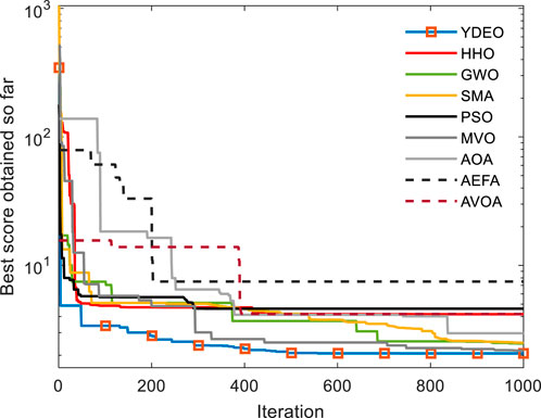
FIGURE A1. Convergence curve of YDEO when compared with other algorithms in the case of NedstackPS6 fuel cell.

FIGURE A2

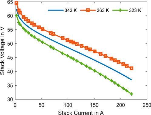
FIGURE A2. Polarization curves for different operating temperatures.

FIGURE A3

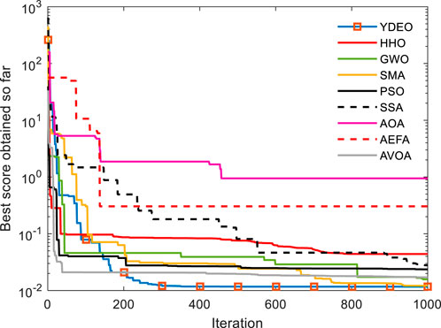
FIGURE A3. Convergence curve of YDEO when compared with other algorithms in the case of BCS500W fuel cell.

Nomenclature