AC/DC optimal power flow and techno-economic assessment for hybrid microgrids: TIGON CEDER demonstrator

In recent years, the interest in electric direct current (DC) technologies (such as converters, batteries, and electric vehicles) has increased due to their potential in energy efficiency and sustainability. However, the vast majority of electric systems and networks are based on alternating current (AC) as they also have certain advantages regarding cost-effective transport and robustness. In this paper, an AC/DC optimal power flow method for hybrid microgrids and several key performance indicators (KPIs) for its techno-economic assessment are presented. The combination of both calculations allows users to determine the viability of their hybrid microgrids. AC/DC networks have been modeled considering their most common elements. For the power flow method, polynomial optimization is formulated considering four different objective functions: the minimization of energy losses, voltage deviation, and operational costs and the maximization of the microgrid generation. The power flow method and the techno–economic analysis are implemented in Python and validated in the Centro de Desarrollo de Energías Renovables (CEDER) demonstrator for TIGON. The results show that the calculated power flow variables and those measured at CEDER are practically the same. In addition, the KPIs are obtained and compared for four operating scenarios: baseline, no battery, battery flexibility, and virtual battery (VB) flexibility. The last scenario results in the most profitable option.

1 Introduction

The global shift toward decarbonization has propelled significant transformations in the design, operation, and management of electric grids. The urgent need to mitigate climate change has led to the adoption of renewable energy sources and the phasing out of fossil fuel-based power generation, resulting in a paradigm shift in the electricity sector. The integration of variable renewable sources, such as solar and wind, presents unique challenges due to their intermittent nature and geographical distribution. As a result, electric grids have witnessed a remarkable transition toward more dynamic, flexible, and intelligent systems.

Microgrids (Lasseter, 2002; Hatziargyriou et al., 2007; Katiraei et al., 2008; Salam et al., 2008; Saeed et al., 2021) are localized and self-contained electricity distribution systems. They have gained prominence due to their ability to effectively integrate distributed energy resources (DERs). DERs include small-scale renewable energy installations, energy storage systems, and demand response capabilities. Microgrids provide an innovative solution to enhance the resilience, reliability, and sustainability of the electric grid at a smaller scale while offering opportunities for local energy generation, utilization, and management. In general, microgrids can work as an island or connected to the main power network, which acts as an external grid (Marnay et al., 2015).

Furthermore, the choice between alternating current (AC) and direct current (DC) elements within microgrids has become a subject of considerable interest (Wang et al., 2013). While AC has historically been the dominant standard for power transmission and distribution, recent advancements in DC technologies, such as state-of-the-art batteries and electric vehicles (EVs), have brought attention to these systems (Shao and Agelidis, 2010; Shi et al., 2017; Fotopoulou et al., 2021).

In microgrids, where local generation and consumption are tightly integrated, DC elements offer several benefits (Saeedifard et al., 2010; Rauf et al., 2016; Zubieta, 2016; Pires et al., 2023). First, DC distribution systems enable higher efficiency in the utilization of renewable energy sources. Most renewable energy technologies, such as solar panels and batteries, inherently generate and store DC power. By directly integrating these DC sources into the microgrid without the need for AC/DC conversions, energy losses associated with multiple conversions can be minimized, resulting in improved overall system efficiency. Moreover, DC systems offer increased flexibility for the integration of emerging technologies. As the demand for EVs grows, the DC charging infrastructure becomes crucial. DC microgrids can seamlessly accommodate EV charging stations without the need for additional power conversion equipment, reducing infrastructure costs and improving charging efficiency (Ashique et al., 2017).

Despite that, AC technologies still offer certain advantages that make them relevant and preferred in specific aspects of microgrid design and operation. For instance, high-voltage AC transmission systems inherently offer better voltage control than DC through reactive power, they are easier to isolate and interrupt in the case of faults, and the existing infrastructure is more abundant. In the end, both AC and DC technologies have their unique advantages and limitations, and their selection should be based on the careful evaluation and analysis of the specific circumstances. In this context, hybrid AC/DC microgrids emerge as a suitable solution for the transition to an electricity system with reduced or zero greenhouse gas emissions, taking advantage of the benefits of both forms of electricity current. One example of a project that seeks to maximize the benefits of these networks is the Horizon 2020 European project called Towards Intelligent DC-based hybrid Grids Optimizing the Network performance (TIGON). It also aims to improve the reliability, resilience, performance, and cost efficiency of hybrid AC/DC grids.

The main contribution of this article is the development of a procedure to study and evaluate the correct operation and the technical and economic feasibility of hybrid microgrid installations. The developed procedure consists of two components. The first component is a power flow calculation method for hybrid AC/DC microgrids based on optimization. The power flow can be performed by choosing among four different cost functions, depending on the objective to be achieved. The method is based on the recent literature on both AC and DC load flows (Agundis-Tinajero et al., 2018, 2019; Tinajero et al., 2021; Chopra et al., 2022) but differs from them by including a larger number of elements and a different formulation. The second component is a techno-economic evaluation based on key performance indicators (KPIs). In this case, several references were used (Sartori et al., 2014; Papapetrou et al., 2017; Abadie and Chamorro, 2019; Kiran, 2022) although the methodology of this article differs as it is specifically adapted to hybrid AC/DC microgrids. Another contribution of the article is the validation of the developed procedure in a real hybrid microgrid located in the facilities of the Centro de Desarrollo de Energías Renovables (CEDER), which is part of the EU-funded TIGON project dedicated to the demonstration of innovations in hybrid microgrids for greener, more resilient, and safer power grids. The measurable variables in the CEDER hybrid AC/DC microgrid have been compared with the values obtained in the power flow simulation for validation, demonstrating the accuracy and validity of the developed procedure.

The remainder of this article is organized as follows: Section 2 presents the optimal power flow formulation and the possible objective functions that can be used for optimization. Section 3 presents the KPIs used for the techno-economic assessment. Section 4 details the characteristics of the TIGON CEDER demonstrator. Section 5 presents the experimental and simulation results for different operating scenarios. The conclusion is given in Section 6. Finally, the microgrid model used for the AC/DC optimal power flow and the techno-economic analysis is detailed in Appendix A.

2 AC/DC optimal power flow

The AC/DC optimal power flow allows us to study the feasibility of the microgrid operation, self-consumption capability, load supply, and power losses.

2.1 Formulation

The nomenclature used in the formulation of the problem is detailed at the end of the paper. All electrical variables are represented in phasor form. Consider an electrical network whose topology is represented by a graph $\mathcal{G}=(\mathcal{B},\mathcal{L})$, where $\mathcal{B}=\{1,\dots ,n\}$ is the set of buses (vertices) and $\mathcal{L}\subset \mathcal{B}\times \mathcal{B}$ is the set of lines (edges). The lines are unordered pairs of buses $(i,k)$, where $i$ and $k$ are the pair of buses connected by the line.

A bus $k$ is adjacent to another bus $i$ if there is a line connecting them, i.e., if $(i,k)\in \mathcal{L}$. The set of buses adjacent to bus $i$ is denoted by ${\mathcal{A}}_i$ and is defined as follows:

${\mathcal{A}}_i=\left\{k\in \mathcal{B}\mid \left(i,k\right)\in \mathcal{L}\right\}.(1)$

The state of the network variables is physically related (Alexander and Sadiku, 2013). First, the apparent power at each bus $S_i$ is expressed using Equation 2, where $I_i^{*}$ is the complex conjugate of $I_i$.

$S_i=V_i\cdot I_i^{*}.(2)$

$I_i$ is an aggregation of currents, as stated in Equation 3.

$I_i={\displaystyle \sum _{k\in {\mathcal{A}}_i}}\left(I_{ik}+I_{ik0}\right).(3)$

Both $I_{ik}$ and $I_{ik0}$ can be calculated using Ohm’s law, as shown in Equations 4, 5, respectively.

$I_{ik}=y_{ik}\cdot \left(V_i-V_k\right),(4)$

$I_{ik0}=\frac{b_{ik}\cdot V_i}{2}.(5)$

Power flow equations are obtained combining all the previous expressions. In the case of AC buses, the resulting expressions are Equations 6–7 (Montes and Castro, 1995; Samperio, 2023).

$\begin{array}{ll}\hfill P_i& ={\displaystyle \sum _{k\in {\mathcal{A}}_i}}\left[c_{ik}\cdot \left(e_i^2+f_i^2-e_i\cdot e_k-f_i\cdot f_k\right)+s_{ik}\cdot \left(e_i\cdot f_k-e_k\cdot f_i\right)\right.\hfill \\ \hfill & \left.+P_{\mathit{conv,ik}}\right],\hfill \end{array}(6)$

$\begin{array}{ll}\hfill Q_i& ={\displaystyle \sum _{k\in {\mathcal{A}}_i}}\left[c_{ik}\cdot \left(e_i\cdot f_k-e_k\cdot f_i\right)+s_{ik}\cdot \left(-e_i^2-f_i^2+e_i\cdot e_k\right.\right.\hfill \\ \hfill & \left.\left.+f_i\cdot f_k\right)+b_{ik}\cdot \frac{-e_i^2-f_i^2}{2}\right].\hfill \end{array}(7)$

$P_{\mathit{conv,ik}}$, which is the power injected or transferred from converters, is added to the active power load flow equation. In the case of DC buses, the expressions are Equations 8, 9.

$P_i={\displaystyle \sum _{k\in {\mathcal{A}}_i}}\left[c_{ik}\cdot e_i\cdot \left(e_i-e_k\right)+P_{\mathit{conv,ik}}\right],(8)$

$Q_i=0.(9)$

In any case, $P_i$ and $Q_i$ are the sum of generation and demand (Equations 10, 11).

$P_i=P_{\mathit{gen,i}}+P_{\mathit{load,i}},(10)$

$Q_i=Q_{\mathit{gen,i}}+Q_{\mathit{load,i}}.(11)$

At all times, $P_{\mathit{gen,i}}$ and $Q_{\mathit{gen,i}}$ are limited to the nominal power and the minimum power of the generators (Equations 12, 13, respectively).

$P_{\mathit{gen,nom,i}}\ge P_{\mathit{gen,i}},\ge P_{\mathit{gen,min,i}},(12)$

$Q_{\mathit{gen,nom,i}}\ge Q_{\mathit{gen,i}}.\ge Q_{\mathit{gen,min,i}}.(13)$

If two buses are connected through a converter, the expression that describes the power exchange between them is given by Equation 14.

$P_{\mathit{conv,ik}}=\frac{P_{\mathit{conv,ki}}}{{\eta }_{ik}}.(14)$

The maximum and minimum voltage limits of buses are maintained, as shown in Equation 15.

$V_{\mathit{max,i}}^2\ge e_i^2+f_i^2\ge V_{\mathit{min,i}}^2.(15)$

When grid-forming mode is activated in a converter, the voltage at the output bus of the converter is set to its nominal value, as described in Equation 16.

$e_i^2+f_i^2=1.(16)$

When the converter is in grid-following mode, this restriction is not considered.

The total current that lines can transport is limited by Equation 17.

$\begin{array}{ll}\hfill I_{\mathit{max,ik}}^2& \ge {\left[c_{ik}\cdot \left(e_i-e_k\right)+s_{ik}\cdot \left(f_k-f_i\right)\right]}^2+\left[c_{ik}\cdot \left(f_i-f_k\right)\right.\hfill \\ \hfill & {\left.+s_{ik}\cdot \left(e_i-e_k\right)\right]}^2.\hfill \end{array}(17)$

Transformers cannot exceed their nominal power when operating, as shown in Equations 18, 19.

$\begin{array}{ll}\hfill S_{n,ik}^2& \ge \left\{{\left[c_{ik}\cdot \left(e_i-e_k\right)+s_{ik}\cdot \left(f_k-f_i\right)\right]}^2+\left[c_{ik}\cdot \left(f_i-f_k\right)\right.\right.\hfill \\ \hfill & \left.{\left.+s_{ik}\cdot \left(e_i-e_k\right)\right]}^2\right\}\cdot \left(e_i^2+f_i^2\right),\hfill \end{array}(18)$

$\begin{array}{ll}\hfill S_{n,ik}^2& \ge \left\{{\left[c_{ik}\cdot \left(e_i-e_k\right)+s_{ik}\cdot \left(f_k-f_i\right)\right]}^2+\left[c_{ik}\cdot \left(f_i-f_k\right)\right.\right.\hfill \\ \hfill & \left.{\left.+s_{ik}\cdot \left(e_i-e_k\right)\right]}^2\right\}\cdot \left(e_k^2+f_k^2\right).\hfill \end{array}(19)$

In the case of converters, this limitation is expressed using Equation 20.

$S_{n,ik}\ge P_{\mathit{conv,ik}}.(20)$

2.2 Optimization

Four different objective functions $h$ can be chosen for minimization in the AC/DC optimal power flow, depending on the objective to be achieved.

1. H1: Total active power generated. This function focuses on reducing energy losses (Equation 21).

$H1={\displaystyle \sum _{i\in \mathcal{B}}}{P}_{\mathit{gen,i}}.(21)$

2. H2: Bus voltage deviation from their nominal value. This function focuses on achieving grid stability (Equation 22).

$H2={\displaystyle \sum _{i\in \mathcal{B}}}{\left(e_i^2+f_i^2-1\right)}^2.(22)$

3. H3: Total amount of operational costs associated with each generator. This function focuses on achieving economic savings (Equation 23).

$H3={\displaystyle \sum _{i\in \mathcal{B}}}O{C}_i\cdot P_{\mathit{gen,i}}.(23)$

4. H4: Active power microgrid generation. This function focuses on making the highest possible use of the available generation resources in the microgrid (Equation 24). The objective function is set to be negative in order to calculate maximization.

$H4=-{\displaystyle \sum _{i\in \mathcal{B}}}{P}_{\mathit{gen,i}}.(24)$

The variables that are optimized when performing the power flow are $e_i$, $f_i$, $P_{\mathit{gen,i}}$, $Q_{\mathit{gen,i}}$, and $P_{\mathit{conv,ik}}$.

3 Techno-economic assessment

The techno-economic assessment presented in this paper consists of the calculation of eight KPIs. They allow the evaluation of a microgrid in terms of costs, energy generation, storage capabilities, and financial feasibility. Moreover, it provides critical insights for making informed decisions and maximizing the overall performance of the microgrid. The KPIs, presented below, are divided into two categories: technical and economic.

3.1 Technical KPIs

$•$ KPI1: Electrical energy generated. This indicator represents the amount of electrical energy generated per year.

$KPI1\left(kWh\right)={\displaystyle \sum _{i\in \mathcal{B}}}{P}_{\mathit{gen,nom,i}}\cdot C{F}_i\cdot 8760.(25)$

$•$ KPI2: CO₂ emissions. This indicator represents the total CO₂ emitted by all energy carriers associated with the primary energy use in the microgrid per year.

$KPI2\left(kgC{O}_2\right)={\displaystyle \sum _{i\in \mathcal{B}}}{P}_{\mathit{gen,nom,i}}\cdot C{F}_i\cdot 8760\cdot GH{G}_i.(26)$

$•$ KPI3: Self-consumption percentage. This indicator represents the amount of energy obtained from the generators of the microgrid in relation to the energy used by the loads.

$KPI3\left(\%\right)=\frac{{\sum }_{i\in \mathcal{B}}{P}_{\mathit{gen,nom,i}}\cdot C{F}_i}{{\sum }_{i\in \mathcal{B}}{P}_{\mathit{load,i}}}.(27)$

$•$ KPI4: Storage flexibility. This indicator represents the total flexible power available in the microgrid due to the storage systems.

$KPI4\left(kW\right)={\displaystyle \sum _{i\in \mathcal{B}}}{P}_{\mathit{stor,i}}.(28)$

3.2 Economic KPIs

$•$ KPI5: Total life cycle income. This indicator represents the total income earned by the microgrid over its useful life. This index includes income from energy production and flexibility management.

$KPI5\left(currency\right)={\displaystyle \sum _{n=1}^{UL}}\frac{{\sum }_{i\in \mathcal{B}}\left(P_{\mathit{gen,nom,i}}\cdot C{F}_i\cdot EP\right)+FI}{{\left(1+r\right)}^n}.(29)$

$•$ KPI6: Total life cycle cost. This indicator represents the total cost incurred by the microgrid over its useful life. The index includes the investment, operation, and management costs and residual values of the microgrid and generators.

$\begin{array}{ll}\hfill KPI6\left(currency\right)& =IC+{\displaystyle \sum _{i\in \mathcal{B}}}\left(I{C}_i+O{C}_i\right)\hfill \\ \hfill & +{\displaystyle \sum _{n=1}^{UL}}\frac{OMC+{\displaystyle \sum _{i\in \mathcal{B}}}M{C}_i}{{\left(1+r\right)}^n}\hfill \\ \hfill & -\frac{RV-{\sum }_{i\in \mathcal{B}}R{V}_i}{{\left(1+r\right)}^{UL}}.\hfill \end{array}(30)$

$•$ KPI7: Payback. This indicator represents the period of time required to recover the capital investment of the microgrid (Kiran, 2022).

$\begin{array}{ll}\hfill KPI7\left(years\right)& =Nwhen\left({\displaystyle \sum _{n=1}^N}\frac{\left({\sum }_{i\in \mathcal{B}}{P}_{\mathit{gen,nom,i}}\cdot C{F}_i\cdot EP\right)+FI}{{\left(1+r\right)}^n}\right.\hfill \\ \hfill & =IC+{\displaystyle \sum _{i\in \mathcal{B}}}\left(I{C}_i+O{C}_i\right)\hfill \\ \hfill & \left.+{\displaystyle \sum _{n=1}^{UL}}\frac{OMC+{\displaystyle \sum _{i\in \mathcal{B}}}M{C}_i}{{\left(1+r\right)}^n}-\frac{RV-{\sum }_{i\in \mathcal{B}}R{V}_i}{{\left(1+r\right)}^{UL}}\right).\hfill \end{array}(31)$

$•$ KPI8: Levelized cost of energy (LCOE). This indicator represents the price at which the generated electricity should be sold to break even by the end of the useful life of the microgrid (Papapetrou et al., 2017; Abadie and Chamorro, 2019).

$\begin{array}{l}\hfill KPI8\left(currency/kWh\right)=\\ \hfill & \frac{IC+{\displaystyle \sum _{i\in \mathcal{B}}}\left(I{C}_i+O{C}_i\right)+{\displaystyle \sum _{n=1}^{UL}}\frac{OMC+{\displaystyle \sum _{i\in \mathcal{B}}}M{C}_i}{{\left(1+r\right)}^n}-\frac{RV-{\sum }_{i\in \mathcal{B}}R{V}_i}{{\left(1+r\right)}^{UL}}}{{\displaystyle \sum _{n=1}^{UL}}\frac{{\sum }_{i\in \mathcal{B}}{P}_{\mathit{gen,nom,i}}\cdot C{F}_i}{{\left(1+r\right)}^n}}.\hfill \end{array}(32)$

4 TIGON CEDER demonstrator

CEDER is the acronym for Center for the Development of Renewable Energies¹. It is located in Lubia (Soria, Spain) and serves as a national center for energy research that belongs to the Center for Energy, Environmental, and Technological Research (CIEMAT)², a public research organization under the Ministry of Science and Innovation. This facility covers an area of 640 ha (13,000 m² built) and features a smart microgrid (electrical and thermal) operated and managed in real time (see Figure 1, left).

Figure 1

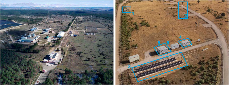
Figure 1. CEDER facilities (left) and TIGON demonstrator (right).

The Spanish demonstrator of TIGON is installed at CEDER (see Figure 1, right) and consists of the following elements:

1. Transformer station: 15 kV_AC–400 V_AC.

2. Small wind turbine: A three-bladed, horizontal axis wind turbine with a nominal power of 4.2 kW (Ryse E-5).

3. Photovoltaic (PV) system: Comprising 3 strings with 18 modules (URECO) of 410 W each, amounting to a total capacity of 22.14 kW.

4. NMC batteries: 3 modules, each with 80 cells (50 Ah and 3.6 V per cell).

5. Programmable AC loads: Three programmable AC loads of 2.9 kW each.

6. DC loads: Three adjustable DC loads of 4 kW each.

A schematic diagram of the CEDER demonstrator is shown in Figure 2. It consists of AC loads, wind turbines, transformers, and DC sections in the network. The characteristics of the elements used to test the microgrid are given in Tables 1–3.

Figure 2

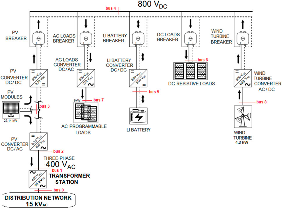
Figure 2. TIGON layout at CEDER.

Table 1

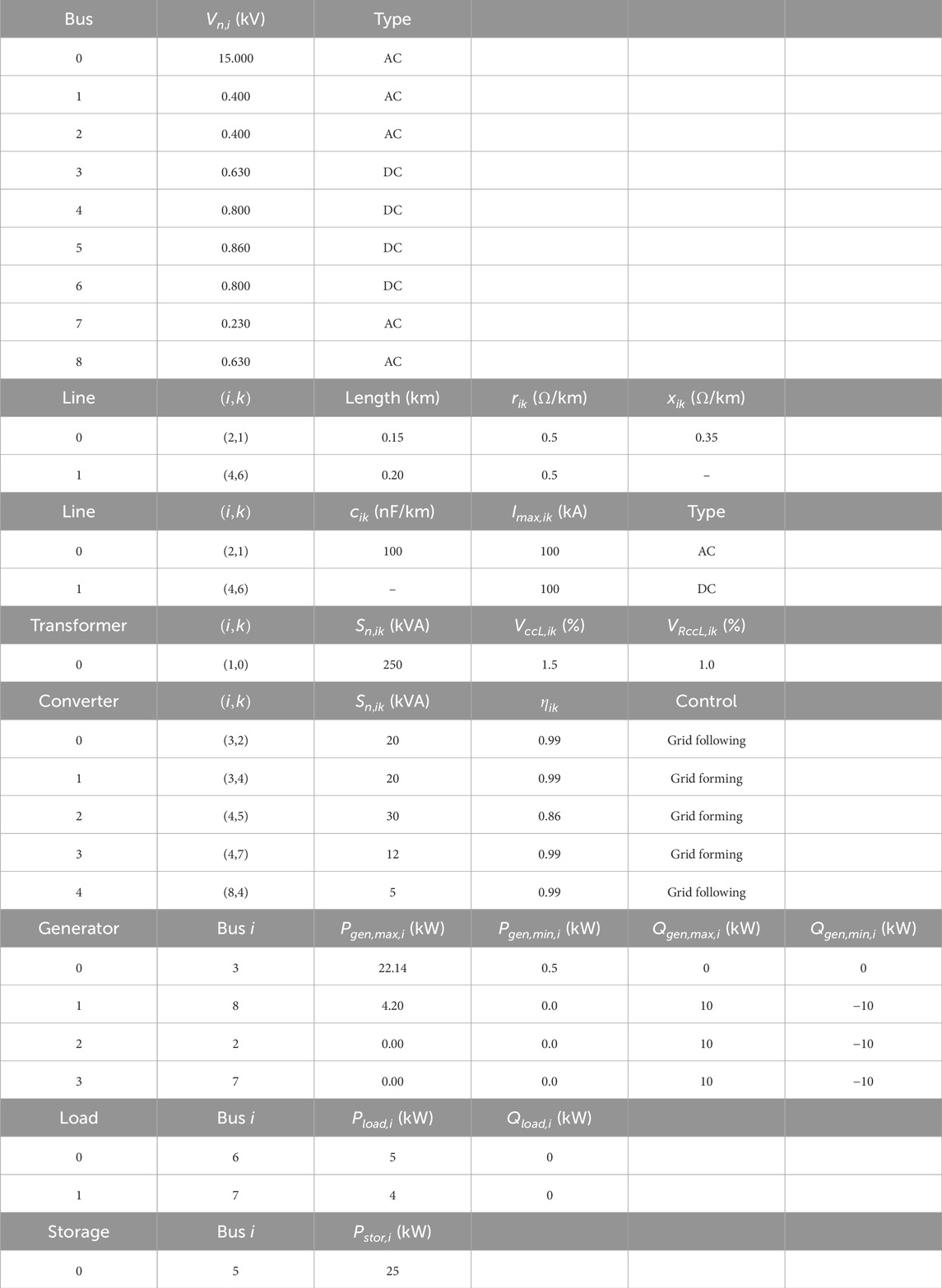
Table 1. TIGON CEDER electrical data.

Table 2

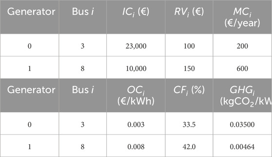
Table 2. Techno-economic information of TIGON CEDER generators.

Table 3

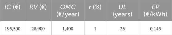
Table 3. Techno–economic information of the TIGON CEDER microgrid.

$V_{\mathit{max,i}}$ and $V_{\mathit{min,i}}$ have been fixed at 5% above and below the nominal value, respectively. $GH{G}_i$ of generators 0 and 1 have been obtained from the study by Baldwin (2006). Generators 2 and 3 model the reactive power management of converters 0 and 3, respectively. The CEDER microgrid has one connection to an external grid located on bus 0. The frequency is 50 Hz ($\omega =100\pi$ rad/s).

$IC$ and $RV$ have been calculated as the sum of the investment cost and the residual value of the microgrid equipment and labor, as given in Table 4.

Table 4

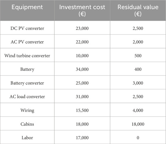
Table 4. Investment costs and residual values of TIGON CEDER equipment and labor.

5 Results and discussion

5.1 AC/DC optimal power flow

The AC/DC optimal power flow simulation has been implemented in Python due to its wide range of available open-source optimization libraries. In this paper, the optimization has been performed using CasADi (Andersson et al., 2019), which is a software library equipped with specific tools focused on the modeling, optimization, and control of nonlinear dynamic systems. CasADi is widely used to define both mathematical models and constraints involved and allows us to utilize different solvers in order to optimize the problem. In this study, the solver IPOPT (Wächter and Biegler, 2006) has been used. IPOPT applies sequential quadratic programming (SQP) to solve constrained nonlinear optimization problems, which is the case in the AC/DC optimal power flow. The calculation time is not significant: it is only a few seconds.

Four scenarios have been tested, one per objective function. In all scenarios, TIGON CEDER storage has been considered to act as a load that consumes electricity at half its nominal power ($P_{\mathit{stor}}$/2), and the external grid has been limited to power consumption (if required). The results obtained in each scenario are given in Table 5.

Table 5

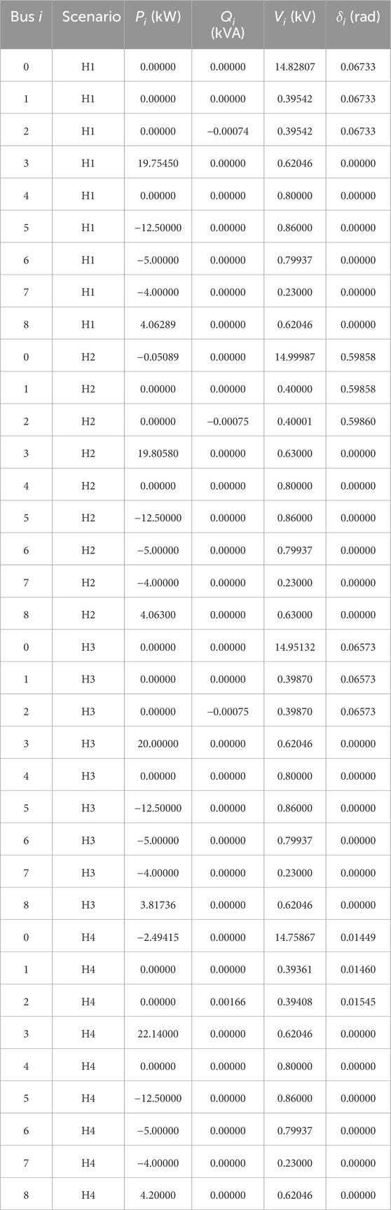
Table 5. Simulation results for different scenarios.

In all scenarios, all the power demanded by loads and storage is delivered. In none of them exists the demand for reactive power, so all the reactive power in the microgrid is generated in the AC section at bus 2 because of the transformer and AC line reactance.

In scenarios H1 and H3, the exact active power is generated to supply the demand and compensate for losses. The difference between them is that the wind turbine reduces its active power generation in scenario H3 because this technology has higher operational costs than the PV, whereas more power is saved in scenario H1.

In scenario H2, $V_i$ at all buses is the nominal value or very close to it. To achieve it, the generation of active power and the consumption of the external grid are precisely adjusted.

In scenario H4, the PV and wind turbine generate the maximum active power, which is then supplied to the external grid.

All the scenarios have been recreated in the real environment of the TIGON CEDER microgrid. The two quantities accessed for measurement are active power and voltage. The values obtained in the measurements taken for each scenario are shown in Table 6.

Table 6

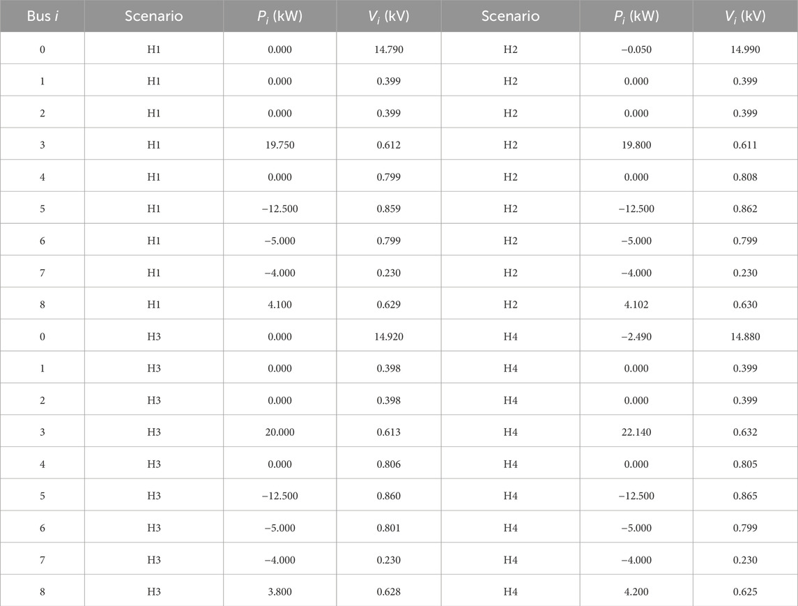
Table 6. CEDER microgrid measurements for different scenarios.

The measures obtained are very similar to the calculated values in the simulations, as shown in Figures 3, 4. In Table 7, the mean relative error (MRE) has been calculated for both active power and voltage using Equation Equation 33.

$MRE\left(\%\right)=\frac{100}{N}\cdot {\displaystyle \sum _{i=0}^{N-1}}\frac{|{\widehat{a}}_i-a_i|}{|a_i|}.(33)$

Figure 3

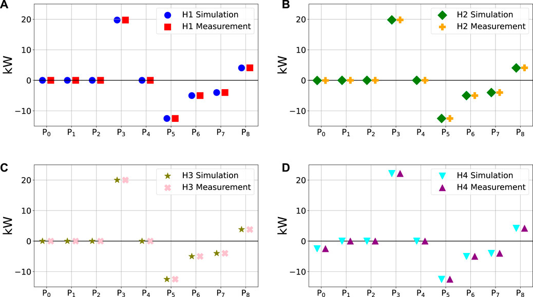
Figure 3. Comparison of simulation and measurement values of active power: (A) scenario H1, (B) scenario H2, (C) scenario H3, and (D) scenario H4.

Figure 4

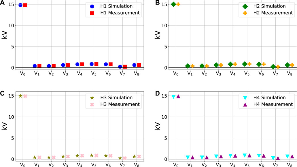
Figure 4. Comparison of simulation and measurement values of voltage: (A) scenario H1, (B) scenario H2, (C) scenario H3, and (D) scenario H4.

Table 7

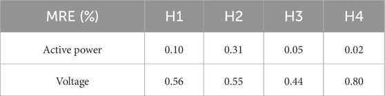
Table 7. Mean relative error of measurements.

The largest differences are observed between the expected and actually measured PV voltages, with a maximum relative error of 3.11%. This occurs because the PV voltage (bus 3) varies considerably as the delivered active power changes. Small differences in accuracy arise from the monitoring devices and the difficulty of precisely obtaining at the same time the proposed values of active power generation from both the wind turbine and PV due to their inherent variability depending on the weather conditions and technical restrictions.

The results confirm that the AC/DC optimal power flow works correctly and accurately enough to assess the operation of the microgrid.

5.2 Techno-economic assessment

The techno-economic assessment calculations have been implemented in Python. Again, the calculation time is very short, only a few seconds. Four scenarios in which the TIGON CEDER microgrid could operate have been studied: baseline, no battery, battery flexibility, and virtual battery (VB) flexibility.

In the baseline scenario, the microgrid elements have been considered with the same characteristics presented in Section 4. Nevertheless, in this situation, which is real, the battery is being used only for performing tests and research experiments. For this reason, we have considered three more scenarios in which the microgrid could be more profitable. In the no-battery scenario, the battery and its converter have been removed from the microgrid, along with their investment costs and residual values. In the battery flexibility scenario, the battery has not been eliminated, but it has been deemed to be used in the Spanish upward tertiary regulation market. Batteries are loads with inherent electrical flexibility as they can be charged and discharged at the most convenient time, keeping the daily balance of the generated and consumed electricity unchanged. The upward tertiary regulation market has been chosen because it is the balance market with the highest average price in Spain in 2022: 224.17 €/MWh³. The power of the battery is very small to participate in the Spanish tertiary regulation market on its own as it is necessary to make bids of at least 1 MW (Red Eléctrica de España, 2021). Therefore, it needs to be part of an aggregation that participates in the market as a unitary market agent, following the methodology explained by Martín-Crespo et al. (2023). Lastly, in the VB flexibility scenario, the battery has been replaced by a VB consisting of an aggregation of thermostatically controlled loads (TCLs) already in place, with the same nominal power $P_{\mathit{stor,i}}$. These TCLs have the capacity to store thermal energy equivalent to a given electricity consumption. They could be heat pumps or water heaters, for instance. The aggregation of TCLs in the VB has been achieved using the method proposed by Martín-Crespo et al. (2021). This method is a control algorithm executed in real time and consists of three steps: Check of TCLs, Aggregation, and Priority Control. As a result of these stages, the controller decides which TCLs should be switched on or off to meet the stated power requirement. For both flexibility scenarios, storage participation in the market for 1 h per day is assumed to operate at its nominal power $P_{\mathit{stor,i}}$ and the aggregation shares its benefits proportionally between its loads. This results in an additional flexibility income $FI$ of 2,045.55 € per year.

The KPI values obtained for each scenario are given in Table 8.

Table 8

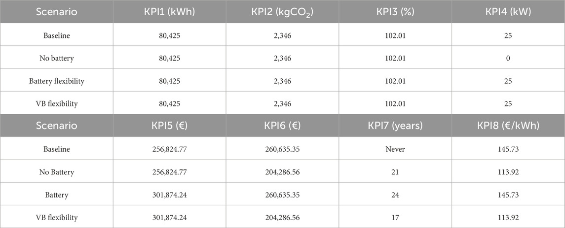
Table 8. KPI results.

KPI2 (CO₂) proves that carbon dioxide emissions are very low. This is caused by the usage of renewable generation technologies, specifically PV and wind turbines. KPI3 (self-consumption percentage) shows that the microgrid produces more energy than required by the loads per year, thus compensating for energy losses.

KPI7 (payback) shows that in the baseline scenario, the microgrid is not profitable. It makes sense as the TIGON CEDER microgrid is a small-scale network where the elements are high-cost prototypes. The battery, which is the storage element of the grid, is key for increasing or decreasing costs and incomes. The battery flexibility scenario demonstrates that using the battery for making bids in the Spanish electricity balance markets enhances the incomes and makes the microgrid profitable. Nevertheless, the flexibility remuneration is not high enough to make the microgrid payback lower than that when the battery is removed, i.e., the no-battery scenario. In the no-battery scenario, costs are highly reduced, as well as in KPI8 (LCOE). This is at the expense of reducing KPI4 (storage flexibility) to zero. The most profitable scenario is VB flexibility as it combines the additional income obtained by participation in the tertiary regulation market with the cost savings caused by the disappearance of the physical battery. KPI7 (payback) is reduced to 17 years and KPI8 (LCOE) to 113.92 €/kWh, whereas KPI4 (storage flexibility) remains at 25 kW.

6 Conclusion

In this paper, an AC/DC optimal power flow and a techno-economic assessment have been presented with the aim of helping users evaluate the operation and viability of their hybrid AC/DC microgrids. In addition, both calculations can be used for proposing improvements and new investments. The AC/DC optimal power flow is a useful technique for checking the correct operation of hybrid microgrids under specific instantaneous conditions, while the techno-economic assessment allows us to verify their performance in the long term.

Both methodologies have been tested on the TIGON CEDER microgrid, which has been described in this paper. The AC/DC optimal power flow has been validated using real measurements and considering different objective function scenarios. Among the four techno-economic scenarios, the VB flexibility scenario is the most profitable and offers the fastest return on investment. Based on the results of flexibility scenarios, we encourage the stakeholders in the Spanish electricity system to increase the remuneration of flexibility to increase the penetration of renewable energy sources and advance the transition to a more efficient AC/DC hybrid power system with low greenhouse gas emissions.

In future work, we will apply the AC/DC optimal power flow and the techno-economic assessment to other microgrids, especially those primarily aimed at supplying electricity to residential consumers and industries. We also hope that the two developed techniques and the TIGON CEDER microgrid example can be used by other companies and research institutions in their developments.

Data availability statement

The raw data supporting the conclusion of this article will be made available by the authors, without undue reservation.

Author contributions

AM-C: conceptualization, data curation, formal analysis, investigation, methodology, software, validation, visualization, writing–original draft, and writing–review and editing. AH-S: conceptualization, formal analysis, investigation, methodology, project administration, software, and writing–review and editing. ÓI-M: conceptualization, data curation, formal analysis, investigation, project administration, resources, validation, visualization, and writing–review and editing. PP-C: investigation, resources, and writing–review and editing. ÁH-J: investigation, resources, and writing–review and editing. FF-E: conceptualization, methodology, supervision, and writing–review and editing. EB: conceptualization, methodology, supervision, and writing–review and editing.

Funding

The author(s) declare that financial support was received for the research, authorship, and/or publication of this article. This research received funding from the European Union’s Horizon 2020 TIGON project under grant agreement no. 957769.

Conflict of interest

The authors declare that the research was conducted in the absence of any commercial or financial relationships that could be construed as a potential conflict of interest.

Publisher’s note

All claims expressed in this article are solely those of the authors and do not necessarily represent those of their affiliated organizations, or those of the publisher, the editors, and the reviewers. Any product that may be evaluated in this article, or claim that may be made by its manufacturer, is not guaranteed or endorsed by the publisher.

Footnotes

¹http://www.ceder.es/

²https://www.ciemat.es/portal.do?IDM=6&NM=1

³https://www.sistemaelectrico-ree.es/informe-del-sistema-electrico/mercados/servicios-ajuste/energias-precios-balance

References

Abadie, L., and Chamorro, J. (2019). Levelized cost of electricity: key drivers and valuation methods. Dyna 94, 656–661. doi:10.6036/9223

CrossRef Full Text | Google Scholar

Agundis-Tinajero, G., Aldana, N. L. D., Luna, A. C., Segundo-Ramírez, J., Visairo-Cruz, N., Guerrero, J. M., et al. (2018). Extended-optimal-power-flow-based hierarchical control for islanded ac microgrids. IEEE Trans. Power Electron. 34, 840–848. doi:10.1109/tpel.2018.2813980

CrossRef Full Text | Google Scholar

Agundis-Tinajero, G., Segundo-Ramírez, J., Visairo-Cruz, N., Savaghebi, M., Guerrero, J. M., and Barocio, E. (2019). Power flow modeling of islanded ac microgrids with hierarchical control. Int. J. Electr. Power and Energy Syst. 105, 28–36. doi:10.1016/j.ijepes.2018.08.002

CrossRef Full Text | Google Scholar

Alexander, C. K., and Sadiku, M. N. (2013). Fundamentos de circuitos elétricos. McGraw-Hill Interamericana de España S.L.

Google Scholar

Andersson, J. A. E., Gillis, J., Horn, G., Rawlings, J. B., and Diehl, M. (2019). CasADi – a software framework for nonlinear optimization and optimal control. Math. Program. Comput. 11, 1–36. doi:10.1007/s12532-018-0139-41007/s12532-018-0139-4

CrossRef Full Text | Google Scholar

Ashique, R. H., Salam, Z., Aziz, M. J. B. A., and Bhatti, A. R. (2017). Integrated photovoltaic-grid dc fast charging system for electric vehicle: a review of the architecture and control. Renew. Sustain. Energy Rev. 69, 1243–1257. doi:10.1016/j.rser.2016.11.245

CrossRef Full Text | Google Scholar

Baldwin, S. (2006). Carbon footprint of electricity generation. Parliam. Office Sci. Technol. 268.

Google Scholar

Chopra, S., Vanaprasad, G. M., Tinajero, G. D. A., Bazmohammadi, N., Vasquez, J. C., and Guerrero, J. M. (2022). Power-flow-based energy management of hierarchically controlled islanded ac microgrids. Int. J. Electr. Power and Energy Syst. 141, 108140. doi:10.1016/j.ijepes.2022.108140

CrossRef Full Text | Google Scholar

Cui, Y. (2017). “Static parameter detection and identification of power grid branch based on PMU measurement,” in 2016 4th international conference on machinery, materials and information technology applications (Atlantis Press), 313–318.

Google Scholar

Fotopoulou, M., Rakopoulos, D., Trigkas, D., Stergiopoulos, F., Blanas, O., and Voutetakis, S. (2021). State of the art of low and medium voltage direct current (DC) microgrids. Energies 14, 5595. doi:10.3390/en14185595

CrossRef Full Text | Google Scholar

Hatziargyriou, N., Asano, H., Iravani, R., and Marnay, C. (2007). Microgrids. IEEE power energy Mag. 5, 78–94. doi:10.1109/mpae.2007.376583

CrossRef Full Text | Google Scholar

Katiraei, F., Iravani, R., Hatziargyriou, N., and Dimeas, A. (2008). Microgrids management. IEEE power energy Mag. 6, 54–65. doi:10.1109/mpe.2008.918702

CrossRef Full Text | Google Scholar

Kiran, D. (2022). Principles of economics and management for manufacturing engineering. Butterworth-Heinemann.

Google Scholar

Lasseter, R. H. (2002). “Microgrids,” in 2002 IEEE power engineering society winter meeting. Conference proceedings (Cat. No. 02CH37309) (IEEE), 1, 305–308. doi:10.1109/pesw.2002.985003

CrossRef Full Text | Google Scholar

Marnay, C., Chatzivasileiadis, S., Abbey, C., Iravani, R., Joos, G., Lombardi, P., et al. (2015). “Microgrid evolution roadmap,” in 2015 international symposium on smart electric distribution systems and technologies (EDST) (IEEE), 139–144.

CrossRef Full Text | Google Scholar

Martín-Crespo, A., Baeyens, E., Saludes-Rodil, S., and Frechoso-Escudero, F. (2023). Aggregated demand flexibility prediction of residential thermostatically controlled loads and participation in electricity balance markets. arXiv preprint arXiv:2308.04853.

Google Scholar

Martín-Crespo, A., Saludes-Rodil, S., and Baeyens, E. (2021). Flexibility management with virtual batteries of thermostatically controlled loads: real-time control system and potential in Spain. Energies 14, 1711. doi:10.3390/en14061711

CrossRef Full Text | Google Scholar

Mohammed, S. A. Q., and Jung, J.-W. (2021). A state-of-the-art review on soft-switching techniques for DC–DC, DC–AC, AC–DC, and AC–AC power converters. IEEE Trans. Industrial Inf. 17, 6569–6582. doi:10.1109/tii.2021.3058218

CrossRef Full Text | Google Scholar

Montes, A., and Castro, J. (1995). Solving the load flow problem using gröbner basis. ACM SIGSAM Bull. 29, 1–13. doi:10.1145/216685.216686

CrossRef Full Text | Google Scholar

Papapetrou, M., Cipollina, A., La Commare, U., Micale, G., Zaragoza, G., and Kosmadakis, G. (2017). Assessment of methodologies and data used to calculate desalination costs. Desalination 419, 8–19. doi:10.1016/j.desal.2017.05.038

CrossRef Full Text | Google Scholar

Pires, V. F., Pires, A., and Cordeiro, A. (2023). DC microgrids: benefits, architectures, perspectives and challenges. Energies 16, 1217. doi:10.3390/en16031217

CrossRef Full Text | Google Scholar

Quezada, V. M., Abbad, J. R., and Roman, T. G. S. (2006). Assessment of energy distribution losses for increasing penetration of distributed generation. IEEE Trans. power Syst. 21, 533–540. doi:10.1109/tpwrs.2006.873115

CrossRef Full Text | Google Scholar

Rauf, S., Wahab, A., Rizwan, M., Rasool, S., and Khan, N. (2016). Application of dc-grid for efficient use of solar PV system in smart grid. Procedia Comput. Sci. 83, 902–906. doi:10.1016/j.procs.2016.04.182

CrossRef Full Text | Google Scholar

Red Eléctrica de España (2021). Guía descriptiva. Ser Proveed. Serv. balance. Versión 03. (in Spanish).

Google Scholar

Saeed, M. H., Fangzong, W., Kalwar, B. A., and Iqbal, S. (2021). A review on microgrids’ challenges and perspectives. IEEE Access 9, 166502–166517. doi:10.1109/access.2021.3135083

CrossRef Full Text | Google Scholar

Saeedifard, M., Graovac, M., Dias, R., and Iravani, R. (2010). “DC power systems: challenges and opportunities,” in IEEE PES general meeting (IEEE), 1–7.

CrossRef Full Text | Google Scholar

Salam, A., Mohamed, A., and Hannan, M. (2008). Technical challenges on microgrids. ARPN J. Eng. Appl. Sci. 3, 64–69.

Google Scholar

Samperio, Á. (2023). Sparse recovery of an electrical network. arXiv preprint arXiv:2304.06676.

Google Scholar

Sartori, D., Catalano, G., Genco, M., Pancotti, C., Sirtori, E., Vignetti, S., et al. (2014). Guide to cost-benefit analysis of investment projects. Economic appraisal tool for cohesion policy 2014-2020, European Commission. Directorate-General for Regional and Urban policy. Tech. Rep.

Google Scholar

Shao, S. J., and Agelidis, V. G. (2010). Review of DC system technologies for large scale integration of wind energy systems with electricity grids. Energies 3, 1303–1319. doi:10.3390/en3061303

CrossRef Full Text | Google Scholar

Shi, R., Semsar, S., and Lehn, P. W. (2017). Constant current fast charging of electric vehicles via a DC grid using a dual-inverter drive. IEEE Trans. Industrial Electron. 64, 6940–6949. doi:10.1109/tie.2017.2686362

CrossRef Full Text | Google Scholar

Tinajero, G. D. A., Nasir, M., Vasquez, J. C., and Guerrero, J. M. (2021). Comprehensive power flow modelling of hierarchically controlled AC/DC hybrid islanded microgrids. Int. J. Electr. Power and Energy Syst. 127, 106629. doi:10.1016/j.ijepes.2020.106629

CrossRef Full Text | Google Scholar

Wächter, A., and Biegler, L. T. (2006). On the implementation of an interior-point filter line-search algorithm for large-scale nonlinear programming. Math. Program. 106, 25–57. doi:10.1007/s10107-004-0559-y

CrossRef Full Text | Google Scholar

Wang, P., Goel, L., Liu, X., and Choo, F. H. (2013). Harmonizing AC and DC: a hybrid AC/DC future grid solution. IEEE Power Energy Mag. 11, 76–83. doi:10.1109/mpe.2013.2245587

CrossRef Full Text | Google Scholar

Zubieta, L. E. (2016). Are microgrids the future of energy? DC microgrids from concept to demonstration to deployment. IEEE Electrification Mag. 4, 37–44. doi:10.1109/mele.2016.2544238

CrossRef Full Text | Google Scholar

Appendix A

Microgrid Model

The $\pi$ model representation of grid lines (Figure A1 (Cui, 2017; Alexander and Sadiku, 2013)) is used for performing the AC/DC optimal power flow. In the case of DC lines, $s_{ik}$ and $b_{ik}$ are not considered, as the reactive part of impedances does not affect electric charges when they move always in the same direction over time.

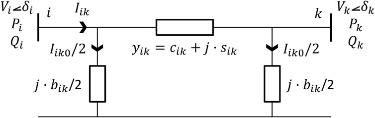
FIGURE A1

FIGURE A1. $\pi$ model of lines.

$y_{ik}$ is the inverse of the line impedance $z_{ik}$, which is expressed by Equation A1.

$z_{ik}=r_{ik}+j\cdot x_{ik}.(\mathrm{A1})$

Both $r_{ik}$ and $x_{ik}$ are directly proportional to the line length, and, in the case of $x_{ik}$, also the frequency. In the case of DC lines, $x_{ik}$ is not considered because it is a reactive parameter. For AC cases, $b_{ik}$ is obtained using Equation A2.

$b_{ik}=\omega \cdot C_{ik}.(\mathrm{A2})$

$C_{ik}$ is directly proportional to the line length. Each line has a current limit $I_{\mathit{max,ik}}$.

Voltage at each bus can be expressed by its real and imaginary part, as in Equation A3

$V_i=e_i+j\cdot f_i.(\mathrm{A3})$

The bus voltage phase ${\delta }_i$ can be calculated by Equation A4.

${\delta }_i=\arctan \frac{f_i}{e_i}.(\mathrm{A4})$

Each bus of the grid can have a different reference voltage. In order to ease load flow calculations in grids where voltage and current transformations occur through converters or transformers, a base power $S_{\mathit{base}}$ and a base voltage $V_{\mathit{base}}$ are set. Base impedance $z_{\mathit{base}}$ is calculated as in Equation A5.

$z_{\mathit{base}}=\frac{V_{\mathit{base}}^2}{S_{\mathit{base}}}.(\mathrm{A5})$

All magnitudes in the grid model are divided by their base values, so they can be expressed per unit (p.u.). Maximum and minimum voltages at each bus are specified ($V_{\mathit{max}}$ and $V_{\mathit{min}}$, respectively).

Transformers in the grid are modelled in the same way as lines, but without taking $b_{ik}$ into account because it is considered to have a minimal impact on the total transformer impedance. The magnitude and the resistive part of their $z_{ik}$ are calculated with Equations A6, A7.

$|z_{ik}|=\frac{V_{\mathit{ccL,ik}}\cdot V_{LN,ik}^2}{100\cdot S_{n,ik}},(\mathrm{A6})$

$r_{ik}=\frac{V_{\mathit{RccL,ik}}\cdot V_{LN,ik}^2}{100\cdot S_{n,ik}}.(\mathrm{A7})$

Besides transformers, converters are the other grid elements that changes voltage levels between buses. There exists AC/DC, DC/AC, AC/AC and DC/DC converters (Mohammed and Jung, 2021). Their characteristics needed to perform load flow calculations are nominal power $S_{n,ik}$, performance ${\eta }_{ik}$ and control mode (grid-following or grid-forming). The reactive power at the output of DC/AC and AC/AC converters is included in the grid model of this paper as a reactive power generator in order to recreate the reactive power management operation of these converters.

All generators existing in the microgrid are characterized by their nominal active power $P_{\mathit{gen,nom,i}}$, minimum active power $P_{\mathit{gen,min,i}}$, nominal reactive power $Q_{\mathit{gen,nom,i}}$ and minimum reactive power $Q_{\mathit{gen,min,i}}$. Regarding loads, they are defined by two parameters: demanded active power $P_{\mathit{load,i}}$ and demanded reactive power $Q_{\mathit{load,i}}$. Supplying $P_{\mathit{load,i}}$ and $Q_{\mathit{load,i}}$ is considered mandatory. In the case of storages, they can act as generators of loads in the power flow. Their defining parameter is $P_{\mathit{stor,i}}$.

If present, external grids are considered to be capable of providing and consuming active power and reactive power with no limits, but not at the same time.

For the techno-economic assessment, additional information about generators is considered. This includes their investment cost $I{C}_i$, residual value $R{V}_i$, maintenance cost $M{C}_i$, operational cost $O{C}_i$, capacity factor $C{F}_i$ and CO₂ equivalent $GH{G}_i$. $C{F}_i$ is the percentage of power produced by the generator with respect to the power that could have been produced if the generator had operated at maximum rate (Quezada et al., 2006).

Regarding the rest of the microgrid, investment cost $IC$, residual value $RV$, operation and maintenance cost $OMC$ and useful life $UL$ are used. In addition, the price at which the microgrid sells electricity $EP$,and the discount rate $r$ are included in the model. Flexibility income $FI$ is considered in the flexibility scenario of the techno-economic analysis.

Nomenclature