 Qiufen Sun1
 Maohan Yuan
- 1PetroChina Hangzhou Research Institute of Geology, Hangzhou, China
- 2School of Petroleum and Natural Gas Engineering, Southwest Petroleum University, Chengdu, China
It has been widely accepted that China is one of the biggest natural gas consumers. Related to the imports of LNG, China stands in a very uncomfortable situation. Most domestic gas reservoirs fall within deep water drive gas reservoirs inordinately, which has entered the production depletion stage. Accurate estimation of SEC recoverable reserves of deep water drive gas reservoirs is of great significance for gas consumption planning and peak shaving. The existing calculation methods of recoverable reserves mainly consist of static methods and dynamic methods. In the early stage of exploration and development, the volumetric method has often been utilized to calculate the recoverable reserves. With the continuous development of gas reservoirs, the main methods for evaluation are dynamic methods, including the successive subtraction of production method, water drive curve method, prediction model method, attenuation curve method, improved virtual curve method, and material balance method for deep gas reservoirs.
1 Introduction
Since the beginning of the 21st century, the natural gas industry in China has witnessed remarkable growth, as shown in Figure 1: the domestic natural gas output has increased rapidly from 274 × 108 m3 in 2000 to 2,201.1 × 108 m3 in 2022. Additionally, the proportion of natural gas in the total primary energy production has increased significantly, increasing from 2.6% in 2000 to 5.9% in 2022 (Statistics, 2023). With the proposal of the dual carbon goal, natural gas is increasingly being recognized as a clean and low-carbon fuel source.
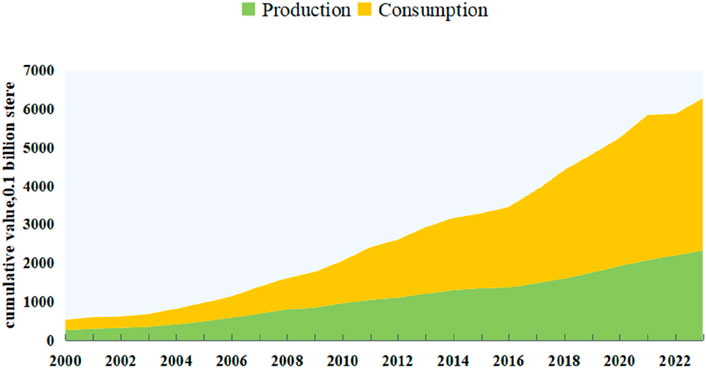
Figure 1. NG production and consumption in China from 2000 to 2024.
China boasts rich natural gas resources. To ensure national energy security and achieve the dual objectives of economic development and environmental protection, the government has been committed to vigorously enhancing domestic oil and gas exploration and development. Natural gas exploration and development has broadened its scope, moving beyond structural gas reservoirs to lithologic gas reservoirs and covering a range of different types of gas reservoirs, including single carbonate gas reservoirs, loose sandstone gas reservoirs, low-permeability tight gas reservoirs, volcanic gas reservoirs, shale gas, coal bed gas, and others (Xie et al., 2018). The depth of gas reservoirs has also expanded, ranging from shallow to deep and ultra-deep layers. Gas reservoir exploration has also expanded from onshore to deep water areas (Lv et al., 2023; Zhang et al., 2023).
At present, the main high-quality gas fields that have been built for more than 10 years have entered the production depletion stage (Li, 2021). At present, water drive gas reservoirs account for the majority of the gas fields that have been put into development in China (LiaoXu and Yu, 2024). The low recovery degree of gas fields and the production of water are the main reasons for the significant decline in production (Figure 2). Different from water drive reservoirs, as soon as water starts to produce, it does not play a role of driving force but will remarkably reduce the natural gas productivity. In tight water drive gas reservoirs, the measurements of fracturing are essential for later production-based accurate recoverable reserve data (Xie et al., 2022). Bottom water coning and edge water advancing make the water–gas ratio rise continuously (Wu et al., 2020; Qiu et al., 2023), and gas wells would stop pumping and producing due to wellbore accumulation, which seriously affects the gas well productivity, and the recovery rate is lower than that of constant volume gas reservoirs, as shown in Table 1. As a common type of gas reservoir, water drive gas reservoir has already formed a set of mature development theory and field practice experience.
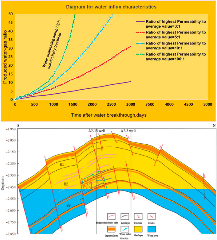
Figure 2. Water drive gas reservoirs and the recognition diagram of water influx modes (Huang et al., 2022).
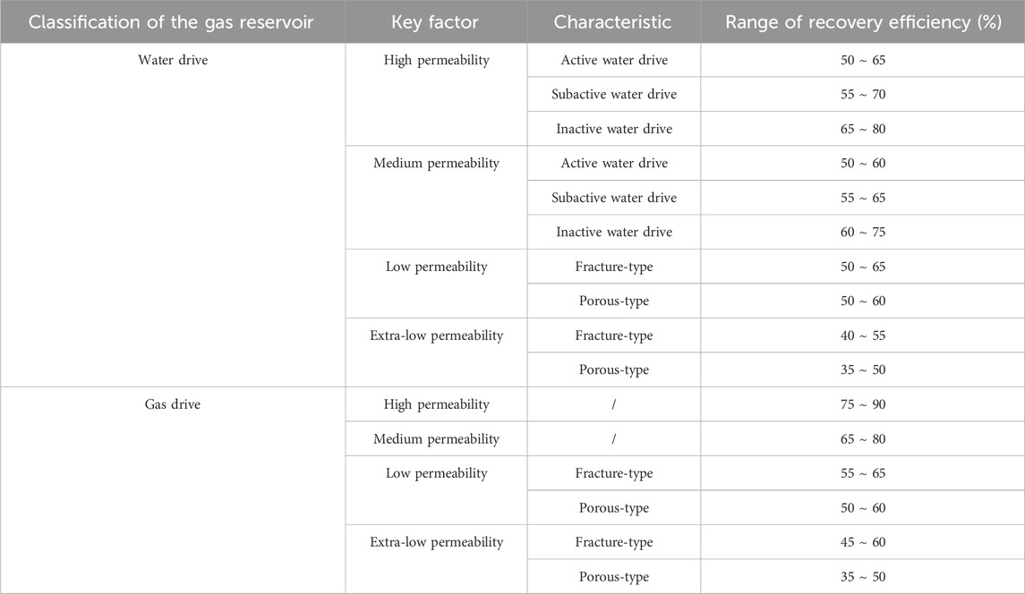
Table 1. Recovery efficiency of different gas reservoirs.
The national standard of the Classification of Oil and Gas Resources/Reserves (GB/T 19492-2004) (Administration, 2004) and the industry standard of the Code for Calculation of Oil and Gas Reserves (DZ/T0217-2005) (China, 2005) subdivide reserves into four categories: geological reserves, technically recoverable reserves, economically recoverable reserves, and remaining economically recoverable reserves (Wang et al., 2022). In Figure 3, the classification of development reserves clearly demonstrates the difference in various reserves. Technically, the recoverable reserve refers to the amount of natural gas that is expected to be eventually recovered from discovered gas reservoirs under current technical conditions and government regulations, also known as ultimate recoverable reserves, which is equal to the final cumulative production. Economically recoverable reserves refer to the amount of natural gas estimated and economically recoverable according to the current economic and technical conditions (price, cost, new investment, etc.). In the stage of submitting proved reserves, the technical recovery and economic recovery of the same type of gas reservoir are generally compared in China so as to demarcate the technical recoverable reserves and economic recoverable reserves of the gas reservoir. Scholars have made a more in-depth study on the calculation of recovery and recoverable reserves of water drive gas reservoirs. The calibration of recoverable reserves is the most important thing in exploration and development, and it is very meaningful for upstream oil and gas enterprises. Apart from mathematical algorithmic methods to calculate the recoverable reserves, through advanced deep learning technology, the accuracy and efficiency of reservoir recoverable reserve can also be improved (Deng et al., 2024).
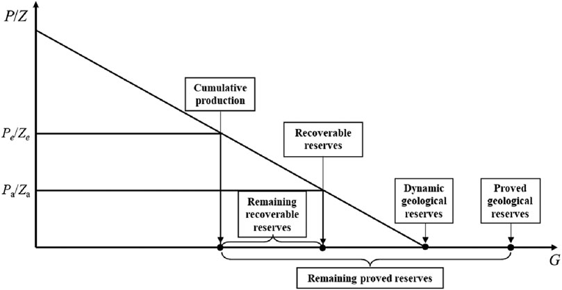
Figure 3. Classification of development reserves. P is the formation pressure, MPa; Z is the gas deviation factor, dimensionless; G is the gas reservoir geological reserves, m3; subscripts e and a are arbitrary conditions and abandonment conditions, respectively (Wei et al., 2021).
For water drive gas reservoirs, the calculation methods of recovery efficiency and recoverable reserves are various, which can be roughly divided into static and dynamic methods. These methods and equations are listed in Tables 2, 3.
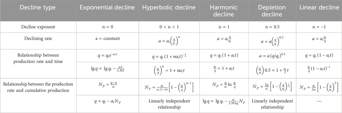
Table 2. Description of different production decline types.
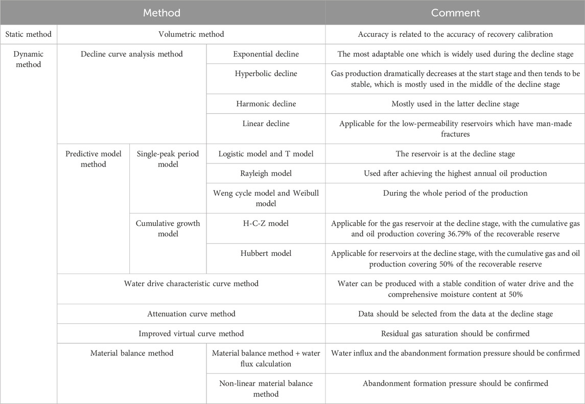
Table 3. Calculation methods of recoverable reserves of the gas reservoir.
2 The static method
2.1 The volumetric method
In the exploration and development stage of the gas reservoir, the static volume parameters of the reservoir (Xiao et al., 2013) are interpreted by using the obtained seismic, geological, drilling, coring, logging, oil testing, well testing, reservoir fluid sampling, and other data (Xiao et al., 2013) to calculate the original geological reserves of the gas reservoir. The calculation formula is given as follows in Eq. 1:
where G means geological reserves and A represents the gas reservoir area. h means formation thickness. ϕ means porosity of the formation. Sgi and Bgi represent the initial gas saturation of the reservoir and natural gas volume factor, respectively. pi means the original gas reservoir pressure, and psc means the standard pressure. T and Tsc represent the temperature of the gas reservoir and that under the standard condition, respectively. Zi is the natural gas initial deviation factor.
The recoverable reserves calculated by the volumetric method are the product of static geological reserves and recovery efficiency. The recoverable reserves of gas reservoirs can be preliminarily determined during the exploration and development stage by the method of calibrated recovery efficiency. The gas reservoir recovery efficiency can be calibrated by analogy and empirical formula methods, and the calculation accuracy depends on the matching degree between the gas reservoir type and empirical formula. The calculation principle of geological reserves by the volumetric method is to assume the gas reservoir is equivalent to an oil storage tank with a certain thickness and gas-bearing area. However, the formation condition of the actual gas reservoir is very complicated, and it is difficult to obtain accurate parameters of the reserves (such as effective thickness of the reservoir and gas-bearing area). Since there are many parameters used during calculation, the accuracy of the results depends on the accuracy of the parameters. The calibration of recovery efficiency includes empirical formula and analytical methods. The accuracy of the calculation results by the empirical formula method depends on the matching degree between the gas reservoir type and empirical formula. The analytical method is derived from the material balance method and is suitable for the gas reservoirs in the late stage of development.
The evaluation of reserves runs through the whole process of gas reservoir development. The prediction model can not only predict the production and recoverable reserves of the gas field but also predict the recoverable reserves increased due to development adjustment of the gas field, which is an important part of gas reservoir engineering. Decline curve analysis and water drive characteristic curve methods are common forecasting methods. However, the former method is only applicable to the decline stage during production, while the latter method is only applicable to the water drive gas reservoir, and the comprehensive water cut reaches more than 50%. This paper mainly discusses the forecast of the decline curve analysis method.
At present, many prediction models can be applied in forecasting the production and cumulative production of gas fields during the whole process, including the HCZ production model, Hubbert model, Weng cycle model, Class I generalized mathematical model, and Class II generalized mathematical model.
3 The dynamic methods
3.1 Successive subtraction of production method
Based on principles of mathematical statistics, the successive subtraction of production method, which is widely used by the reservoir engineers, can be applied to calculate recoverable and remaining reserves of reservoirs with the application of various distribution regularities (Chen et al., 2015; Chen, 2021). As early as 1908, Arnold and Anderson first proposed the concept of production decline. In 1921, Roswell H. Johnson introduced the concept to petroleum engineering and analyzed decline curves of several typical reservoirs. In 1945, J. J. Arps derived a series of different types of expressions of successive subtraction of production on the basis of empirical statistical models. Until today, the Arps successive subtraction curve method is still a prior method to predict the production and recoverable reserves in Western countries and also widely used in the middle-late stage of Chinese reservoirs. The most common methods of successive subtraction of production are presented in Table 1. There are several basic hypotheses when analyzing the successive subtraction curve:
(1) Comprehensive data on dynamic production can be provided, with a downward trend of production which boasts rationality and certainty.
(2) The trend of predicted production is in line with that of actual production.
(3) Economic limit has been clarified.
When assessing reserves, it is necessary for the estimator to consider factors that affect the characteristics of production decline, such as reservoir rock, fluid properties, unstable and stable flows, changes in the exploitation condition, and depletion mechanisms.
3.2 Water drive curve method
Although water drive gas does not equal water drive oil totally and the mechanisms are quite different, there is a semi-logarithmic linear relationship between cumulative gas production and cumulative water production in water drive gas reservoirs (LiZhang and Chen, 2010; Gou et al., 2013; Yao, 2016) in Eq. 2. Most publications state that the water drive curve method is only applicable for reservoirs at the mid-high water-cut stage. The water drive characteristic curve should be regressed, and a parallel line of production data should be selected to calculate the and the mechanisms are quite different, there is a semi-logarithmic recoverable reserve when applying practically in Eq. 3.
The corresponding cumulative gas production can be confirmed as the recoverable reserve when the water–gas ratio reaches the maximum:
3.3 Prediction model method
The mathematical model can be adopted to predict the recoverable reserve, aiming at the production change after reservoirs go into production in the prediction model method based on statistical laws (Yu et al., 2023).
Prediction model methods mainly fall into two categories, the unimodal periodic model and cumulative growth model, respectively, including the Weng cycle model in Eqs 5, 6, Logistic model in Eqs 7, 8, Rayleigh model in Eqs 9–11, Weibull model in Eq. 12, HCZ model in Eq. 13 and Hubbert model in Eq. 14.
(1) Weng cycle model:
(2) Logistic model:
(3) Rayleigh model:
(4) Weibull model:
(5) HCZ model:
(6) Hubbert model:
where Q is gas production per unit time and t is relative development time; the parameters a, b, and c are the constants of the prediction model, while Γ(b+1) means Γ(b+1) = b when b is a positive integer.
The actual production data are plugged into abovementioned models; then, the optimum model parameters can be confirmed to calculate the predicted recoverable production through regressing and fitting based on the linear trial and error.
3.4 Attenuation curve method
In 1995, Zhang proposed a new reciprocal attenuation equation (Pan, 2012) based on the attenuation curve studied by predecessors. This equation is convenient, accurate, and fast, and can quickly calculate the recoverable reserves of oil and gas fields in the decline period. The expression is as follows in Eqs 15, 16:
3.5 Improved virtual curve method
The relationship between pseudo-abandoned formation pressure and recoverable reserves can be derived from the reservoir volumetric calculation formula under original and abandoned conditions. The curve drawn by the formula is called the virtual curve. The p/Z and G relationship curves are drawn according to the dynamic production data on the water drive gas reservoir, and in the same figure as the virtual curve, the intersection point of the extension line of the decompression and reduction reserve curve and the virtual curve is found. The vertical coordinate of the intersection point is the pseudo-abandonment pressure value of the water drive gas reservoir, and the cumulative gas production corresponding to the horizontal coordinate of the intersection point is the recoverable reserve (Liu et al., 2007; WangChen and Zhang, 2017).
The natural gas surface volume under original conditions can be calculated through the following expression in Eq. 17.
Under abandoned conditions, the surface volume of remaining natural gas can be calculated through the following expression in Eq. 18.
Combining formula a and formula b, it is considered that the formation temperature remains unchanged in Eqs 19–21.
3.6 Material balance theoretical model of the gas reservoir
Experts at home and abroad have deduced various material balance equations, which are widely used to calculate the recoverable production.
In the whole process of gas reservoir production, the properties of fluid will change with the decrease in pressure. A general formula of the material balance equation can be established by using the theory of molar balance (Shi et al., 2022).
Based on the principle of molar balance, a general formula of the material balance equation for gas reservoirs with natural water drive and gas injection is established. After that, an analytical model can be proposed to calculate the maximum pressure threshold that can be induced with extra data based on the material balance equation (Cai and Dahi Taleghani, 2022). The assumptions are as follows: each component in the gas reservoir is homogeneous. The fluid properties at any time are determined by the formation pressure, and the pressure is in equilibrium at all places (Cai and Dahi Taleghani, 2021). The formation temperature is constant temperature. Ignoring capillary force and gravity in gas reservoir, the produced oil and gas uniformly come from different parts of the reservoir in Eq. 22.
Under the condition of known geological reserves, the size of recoverable reserves can be obtained by calculating the amount of water invasion combined with the abandonment pressure (Wei et al., 2020; Xue et al., 2022). Water influx and dynamic recoverable reserves are two critical parameters in the design of water drive gas reservoirs (Du et al., 2018). The expression of water influx can be derived based on water influx we have obatined. Evaluation of the intensity of water energy is applicable for further waterproof and water dealing (Hu et al., 2017; HuChen and Li, 2022).
The non-linear material balance method is based on the material balance equation of the water drive gas reservoir, and the empirical formula lnω = BlnR can be utilized to draw the theoretical chart of dimensionless apparent pressure and recovery degree of the water drive gas reservoir (HuLi and Songdai, 2013; Tan et al., 2021; Lv et al., 2022) in Eq. 23.
On the basis of the concept of plate fitting method and the dynamic production data, the actual and theoretical curves of the dimensionless pseudo-pressure and the recovery rate can be fitted successfully through adjusting the parameters (Xin et al., 2018; Ma et al., 2023).
This method can be utilized to make the theoretical chart of gas reservoir recovery degree and dimensionless pressure, where parameter B reflects the strength of water energy of water drive gas reservoirs. The general water drive condensate gas reservoir 1 < B<∞; the larger parameter B represents a weaker water energy. On the contrary, a smaller parameter B means stronger water energy. When B > 4.0, the water invasion is not quite severe. Only the pressure and cumulative production data are required to calculate dynamic reserve and water invasion directly in the non-linear material balance method. Meanwhile, the index of water drive intensity in gas reservoirs can also be confirmed.
Then, the recoverable reserves are calculated according to the recovery efficiency. This method is suitable for the dynamic reserve calculation of a single well or single pressure system. The results can be obtained by using the least square method to automatically fit the objective function of laminar flow pressure and cumulative production.
For water drive gas reservoirs with fractures, their geological reserves and recovery efficiency are difficult to evaluate. Unless there are good analog reservoirs, it is difficult to ensure that the evaluation results can be certain to use. For water drive gas reservoirs with fractures, some scholars consider water to seal gas on the basis of this method waiting to be improved (Tan et al., 2021). In order to clarify the characteristics of non-uniform water with slow speed in gas reservoirs with water and fractures, based on the dual action mechanism of water invasion and charging formation energy and gas in the blocked reservoir, and considering the development scale of fractures, the reservoir non-uniformity coefficient (A) is introduced to characterize the degree of reservoir physical non-uniformity. Then, a material balance method considering the phenomenon of water-sealed gas was established, and on this basis, the water invasion characteristic curve chart of gas reservoirs with water was drawn. The formula obtained is as follows in Eq. 24:
After fitting the production data, the fitted curve in Figure 4 can be obtained (Tan et al., 2021). On the basis of knowing the abandonment pressure, the recovery rate can be confirmed, and successively, the recoverable production can be calculated.
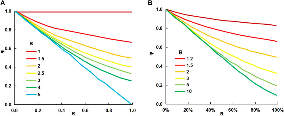
Figure 4. Chart of the non-linear material balance method (Tan et al., 2021).
4 Calculation example
There is a water drive gas reservoir controlled by a single well. In terms of the unstable well test in the field, core analysis, and the current production dynamics, the basic parameters of the single well and the gas reservoir are obtained herein.
The well radius Rw is 0.1 m, the reservoir thickness h is 44.4 m, the temperature of the reservoir T is 440.8 K, the relative density γg is 0.6972, the drainage radius Re is 967 m, the permeability of the reservoir K is 5.72 mD, the initial formation pressure pi is 42.14 MPa, the bottom hole pressure pwf is 13.16 MPa, the current production qsc is 4.06 × 10⁴ m3/d, water production qw is 16.26 m3/d, the deviation factor Z is 0.9, the initial volume factor Bgi is 0.004, the formation water volume factor Bw is 0.9909, the formation water compressibility factor Cw is 0.000641 MPa−1, the rock compressibility Cf is 0.000946 MPa−1, the current cumulative gas production Gp is 3.5461 × 10⁸ m3, the current cumulative water production Wp is 2.7558 × 10⁴ m3, and the connate water saturation Swi is 0.21. Meanwhile, the relative permeability curve of two phases of water and gas is demonstrated below in Figure 5.
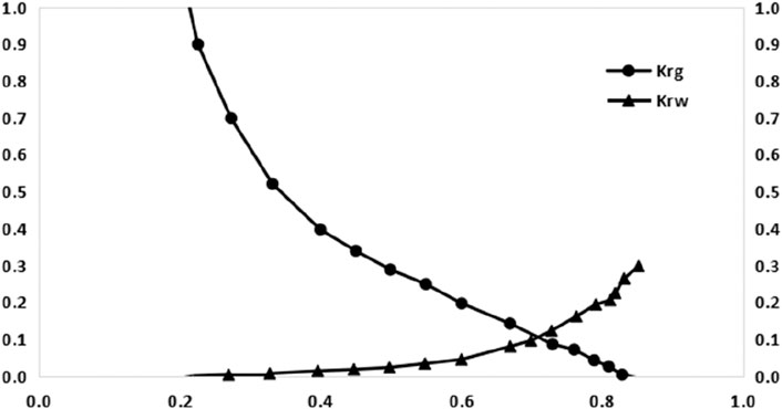
Figure 5. Gas–water two-phase relative permeability curve.
According to the actual production data and various parameters obtained, the relation curve between gas viscosity μg and pressure p can be drawn (Figure 6), and the relation formula can be fitted as well. In terms of the gas–water two-phase relative permeability curve, the corresponding relation of p with Krg and Sw can be calculated, and the charts are shown below. Although Krg and Sw change a lot when p < 5 MPa, yet Krg and Sw would have a linear change. In terms of field data, the current bottom flow pressure is 13.16 MPa and 42.14 MPa, so the current formation pressure range should be 13.16–42.14 MPa. Under the current formation pressure, Sw and Krg with p should meet the linear change, as shown in Figures 7, 8.
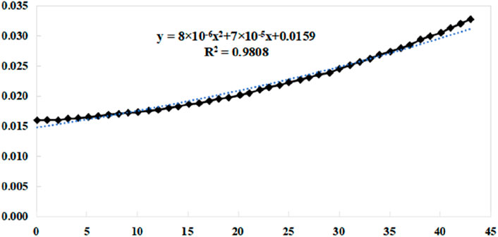
Figure 6. Relation curve between gas viscosity μg and pressure p.
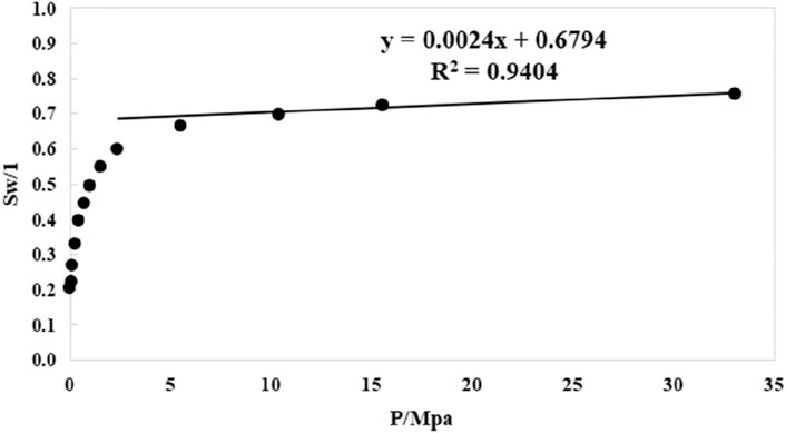
Figure 7. Relation curve between water saturation Sw and pressure p.
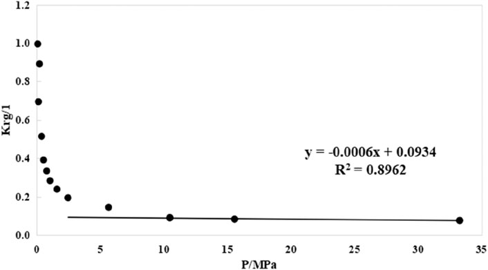
Figure 8. Relation curve between gas-phase relative permeability Krg and pressure p.
After calculation, we confirm that pR = 18.09 MPa and Bg = 7.65 × 10⁻³. Sw = 0.726 and Krg = 0.0912 can be obtained by using the fitting formula and utilizing the relative permeability curve.
In the formula we have listed, the calculation results of the current formation pressure, volume factor, and water saturation can be used to confirm the dynamic recoverable reserve of this water drive gas reservoir G = 4.64 × 10⁸ m3; the current water influx We is 9.85 × 10⁸ m3. The absolute error is just 0.83 × 10⁵ m3. It has proved a practical and highly accurate method to calculate the recoverable reserve of the water drive gas reservoir.
5 Conclusion
1. It is of vital importance for engineers and experts to confirm the recoverable reserves of deep water drive gas reservoirs, which is also complicated to establish. In this paper, multiple methods have been compared and analyzed for different situations, mainly including the static and dynamic methods. Selecting a suitable method is key to calculating the recoverable reserves of the deep water drive gas reservoirs accurately.
2. The static method includes the volumetric method, and the dynamic methods include the successive subtraction of production method, water drive curve method, prediction model method, attenuation curve method, improved virtual curve method, and material balance theoretical model of gas reservoirs.
3. When evaluating the recoverable reserve of deep water drive gas reservoirs at an early stage, the volumetric method can provide a relatively accurate result, which is utilized to confirm the development strategy and original plan. In the middle-late stage, the dynamic methods for calculating the recoverable reserve are essential for developing the gas reservoir effectively and appropriately. The material balance method is widely recognized as a high-accuracy method to calculate the recoverable reserves of deep water drive gas reservoirs.
Author contributions
QS: writing–original draft. CD: writing–review and editing. XW: writing–review and editing and investigation. QF: conceptualization and writing–original draft. QZ: resources and writing–review and editing. CY: investigation and writing–review and editing. LX: writing–review and editing. MY: writing–review and editing.
Funding
The author(s) declare that financial support was received for the research, authorship, and/or publication of this article. This work was supported by the basic and forward Science and Technology Project of PetroChina Company Limited “Research on reserve production balance analysis in domestic developed gas reservoirs and SEC reserve growth” (Contact No: 2022DJ7902).
Conflict of interest
The authors declare that the research was conducted in the absence of any commercial or financial relationships that could be construed as a potential conflict of interest.
The authors declare that this study received funding from the Basic and Forward Science and Technology Project of PetroChina Company Limited. The funder had the following involvement in the study: design, collection, analysis, and the writing of this article.
Publisher’s note
All claims expressed in this article are solely those of the authors and do not necessarily represent those of their affiliated organizations, or those of the publisher, the editors, and the reviewers. Any product that may be evaluated in this article, or claim that may be made by its manufacturer, is not guaranteed or endorsed by the publisher.
References
Administration, S. (2004). Classifications for reservoirs/reserves. Beijing: Standards Press of China.
Cai, Y., and Dahi Taleghani, A. (2021). Axial fracture initiation during diagnostic fracture injection tests and its impact on interpretations. Rock Mech. Rock Eng. 54, 5845–5865. doi:10.1007/s00603-021-02598-6
Cai, Y., and Dahi Taleghani, A. (2022). Using pressure changes in offset wells for interpreting fracture driven interactions (FDI). J. Petroleum Sci. Eng. 219, 111111. doi:10.1016/j.petrol.2022.111111
Chen, Y. (2021). Dynamic methods for estimating initial gas in-place and initial recoverable reserves in gas reservoirs—for the revised 《SY/T 6098—2010》. Nat. Gas Explor. Dev. 44, 1–12.
Chen, Y., Li, J., Li, Y., and Bi, H. (2015). Using decline constants from matching type curve to predict recoverable reserves of oil and gas reservoirs. China Offshore Oil Gas 27, 49–54.
China, M. O. L. A. R. O. T. P. S. R. O. (2005). Regulation of petroleum reserves estimation. Beijing: Standards Press of China.
Deng, Z., Zhou, D., Kang, Z., and Dong, H. (2024). Deep learning-based dynamic forecasting method and application for ultra-deep fractured reservoir production. Front. Energy Res. 12. doi:10.3389/fenrg.2024.1369606
Du, L., Wang, N., Chen, H., Zhang, M., and Li, F. (2018). Integrated method for calculating water influx and dynamic geological reserves in water-drive gas reservoirs. Nat. Gas. Geosci. 29, 1803–1808.
Gou, Y., Liu, H., Gao, S., Hu, Z., Xue, H., and Zhou, H. (2013). Research and application effect analysis on water-drive characteristic curve for water-drive gas reservoir. Oil Drill. Prod. Technol. 35, 63–65.
Huang, S., Liu, J., Sun, J., and Geng, M. (2022). Water invasion mode of carbonate gas reservoirs controlled by edge water: three invasion modes. Front. Energy Res. 10, 860527. doi:10.3389/fenrg.2022.860527
Hu, J., Li, X., and Songdai, S. (2013). A new method for dynamic reserves evaluation of water-drive gas reservoir. Nat. Gas. Geosci. 24, 628–632.
Hu, S., Li, J., Jiang, N., Yuan, Y., and Wan, X. (2017). Experimental study on dynamic reserves loss by water invasion in water-driven gas reservoirs. Special Oil Gas Reservoirs 24, 146–149.
Hu, Y., Chen, Y., and Li, T. (2022). The formation development and theoretical connotations of "overall water control of gas reservoir" technology in gas field development. Nat. Gas. Ind. 42, 10–20.
Liao, H., Xu, T., and Yu, H. (2024). Progress and prospects of EOR technology in deep, massive sandstone reservoirs with a strong bottom-water drive. Energy Geosci. 5, 100164. doi:10.1016/j.engeos.2023.100164
Li, L. (2021). Development of natural gas industry in China: review and prospect. Nat. Gas. Ind. 41, 1–11.
Li, S., Zhang, Y., and Chen, G. (2010). Forecast of beneficial exploration district of yanchang formation in zhenyuan-jingchuan area, ordos basin. J. Chongqing Univ. Sci. Technol. Sci. Ed. 12, 1–2+29.
Liu, S., Li, M., Wu, Y., and Yu, C. (2007). Easy determination of abandonment pressure and recoverable reserves for gas reservoirs with water drive. Offshore oil., 56–58.
Lv, Z., Tang, H., Liu, Q., Tang, Y., Wang, Q., Chang, B., et al. (2022). Dynamic evaluation method of water sealed gas for ultra-deep fractured tight gas reservoir in Kuqa Depression, Tarim Basin. Nat. Gas. Geosci. 33, 1874–1882.
Lv, Z., Zhang, J., Zhang, Y., Yan, B., Liu, Z., and Li, G. (2023). Reservoir connectivity of ultra-deep fractured tight sandstone gas reservoir and development enlightenment: taking Keshen 2 gas reservoir in Kuqa Depression of Tarim Basin as an example. FAULT-BLOCK OIL&GAS FIELD 30, 31–37+95.
Ma, B., Duan, Y., Zhang, Z., Zhu, L., Li, X., and Luo, L. (2023). Type-curve-based method for dynamic reserve estimate in deep geopressured water-drive gas reservoirs. J. Shaanxi Univ. Sci. 41, 103–109.
Pan, W. (2012). Correction for attenuation curve method in LOW permeability gas reservoir dynamic analysis application. J. Southwest Petroleum Univ. Sci. Technol. Ed. 34, 116–120.
Qiu, H., Wen, M., Wu, Y., Xing, X., Ma, N., Li, Z., et al. (2023). Experiments in huizhou buried-hill fractured condensate reservoirs in nanhai oilfield. Xinjiang Pet. Geol. 44, 84–92.
Shi, J.-T., Jia, Y.-R., Zhang, L.-L., Ji, C.-J., Li, G.-F., Xiong, X.-Y., et al. (2022). The generalized method for estimating reserves of shale gas and coalbed methane reservoirs based on material balance equation. Petroleum Sci. 19, 2867–2878. doi:10.1016/j.petsci.2022.07.009
Statistics, N. B. O. (2023). National bureau of statistics of China. Available at: https://data.stats.gov.cn/easyquery.htm?cn=C01.
Tan, X., Peng, G., Li, X., Chen, Y., Xu, X., Kui, M., et al. (2021). Material balance method and classification of non-uniform water invasion mode for gas reservoirs with water considering the effect of water sealed gas. Nat. Gas. Ind. 41, 97–103.
Wang, N., Chen, Q., and Zhang, W. (2017). CORRECTIONS OF THE ALGORITHMS FOR THE ABANDONED PRESSURE AND GEOLOGICAL RESERVES OF WATER DRIVEN GAS RESERVOIRS. Petroleum Geol. Oilfield Dev. Daqing 36, 98–101.
Wang, Y., Yang, T., Xu, X., Ju, X., and Hu, X. (2022). Characteristics of the proved new addition economic recoverable oil and gas reserves in China. China Pet. Explor. 27, 13–26.
Wei, Y., Jia, A., Xu, Y., and Fang, J. (2020). Progress on different reserve calculation methods in the whole life cycle of gas reservoir development. Nat. Gas. Geosci. 31, 1749–1756.
Wei, Y., Jia, A., Xu, Y., and Fang, J. (2021). Progress on the different methods of reserves calculation in the whole life cycle of gas reservoir development. J. Nat. Gas Geoscience 6, 55–63. doi:10.1016/j.jnggs.2021.04.001
Wu, Y., Yang, M., Li, M., Sun, Y., Zhang, Y., and Wang, H. (2020). Laws and models of water invasion in Kela 2 gas field. Xinjiang Pet. Geol. 41, 302–306.
Xiao, P., Liu, H., Yu, X., and Pang, J. (2013). Compution and analysis on affecting factors of recovery ratio of water - drive gas reservoir. J. Chongqing Univ. Sci. Technol. Nat. Sci. Ed. 15, 116–119.
Xie, K., Lu, X., Pan, H., Han, D., Hu, G., Zhang, J., et al. (2018). Analysis of dynamic imbibition effect of surfactant in microcracks of reservoir at high temperature and low permeability. SPE Prod. OPERATIONS 33, 596–606. doi:10.2118/189970-pa
Xie, K., Mei, J., Cao, W., Cao, B., Yao, L., Zhang, B., et al. (2022). Improving oil mechanism of polymer gel fracturing fluid based on filtration displacement. J. Petroleum Sci. Eng. 218, 111030. doi:10.1016/j.petrol.2022.111030
Xin, C., Wang, Y., Xu, Y., Shi, L., and Du, Y. (2018). Tight gas reservoir gynamic reserve calculation with modified flowing material balance. Special Oil Gas Reservoirs 25, 95–98.
Xue, T., Ji, Y., Cheng, L., Lv, C., Yang, Y., and Lan, Z. (2022). A new method for determining dynamic reserves and water energy in water drive gas reservoir. Petroleum Geol. Oilfield Dev. Daqing 41, 63–68.
Yao, J. (2016). Relationships among 4 types of water-drive characteristic curves and Arps decline curve. Xinjiang Pet. Geol. 37, 447–451.
Yu, G., Jing, X., Li, H., Fang, Y., and Luo, L. (2023). Quantitative risk evaluation on natural gas production based on peak prediction: an example from Sinian gas reservoirs, central Sichuan paleo-uplift. Nat. Gas Technol. Econ. 17, 74–81+86.
Zhang, J., Li, B., Zhou, W., Zhou, S., Zhu, J., Liu, C., et al. (2023). Development and EGR technologies of offshore gas fields in China. Nat. Gas. Ind. 43, 132–140.
Nomenclature
Keywords: underground energy, recoverable reserves, evaluation methods, water drive gas reservoir, material balance method, static and dynamic methods
Citation: Sun Q, Dai C, Wang X, Feng Q, Zhao Q, Yan C, Xu L and Yuan M (2024) Review about evaluation methods of recoverable reserves of deep water drive gas reservoirs in China. Front. Energy Res. 12:1403259. doi: 10.3389/fenrg.2024.1403259
Received: 19 March 2024; Accepted: 25 April 2024;
Published: 05 June 2024.
Edited by:
Feng Dong, China University of Geosciences, ChinaReviewed by:
Shilai Hu, Chongqing University of Science and Technology, ChinaWenyang Shi, Changzhou University, China
Copyright © 2024 Sun, Dai, Wang, Feng, Zhao, Yan, Xu and Yuan. This is an open-access article distributed under the terms of the Creative Commons Attribution License (CC BY). The use, distribution or reproduction in other forums is permitted, provided the original author(s) and the copyright owner(s) are credited and that the original publication in this journal is cited, in accordance with accepted academic practice. No use, distribution or reproduction is permitted which does not comply with these terms.
*Correspondence: Qiao Feng, ZmVuZ3FfaHpAcGV0cm9jaGluYS5jb20uY24=