A sensorless efficiency-optimizing vector control scheme for an induction motor drive

In this paper, an energy-saving scheme in rotor field-orientated vector control is developed for induction motor drives. The energy-saving scheme minimizes copper and core losses in induction motors, which are equally applicable to induction generators. In efficiency optimization, an optimal stator angular velocity is uniquely obtained, and consequently, a corresponding optimal slip at any given rotor speed is determined. The challenge of determining a reference for rotor flux linkage that guarantees the minimal copper and core loss regime is overcome by developing a load torque observer loop. The torque observer is developed alongside a rotor speed observer for a sensorless speed operation. The observed mechanical torque is further used to enhance the outer-loop rotor speed control that generates an electromagnetic torque command used in building the reference for the inner-loop stator current control. The results obtained justified the effective operation of the torque and rotor speed observer, which consequently verified the effective minimal electrical loss regime at the optimal stator angular velocity and optimal rotor flux linkage. The results are further compared to results obtained from the equivalent induction machine drive on a finite-set model predictive control (FS-MPC) scheme with the same values of the optimal stator angular velocity and optimal rotor flux linkage. The developed efficiency-optimized vector control scheme gave lower ripples in developed electromagnetic torque and dampened overshoot better during step change in load torque.

1 Introduction

Over the years, induction machines, particularly squirrel cage induction motors, have maintained dominance in various industrial manufacturing and domestic applications. The squirrel cage induction motors have been competitive machines of choice for industrial electric drives because they are very rugged, relatively cheaper, and have low maintenance requirements than the wound rotor type. However, induction machines in general should be operated in least loss regimes to avoid over-consumption of energy. Kirischen et al. (1987) stated that electric drives have the largest share of grid energy consumption in the world. Hence, improved efficiencies in energy utilization by induction motors yield tremendous savings, and consequently, they avail more energy to other consumers. As such, efficiency improvement in induction motors significantly contributes to reduction in production costs in the manufacturing sector. Other applications that benefit tremendously from efficiency optimization in induction motors include motor-driven compressors in heating, ventilation, and air conditioning (HVAC) systems and in electric vehicle applications (Ghozziandall et al., 2004; Sajedi et al., 2011).

Core (iron) and copper (resistive) losses are the main electrical losses, which must be tactically minimized for energy savings to occur significantly in an induction machine drive (Abrahamsen et al., 2001). Minimization of such electrical losses is more than often implemented via adjustable voltage and frequency/speed control methods. With the advent of power electronics inverters, adjustable speed drives have been more competitive in industrial automation than their fixed-speed counterparts, where reasonable efficiency can only be achieved at full load (Kirschen et al., 1984; Sul and Park, 1988; Kirschen et al., 1985; Vukosavic and Levi, 2003).

Several control techniques have been employed to improve the efficiency of induction motor drives (Abrahamsen et al., 1996). They are grouped into three major categories: simple state control (SSC) (Akin et al., 2004; Lascu and Trzynadlowski, 2004), loss model control (LMC) (Uddin and Nam, 2008; Olajube and Anubi, 2023; Uddin et al., 2019), and the search control (SC) algorithms (Rehman and Xu, 2011; Kastha and Bose, 1995; Choudhary et al., 2015). The LMC involves the use of a machine model to compute the losses by selecting an appropriate value of flux that minimizes these losses, and it is the fastest of the three methods. However, its major drawback is its sensitivity to parameter variations. The SSC, on the other hand, is the simplified version of the LMC that utilizes the state-space control technique, which may include observer design to estimate the value of the required flux for cost and loss minimization (Almeida et al., 2007). SC is devoid of parameter variations but suffers from torque ripples and slow convergence depending on the dimension of its dynamics (Vukosavic and Levi, 2003; Chakraborty and Hori, 2003; Blanusa, 2010). Prior knowledge of the machine parameters is also required by the SC method for proper variation of the flux to achieve an optimum operating condition. However, these methods can be hybridized or combined to forestall the shortcomings of the individual methods (Chakraborty and Hori, 2003; Blanusa, 2010; Qu et al., 2012; Stumper et al., 2013). A fuzzy logic control method was used in Kumar et al. (2014) for fast convergence of the search control technique and to prevent torque ripples. A neuro-fuzzy method was also used in Sousa et al. (1995) and Bose et al. (1997) to improve the fuzzy logic technique.

The convergence point for the least core loss in an induction machine will not necessarily correspond to the convergence point for the least copper loss, as the two losses attain their minimal values independently. Therefore, to achieve an operating regime where both losses can be considered adequately reduced, a compromise between the core and copper losses must be reached. A compromise will be reached where both losses intersect.

In this article, therefore, classical Jacobi is used as the loss minimization procedure to uniquely determine the point of intersection between the core and copper losses. Consequently, the loss minimization yielded an optimal rotor flux command and an optimal stator angular velocity that fixes operation to a constant slip operation. Hence, the loss minimization in this paper is implemented via the field-orientated vector control scheme. In general, vector control is a multivariable control scheme that can target more than one control objective, which has matured significantly over the years. It has capability for flux regulation used in efficiency improvement, which makes it very promising in industrial drives (Chakraborty and Hori, 2003; Ta-Cao and Hori, 2000; Chakraborty et al., 2003; Moreno-Eguilaz and Peracaula, 1999; Sousa et al., 1992). However, a major setback with vector control is sensitivity to system parameter mismatch (Balogun et al., 2021). Mismatched inductance in the cross-coupling terms of the inner loop current control was observed in Balogun et al. (2021) to majorly influence the stability of the system. The setback in such system parameter mismatch is mitigated in this article by increasing the gains of the proportional plus integral (PI) of the inner loop control, as shown in Balogun et al. (2021). Such a strategy is adopted herein to improve the resiliency of vector control to system parameter variation. Furthermore, observers will be introduced to eliminate the need for mechanical sensors for rotor speed and mechanical load torque. The observed mechanical torque variable will be fed forward to enhance the rotor speed control loop in obtaining the reference command for inner current loop control. Furthermore, a comparative analysis is done between the developed vector control and equivalent finite-set model predictive control (FS-MPC) on an equivalent induction machine.

The rest of the paper is arranged as follows: Sections 2 and 3 present the model of an induction machine and its steady-state analysis, respectively. Electrical loss minimization control laws are discussed in Section 4, while the design of the efficiency-optimizing dynamic control scheme is shown in Section 5. Section 6 focuses on the mechanical torque and rotor speed observer design. The results and comparative analyses are given in Section 7 along with the discussion, and the paper is concluded in Section 8.

2 Induction machine model

An inverter-fed squirrel cage induction motor is illustrated in Figure 1A. The dynamic model of the squirrel cage induction motor drive is given in Equation 1–11. In Equation 1, Equation 2, k_c = 1+(r_s/r_c), whereby the stator voltage equations account for the core loss with a core loss resistance r_c, as shown in Figure 1B. Therefore, i’_qs and i’_ds are the effective torque producing stator current, as defined in Balogun et al. (2021) and Gong et al. (2019). Therefore, they are referred to as the stator currents to avoid confusion in use of terms.

$v_{qs}=\frac{m_{qs}{v}_{dc}}{2}=r_s{i}_{qs}^{\prime }+k_{c}p{\lambda }_{qs}+k_c\omega {\lambda }_{ds}.(1)$

$v_{ds}=\frac{m_{ds}{v}_{dc}}{2}=r_s{i}_{ds}^{\prime }+k_{c}p{\lambda }_{ds}-k_c\omega {\lambda }_{qs}.(2)$

$v_{qr}=0=r_r{i}_{qr}+p{\lambda }_{qr}+\left(\omega -{\omega }_r\right){\lambda }_{dr}.(3)$

$v_{dr}=0=r_r{i}_{dr}+p{\lambda }_{dr}-\left(\omega -{\omega }_r\right){\lambda }_{qr}.(4)$

where

${\lambda }_{qs}=L_s{i}_{qs}^{\prime }+L_m{i}_{qr}.(5)$

${\lambda }_{ds}=L_s{i}_{ds}^{\prime }+L_m{i}_{dr}.(6)$

${\lambda }_{qr}=L_r{i}_{qr}+L_m{i}_{qs}^{\prime }.(7)$

${\lambda }_{dr}=L_r{i}_{dr}+L_m{i}_{ds}^{\prime }.(8)$

$p{\omega }_r=\frac{P}{2J}\left(T_e-T_m\right).(9)$

where

$T_e=\frac{3P{L}_m}{4L_r}\left({\lambda }_{dr}{i}_{qs}^{\prime }-{\lambda }_{qr}{i}_{ds}^{\prime }\right).(10)$

$C_{d}p{v}_{dc}=\frac{3}{2}\left(i_o-i_d\right)=\frac{3}{2}{i}_o-\frac{3}{4}\left(m_{qs}{i}_{qs}+m_{ds}{i}_{ds}\right).(11)$

Figure 1

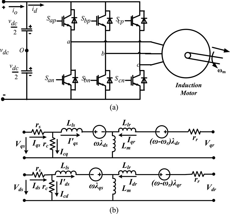
Figure 1. (A) An inverter-fed induction motor drive system. (B) q–d equivalent circuit model of the induction machine including core–loss resistance.

3 Steady-state analysis

In general, steady-state analysis is quite useful in establishing the operating and boundary regions in electric machines. Particularly, in squirrel cage induction motor drive, a regulation of the operational stator angular velocity (ω, in arbitrary reference frame) is of significant interest for achieving energy savings. At steady state, the derivative elements in the model of Section 2 are set to 0. Therefore, use of the steady states of Equations 3, 4 for appropriate substitution in rotor flux linkages in the T_e of the steady-state of Equation 9 yields Equation 12, which can be re-evaluated as Equation 13.

$T_e=T_m=\frac{3P}{4}\left(\frac{r_r{I}_r^2}{\left(\omega -{\omega }_r\right)}\right).(12)$

$I_r^2=\frac{4\left(\omega -{\omega }_r\right)}{3{\mathit{Pr}}_r}{T}_e=\frac{4\left(\omega -{\omega }_r\right)}{3{\mathit{Pr}}_r}{T}_m.(13)$

$P_L=\frac{3}{2}\left[\left({I_{qs}}^2+{I_{ds}}^2\right)r_s+\left({I_{qr}}^2+{I_{dr}}^2\right)r_r+\left({I_{cq}}^2+{I_{cd}}^2\right)r_c\right].(14)$

$P_L=\left(a_{PL}+\frac{b_{PL}\omega }{\left(\omega -{\omega }_r\right)}+\frac{c_{PL}}{{\left(\omega -{\omega }_r\right)}^2}\right)I_r^2.(15)$

Here, $a_{PL}=\frac{3}{2}\left[\frac{L_s}{L_m^2}\left(L_s^2\left(r_r-r_c\right)-r_r\right)-2L_s{L}_r\left(r_r+r_c\right)+r_r+r_s{L}_m+L_m^2{r}_c\right]$, $b_{PL}=\frac{3r_r{r}_s}{2r_c}$, and $c_{PL}=\frac{3}{2L_m^2}\left[r_s{r}_r^2\left(1+L_s^2\right)+r_c{L}_s^2\right]$.

The core and copper losses (P_L) of the machine are combined and given in Equation 14. The first two terms in Equation 14 give the copper loss, while the last term gives the core loss. The two loss regimes are embedded into Equation 14 so that two separate objective functions can be evaluated at once. If an induction machine is made to operate at constant slip when there is no magnetic saturation, as the rotor current increases, the stator angular velocity increases, and the copper loss increases while the core loss decreases. The two losses run contrary, as shown in Figure 2A. As such, a region of compromise must be reached where both loss functions intersect, which will be agreeable as optimal, as seen in Figure 2A. Consequently, at the point of intersection, the contribution of each of the loss function takes 50%, which implies that each of the copper loss and the core loss contributes equally to the total electrical losses at the optimal point. Therefore, Equation 14 is evaluated further as Equation 15, by appropriate substitution and simplification, to have reduced variable sets like Equation 12. By implication, substituting Equation 13 into Equation 15 gives the P_L as a quadratic function of ω, which gives rise to an optimization problem of minimizing the operational electrical losses at a corresponding stator angular velocity. As such, an optimization procedure that uniquely determines ω is given in the next section.

Figure 2

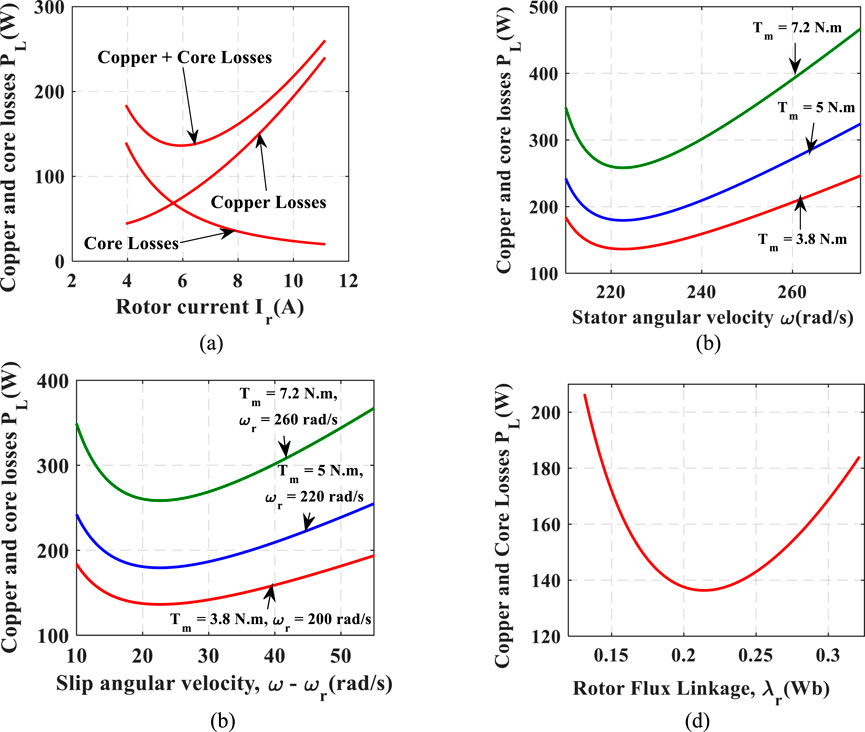
Figure 2. (A) Copper and core losses versus rotor current. (B) Copper and core losses versus stator angular velocity. (C) Copper and core losses versus slip angular velocity. (D) Copper and core losses versus rotor flux linkage.

In Figures 2B, C, profiles of the variation of P_L against stator angular velocity (ω) and against slip angular velocity (ωs) are given, respectively, at specified electromagnetic (T_e) or mechanical (T_m) torque and rotor speed (ω_r). The plots were obtained while the machine is constrained not to exceed the rated stator voltage and current (i.e., $V_s=\sqrt{V_{qs}^2+V_{ds}^2}\le V_{s\_rated}$ and $I_s=\sqrt{I_{qs}^2+I_{ds}^2}\le I_{s\_rated}$).

In Figure 2B, the rotor speed was specified at 200 rad/s for the random T_m at 3.8 N.m, 5 N.m, and 7.2 N.m. It can be seen in the figure that the least P_L at each of the given T_m coincides at the same ω of 224 rad/s. Therefore, there exists a constant slip angular velocity given as sω (where sω = ω - ω_r, obtained from slip s = ((ω - ω_r)/ω), which is 24 rad/s. As such, the constant slip operation for least P_L is further justified in Figure 2C, where the three given T_m in Figure 2B are subjected to random sub-synchronous ω_r. Consequently, the least P_L in each of the plot still coincides to 24 rad/s. In Figure 2D, the rotor flux linkage, regardless of the rotor speed, has a unique minimal value of 0.208 Wb that corresponds to less power loss. This value is observed to change only when the T_m (and consequently T_e) changes.

4 Electrical loss minimization control laws

In the previous section, the optimization problem was established as a control problem with an objective function of minimizing the copper and core losses of the induction machine with respect to the stator angular velocity and the rotor current magnitude. The goal is to investigate if a unique expression can be determined for an optimal stator angular velocity and consequently obtaining a unique expression for an optimal rotor flux linkage reference.

4.1 Determination of optimal stator frequency

The classical Jacobi is employed for the optimization procedure, which is formulated from the derivatives of P_L and T_e with respect to ω and I_r, as given in Equation 16. The objective (cost) function of Equation 16 is to minimize P_L, which also corresponds to maximizing the torque or power output of the machine. With the determinant of Equation 16 set to 0, Equation 17 is obtained as an optimal stator angular velocity that fixes the slip at an optimal value. The optimal stator angular velocity is critical for constant slip operation. As such, with machine parameters given in the appendix, Equation 17 gives ω_opt = 224 rad/s with rotor speed set at 200 rad/s, which corresponds to the value obtained as optimal in Figure 2B. Consequently, the terms in square root in the right-hand side of Equation 17 correspond to the slip angular velocity ωs, which is fixed at 24 rad/s according to the parameters of the test machine of this paper.

$\left|\begin{array}{cc}\frac{d{T}_e}{d{I}_r}& \frac{d{T}_e}{d\omega }\\ \frac{d{P}_L}{d{I}_r}& \frac{d{P}_L}{d\omega }\end{array}\right|=0.(16)$

${\omega }_{opt}={\omega }_r\pm \sqrt{\frac{A_c}{B_c}}.(17)$

Here, $A_c=r_c{r}_r^2\left(1+L_s^2\right)+r_c^2{r}_r^2{L}_s^2$ and $B_c=r_c{r}_s\left(1+L_s^2\right)L_r^2-2r_c{r}_s{L}_s{L}_r{L}_m^2+2r_s{r}_r{L}_m^2+r_c{r}_r{L}_m^2+r_c^2{L}_s^2{L}_r^2-2{r_c^{2}L}_s{L}_r{L}_m^2+r_c^2{L}_m^4$

4.2 Determination of optimal rotor flux linkage

With an optimal stator angular velocity obtained, a corresponding optimal rotor flux linkage reference can consequently be determined. Notice that at steady state of Equation 4 and with a rotor flux alignment of λ_qr = 0 and λ_dr = λ_r, I_dr = 0, consequently, I_qr = I_r. Therefore, the steady state of Equation 3, 18 is obtained, while Equation 19 is determined from Equation 13. As such, the corresponding optimal rotor flux linkage is given in Equation 20 as 0.208 Wb, with the mechanical torque specified as 3.8 N.m and with an optimal slip angular velocity obtained as 24 rad/s for this machine in the last sub-section. Therefore, based on Equation 20, the rotor flux agrees with Figure 2D and will only change along an optimal profile determined by a change in the mechanical torque.

${\lambda }_{dr}=-\frac{r_r{I}_{qr}}{{\omega }_{opt}-{\omega }_r}.(18)$

$I_{qr}=\sqrt{\frac{4T_m\left({\omega }_{opt}-{\omega }_r\right)}{3{\mathit{Pr}}_r}}.(19)$

${\mathit{\lambda }}_{\mathit{d}\mathit{r}\_\mathit{o}\mathit{p}\mathit{t}}=\pm \sqrt{\frac{\mathbf{4}{\mathit{T}}_{\mathit{m}}{\mathit{r}}_{\mathit{r}}}{\mathbf{3}\mathit{P}\left({\mathit{\omega }}_{\mathit{o}\mathit{p}\mathit{t}}-{\mathit{\omega }}_{\mathit{r}}\right)}}=\mathbf{0}.\mathbf{208}\hspace{0.33em}\mathit{W}\mathit{b}.(20)$

5 Efficiency-optimizing dynamic control scheme

The energy-saving dynamic control scheme is based on rotor flux-oriented vector control with inner-loop stator current control and outer-loop speed and rotor flux control. The rotor flux orientation of λ_qr = 0 and λ_dr = λ_r used in the previous section is adopted in the dynamic control. The flux alignment decouples inner-loop control of electromagnetic torque via independent control on the q-axis.

5.1 Inner-loop current control

The stator equations in Equations 1, 2 form the basis for the inner-loop control with the voltage impressed by the inverter as the stator control input vectors. As such, the stator flux linkages in Equations 1, 2 are expressed in terms of the rotor flux linkages and the stator current for the rotor field-oriented control. Consequently, Equation 21 is obtained as the dynamics of the inner-loop current regulation and expressed in complex form, as given in Equation 22.

$\left[\begin{array}{c}{L}_{\sigma }p{i}_{qs}+r{i}_{qs}\\ L_{\sigma }p{i}_{ds}+r{i}_{ds}\end{array}\right]=\left[\begin{array}{c}{\delta }_{qs}\\ {\delta }_{ds}\end{array}\right]=\left[\begin{array}{c}-\frac{{\omega }_r{L}_m{\lambda }_{dr}}{L_r}-\omega L_{\sigma }{i}_{ds}\\ \frac{r_r{L}_m}{{L_r}^2}{\lambda }_{dr}+\omega L_{\sigma }{i}_{qs}\end{array}\right]+\left[\begin{array}{cc}\frac{1}{k_c}& 0\\ 0& \frac{1}{k_c}\end{array}\right]\left[\begin{array}{c}{v}_{qs}\\ v_{ds}\end{array}\right].(21)$

$\left(L_{\sigma }p+r\right)i_{qds}=K_r\left(i_{qds}^{*}-i_{qds}\right)=K_r\left(e_{qds}\right)={\delta }_{qds}.(22)$

Here, $r=\left(r_s/k_c\right)+\left(r_r{L}_m^2/L_r^2\right)$ and $L_{\sigma }=L_s-L_m^2/L_r$.

$G_r\left(p\right)=\frac{i_{qs}}{K_{qr}{e}_{qs}}=\frac{i_{ds}}{K_{dr}{e}_{ds}}=\frac{1}{\left(p{L}_{\sigma }+r\right)}.(23)$

Expanding Equation 22 gives the open-loop current transfer function of Equation 23, where K_qr = K_dr = K_r and represents the proportional plus integral (PI) controllers in the inner-loop. The delay given in Equation 24 accounts for dead-time and transport/sampling delays introduced by the inverter feeding the machine and the analog-to-digital conversion process (Balogun et al., 2021; Dong and Ojo, 2006; Holmes et al., 2009; Kazmierkowski et al., 2002; Rabelo et al., 2009). Introducing Equations 24, 23 yields Equation 25. With the PI controller K_r expressed in terms of proportional and integral gains in Equation 26, the closed-loop transfer function of the plant’s inner-loop current control is given by Equation 27. For pole zero cancellation, the controller’s gains are selected such that K_pr/K_ir = L_σ/r (Lascu et al., 2007). Since inner-loop current controllers are the most significant in vector control stability (Ali et al., 2020), the stability of Equation 27 is sacrosanct.

$G_d\left(p\right)=\frac{1}{\left(p{T}_{rd}+1\right)}.(24)$

$G_r\left(p\right)G_d\left(p\right)=\frac{1}{\left(p{L}_{\sigma }+r\right)}\cdot \frac{1}{\left(p{T}_{rd}+1\right)}.(25)$

$K_r\left(p\right)=\frac{p{K}_{\mathit{pr}}+K_{ir}}{p}.(26)$

$G_{cr}\left(p\right)=\frac{K_{\mathit{pr}}}{\left(p^2{L}_{\sigma }{T}_{rd}+p{L}_{\sigma }+K_{\mathit{pr}}\right)}.(27)$

Comparing the denominator of Equation 27 with the second-order Butterworth polynomial of p²+2ω_nζp+ω_n² at optimal damping criteria, such that ζ = 1/√2, then ω_n/√2 = 1/T_rd and ω_n² = K_pr/(L_σ T_rd). Therefore, K_pr = L_σ/(2T_rd), and consequently, K_ir = r/(2T_rd). Hence, Equation 27 is further simplified as Equation 28. As such, the control inputs from the inverter are the stator voltage vectors given in Equation 29. δ_qs and δ_ds in Equation 29 stand for outputs from K_qr and K_dr in the q-axis and d-axis, respectively.

$G_{cr}\left(p\right)=\frac{i_{qs}}{{i_{qs}}^{*}}=\frac{i_{ds}}{{i_{ds}}^{*}}=\frac{1}{\left(p^{2}2{T_{rd}}^2+p2T_{rd}+1\right)}.(28)$

$\left[\begin{array}{c}{v}_{qs}\\ v_{ds}\end{array}\right]={\left[\begin{array}{cc}\frac{1}{k_c}& 0\\ 0& \frac{1}{k_c}\end{array}\right]}^{-1}\left[\left[\begin{array}{c}{\delta }_{qs}\\ {\delta }_{ds}\end{array}\right]-\left[\begin{array}{c}-\frac{{\omega }_r{L}_m{\lambda }_{dr}}{L_r}-\omega L_{\sigma }{i}_{ds}\\ \frac{r_r{L}_m}{{L_r}^2}{\lambda }_{dr}+\omega L_{\sigma }{i}_{qs}\end{array}\right]\right].(29)$

5.2 Outer-loop speed control

The rotor speed outer-loop control is developed from Equation 9 and obtained in Equation 30. With the rotor field orientation in the electromagnetic torque, as given in Equation 31, and accounting for friction and windage losses in Equation 9 via damping coefficient B_m, Equation 30 is expanded to Equation 32. Consequently, the q-axis stator current reference is generated in Equation 33. The current reference can also be represented by Equation 34 from Equation 28. As such, Equation 32 is modified to Equation 35. Equation 36 is obtained from Equation 3 and substituted in Equation 35 to yield Equation 37, which results in the open-loop transfer function of Equation 38. In the closed loop, Equation 39 evolves from Equation 38. K_ωr is the PI controller for the outer rotor speed loop, and δ_ωr stands for the output of K_ωr.

$\frac{2J}{P}p{\omega }_r=\left(T_e^{*}-T_m\right)=K_{\omega r}\left({\omega }_r^{*}-{\omega }_r\right)=K_{\omega }\left(e_{\omega }\right)={\delta }_{\omega }.(30)$

$T_e=\frac{3P{L}_m}{4L_r}{\lambda }_{dr}{i}_{qs}^{\prime *}.(31)$

$\frac{2J}{P}p{\omega }_r+\frac{2}{P}{B}_m{\omega }_r=\left(\frac{3P{L}_m}{4L_r}{\lambda }_{dr}{i}_{qs}^{\prime *}-T_m\right)=K_{\omega r}\left({\omega }_r^{*}-{\omega }_r\right)=K_{\omega r}\left(e_{\omega r}\right)={\delta }_{\omega r}.(32)$

$i_{qs}^{\prime *}=\frac{L_r}{k{\lambda }_r{L}_m}\left({\delta }_{{\omega }_r}+T_m\right).(33)$

$i_{qs}^{\prime *}=i_{qs}\left(p^{2}2{T_{rd}}^2+p2T_{rd}+1\right).(34)$

$K_{\omega r}\left({\omega }_r^{*}-{\omega }_r\right)=\frac{3P{L}_m}{4L_r}{\lambda }_{dr}{i}_{qs}\left(p^{2}2{T_{rd}}^2+p2T_{rd}+1\right)-T_m.(35)$

$i_{qs}=\frac{L_r}{L_m{r}_r}{\lambda }_r\left(\omega -{\omega }_r\right).(36)$

$K_{\omega r}\left({\omega }_r^{*}-{\omega }_r\right)=\frac{3P}{4r_r}{\lambda }_r^2\left(\omega -{\omega }_r\right)\left(p^{2}2{T_{rd}}^2+p2T_{rd}+1\right)-T_m.(37)$

${H_o}_{\omega r}=\frac{{\omega }_r}{K_{\omega r}\left({\omega }_r^{*}-{\omega }_r\right)}=\frac{{\omega }_r}{K_{\omega r}{e}_{\omega r}}=k_o\frac{1}{\left(p^{2}2{T_{rd}}^2+p2T_{rd}+1\right)}.(38)$

Here, $k_o=\frac{-3P}{4r_r}{\lambda }_r^2$.

${H_c}_{{\omega }_r}=k_o\frac{K_{\omega r}}{\left(p^{2}2{T_{rd}}^2+p2T_{rd}+1\right)\left(p{T}_{rc}+1\right)+k_o{K}_{\omega r}}.(39)$

In order make the controller’s zero cancel the undesired pole of the plant (Lascu et al., 2007), let the gains of the PI controller design in Equation 40 be selected as Equation 41 to yield Equation 42.

$K_{\omega r}=K_{p\omega r}+\frac{K_{i\omega r}}{p}.(40)$

$\frac{K_{p\omega r}}{K_{i\omega r}}=\frac{J}{B_m}.(41)$

$K_{\omega r}=\frac{K_{p\omega r}}{p{T}_{i\omega r}}\left(T_{i\omega r}p+1\right).(42)$

Here, $T_{i\omega r}=J/B_m$.

Hence, appropriate substitution of Equation 42 in Equation 39, while equating that $T_{i\omega r}=T_{rc}$ , $K_{p\omega r}=\frac{T_{rc}}{2k_o{T}_{rd}}$, and $k_o=\frac{-3P}{4r_r}{\lambda }_r^2$, yields the overall closed-loop transfer function of the speed control in Equation 43, given that all other disturbances are equated to 0. The linearized block model of the speed control loop is given in Figure 3.

${H_c}_{{\omega }_r}=\frac{1}{p^{3}4{T_{rd}}^3+p^{2}4{T_{rd}}^2+p2T_{rd}+1}.(43)$

Figure 3

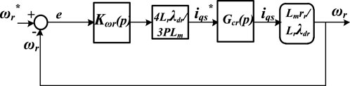
Figure 3. Linearized block model for rotor speed control loop.

5.3 Outer-loop optimized rotor flux linkage control

The rotor flux linkage is regulated at the outer-loop d-axis control of the inverter. Equation 44 evolves from Equation 4 and yields Equation 45 as the dynamics for the flux regulation. Therefore, Equation 28 yields Equation 46.

$L_{r}p{\lambda }_{dr}+r_r{\lambda }_{dr}=r_r{L}_m{i}_{ds}^{*}.(44)$

${\delta }_{\lambda r}=K_{\lambda r}\left({\lambda }_{dr}^{*}-{\lambda }_{dr}\right)=K_{\lambda r}\left(e_{\lambda r}\right)=\left(L_{r}p+r_r\right){\lambda }_{dr}=r_r{L}_m{i}_{ds}^{*}.(45)$

$i_{ds}^{*}=i_{ds}\left(p^{2}2{T_{rd}}^2+p2T_{rd}+1\right).(46)$

Here, K_λr represents the PI controller for the rotor flux outer-loop control and δ_λr stands for the output of K_λr. Substituting Equation 46 into Equation 45 yields Equation 47. However, from Equation 8, i’_ds can be represented as Equation 48, which can be substituted in Equation 47 to yield Equation 49.

${\delta }_{\lambda r}=L_m{r}_r{i}_{ds}^{\prime }\left(p^{2}2{T_{rd}}^2+p2T_{rd}+1\right).(47)$

$i_{ds}^{\prime }=\frac{1}{L_m}\left({\lambda }_{dr}-L_r{i}_{dr}\right).(48)$

$K_{\lambda r}\left({\lambda }_{dr}^{*}-{\lambda }_{dr}\right)=r_r\left({\lambda }_{dr}-L_r{i}_{dr}\right)\left(p^{2}2{T_{rd}}^2+p2T_{rd}+1\right).(49)$

Hence, the open-loop transfer function of the flux linkage controller given that all other disturbances are equated to zero gives Equation 50.

${H_o}_{\lambda r}=\frac{{\lambda }_r}{K_{\lambda r}\left({\lambda }_r^{*}-{\lambda }_r\right)}=\frac{{\lambda }_r}{K_{\lambda r}{e}_{{\lambda }_r}}=k_r\frac{1}{\left(p^{2}2{T_{rd}}^2+p2T_{rd}+1\right)},(50)$

where k_r = 1/r_r. Introducing a delay gain into Equation 50 results in Equation 51. The delay gain can represent the time constant of the filter needed for estimating the stator flux linkage.

${H_{oe}}_{\lambda r}=k_r\frac{1}{\left(p^{2}2{T_{rd}}^2+p2T_{rd}+1\right)\left(p{T}_{re}+1\right)}.(51)$

${H_c}_{\lambda r}=k_r\frac{K_{\lambda r}}{\left(p^{2}2{T_{rd}}^2+p2T_{rd}+1\right)\left(p{T}_{re}+1\right)+k_r{K}_{\lambda r}}.(52)$

The closed-loop transfer function is given in Equation 52. For pole-zero cancelation, let the PI controller design take the form K_pλr/K_iλr = L_r/r_r (Lascu et al., 2007). The gains of the PI controller are expressed in Equation 53, which translates to Equation 54.

$K_{\lambda r}=K_{p\lambda r}+\frac{K_{i\lambda r}}{p}.(53)$

$K_{\lambda r}=\frac{K_{p\lambda r}}{p{T}_i}\left(T_{i}p+1\right).(54)$

Here, $T_i=L_r/r_r$.

Hence, appropriate substitution of Equation 54 in Equation 52, while equating that $T_i=T_{re}$, $K_{p\lambda r}=T_{re}/\left(2k_r{T}_{rd}\right)$, and $k_r=1/r_r$, yields Equation 55.

${H_c}_{\lambda r}=\frac{1}{p^{3}4{T_{rd}}^3+p^{2}4{T_{rd}}^2+p2T_{rd}+1}.(55)$

Notice that Equation 55 is reduced to exactly the transfer function of Equation 43 for the speed control. The stability condition, therefore, that applies for the speed loop equally suffices for the rotor flux loop control based on gains selected for both loops. A linear model of the closed-loop flux regulation is shown in Figure 4. Figure 5 shows the pole’s loci for 3-time delays, T_rd = 2/f_s, 3/f_s, and 7/f_s (f_s = 5000 Hz, switching frequency of the converters), for the optimal damping criteria in Equations 43, 55. The system is seen to be stable at a natural frequency, ω_n, which decreases as T_rd increases. Consequently, with more increase of T_rd, the closer the poles are toward marginal stability. The practical implication as such is that with a significant increase in T_rd, the system is tossed into instability.

Figure 4

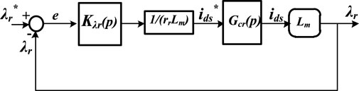
Figure 4. Linearized block diagram for the rotor flux linkage control loop.

Figure 5

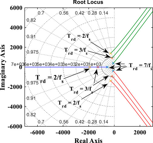
Figure 5. Loci of poles for Equations 43, 55 with T_rd = 3/f_s, 3/f_s, and 7/f_s.

6 Mechanical torque and rotor speed observer

The optimization procedure in Section 4 and the dynamic control scheme in Section 5 indicate that measuring or estimating the mechanical torque is quite vital for the efficiency optimization scheme of this article. State estimation (Awelewa et al., 2023; Omiloli et al., 2023) plays a significant role in this respect, as placing mechanical torque transducers on the drive will lead to an additional cost. Consequently, a Luenberger load torque observer is developed in this section for the energy saving scheme. The Luenberger observer block is included in the overall control scheme of the motor drive shown in Figure 6.

Figure 6

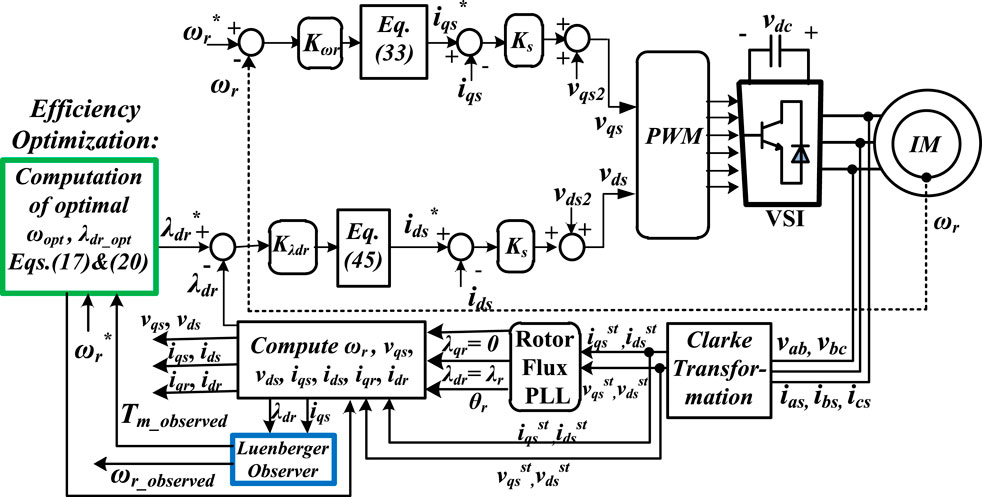
Figure 6. Block diagram of the overall control scheme on the motor drive.

6.1 State-space model

The mechanical dynamics of Equation 56 can be represented in the state-space format given in Equations 57, 58, where x = [x₁ x₂]^T =[ω_r T_m]^T, y = ω_r, u = i’_qs, and C = [1 0].

$\left[\begin{array}{c}{\dot{\omega }}_r\\ {\dot{T}}_m\end{array}\right]=\left[\begin{array}{cc}0& -\frac{P}{2J}\\ 0& 0\end{array}\right]\left[\begin{array}{c}{\omega }_r\\ T_m\end{array}\right]+\left[\begin{array}{cc}\frac{3P^2{L}_m{\lambda }_r}{8J{L}_r}& 0\\ 0& 0\end{array}\right]\left[\begin{array}{c}{i}_{qs}^{\prime }\\ 0\end{array}\right].(56)$

$\dot{x}=Ax+Bu.(57)$

$y=Cx.(58)$

Here, y = ω_r, u = i’_qs, $A=\left[\begin{array}{cc}0& -\frac{P}{2J}\\ 0& 0\end{array}\right]$, $B=\left[\begin{array}{cc}\frac{3P^2{L}_m{\lambda }_r}{8J{L}_r}& 0\\ 0& 0\end{array}\right]$, and $C=\left[\begin{array}{cc}1& 0\end{array}\right]$.

6.2 Observer model

The state-space model of sub-Section 6.1 is used to develop an observer for the mechanical load torque and consequently for the rotor speed as well. Consequently, a corresponding Luenberger observer model for Equation 56 is given in Equation 59, represented by the state-space of Equations 60, 61. Therefore, the observer herein is modified from Zorgani et al. (2016) for the rotor field-oriented control. The diagrammatic representation for the load torque and rotor speed Luenberger observer is shown in Figure 7.

$\left[\begin{array}{c}{\dot{\widehat{\omega }}}_r\\ {\dot{\widehat{T}}}_m\end{array}\right]=\left[\begin{array}{cc}0& -\frac{P}{2J}\\ 0& 0\end{array}\right]\left[\begin{array}{c}{\widehat{\omega }}_r\\ {\widehat{T}}_m\end{array}\right]+\left[\begin{array}{cc}\frac{3P^2{L}_m{\lambda }_r}{8J{L}_r}& 0\\ 0& 0\end{array}\right]\left[\begin{array}{c}{i}_{qs}^{\prime }\\ 0\end{array}\right]+\left[\begin{array}{c}{L}_1\\ L_2\end{array}\right]\left({\omega }_r-{\widehat{\omega }}_r\right).(59)$

$\dot{\widehat{x}}=A\widehat{x}+Bu+L\left(x-\widehat{x}\right).(60)$

$\widehat{y}=C\widehat{x}.(61)$

Figure 7

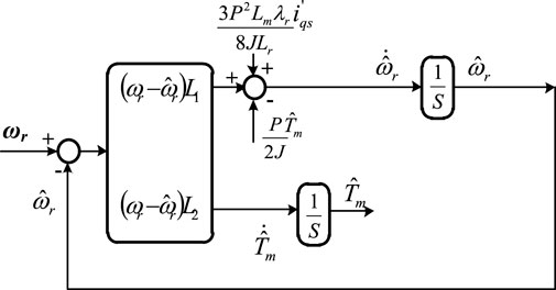
Figure 7. Block diagram of the Luenberger observer for load torque and rotor speed.

The error (e) between the actual state-space and state-observer models is given in Equation 62, where $\stackrel{\sim }{x}=e=x-\widehat{x}$. In the expanded form, Equation 62 translates to Equation 63.

$\dot{\stackrel{\sim }{x}}=\left(A-L\right)\stackrel{\sim }{x}.(62)$

$\left[\begin{array}{c}{\dot{\stackrel{\sim }{\omega }}}_r\\ {\dot{\stackrel{\sim }{T}}}_m\end{array}\right]=\left[\begin{array}{cc}-L_1& -\frac{P}{2J}\\ -L_2& 0\end{array}\right]\left[\begin{array}{c}{\stackrel{\sim }{\omega }}_r\\ {\stackrel{\sim }{T}}_m\end{array}\right].(63)$

$\left|\lambda I-{\left(A-L\right)}_{2\times 2}\right|=0.(64)$

The matrix (A–L) in Equation 62 and consequently Equation 63 gives the characteristic equation in Equation 64, which predicts the regions of stability (Awelewa et al., 2016) and instability (if any). Solving Equation 64 gives the loci of eigenvalues at a given operating condition. Specifically, Equation 64 is further evaluated as Equation 65 that bifurcates into two distinct roots given in Equation 66. As such, stability can only be guaranteed when the eigenvalues λ₁ and λ₂ given in Equation 66 are negative definite along the real axis of the eigenvalue locus. When L₁ is selected as positive values, L₂ must be selected as negative to maintain the negative definite eigenvalues in Equation 66. The stability limit of the observer, therefore, occurs at L₂ = 0, which locates λ₂ at the marginal stability of 0, while λ₁ is placed at a locus of -L₁. Making L₂ > 0 yields λ₂ to be positive definite and thereby throws the system into instability.

${\lambda }^2+L_1\lambda -\frac{L_{2}P}{2J}=0.(65)$

${\lambda }_1,{\lambda }_2=\frac{-L_1}{2}\pm \frac{\sqrt{L_1^2+\frac{4L_{2}P}{2J}}}{2}.(66)$

Figures 8A, B were obtained from Equation 64 and give the loci of the eigenvalues that indicate stable dynamics of the observer when L₁ is fixed at 50 and L₂ is varied from –0.1 to –40. Notice that at $L_1^2=-4L_{2}P/\left(2J\right)$, λ₁ and λ₂ become co-located on the real axis, and it implies that $L_2=-2J{L}_1^2/\left(4P\right)=-27.8125$ from the parameters given in Appendix A. Therefore, at L₂ = –27.8125 in Figures 8A, B, the loci of λ₁ and λ₂ can no longer extend further than –L₁/2 = –25 into the negative real axis but rather diverge into the imaginary axis as L₂ becomes more negative.

Figure 8

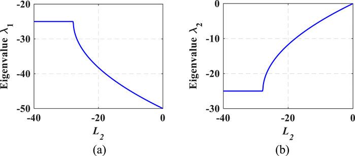
Figure 8. Eigenvalues from |λI-(A–L)_2x2| = 0: (A) real of eigenvalue loci of λ₁ against L₂. (B) Real of eigenvalue loci of λ₂ against L₂.

6.3 Primary rotor speed estimation for the observer model

Referring to (59), ${\widehat{\omega }}_r$ is the estimated rotor speed by the Luenberger observer, while ω_r could be the rotor speed measured by a speed encoder when only the mechanical torque is of interest for estimation. However, when both the mechanical torque and the rotor speed are desired to be observed, then ω_r in Equation 59 becomes an estimate from other means, as implied in Zorgani et al. (2016) when mechanical observers are not required. In consideration of the latter, a lower-order observer can be developed from Equation 3, as given in Equation 67, for ω_r, which can be substituted in Equation 59. The stator angular velocity, ω, may be determined by developing a flux phase-locked loop (flux PLL) that will give the slip angular velocity and corresponding slip angular displacement that will ensure that λ_qr = 0. Consequently, the reference rotor speed can be added to the slip angular velocity to extract out the precise ω and θ that achieves such an orientation. Alternatively, using Equation 3 to dynamically regulate the q-axis of the rotor flux linkage to 0 will give ω, such that ω_r in Equation 59 is taken as the rotor reference speed. The two methods have been explored during the project of this paper. However, the details of the two methods are not within the scope of this article.

${\omega }_{r\_est}=\omega +\frac{r_r{i}_{qr}}{{\lambda }_{dr}}.(67)$

7 Results and discussion

The dynamic sensorless efficiency optimization-based vector control with the torque observer developed in this paper for the induction motor drive was simulated in the MATLAB/Simulink environment. The simulation was carried out in two different operations. The results obtained for both operations are presented herein.

In the first operating condition, the reference rotor speed was set at 200 rad/s, while the load torque was set at 3.8 N.m. Under this condition, the rotor flux was set to pick its reference from the optimal value in Equation 20, which emanated from the optimization procedure. Then, at steady state between 4.5 s and 5.5 s, the rotor speed was ramped down from 200 rad/s to approximately 160 rad/s. After the duration of 2 s, the rotor speed was ramped back up to 200 rad/s between 7.5 s and 8.5 s. In Figures 9A–C, the rotor speed, load torque, and rotor flux linkage from the start-up to steady-state are shown. The Luenberger load torque observer gives the estimated rotor speed and estimated load torque in Figures 9A, B, respectively. In Figure 9A, the actual and observed ω_r are seen to follow the reference command closely despite the ramp from the reference. Similarly in Figure 9B, the estimated load torque can be seen to follow the actual value closely. In Figure 10A the ramped rotor speed is shown at steady state only.

Figure 9

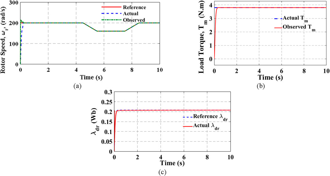
Figure 9. (A) Rotor speed: actual and estimated. (B) Load torque: actual and estimated. (C) Rotor flux linkage: reference and actual.

Figure 10

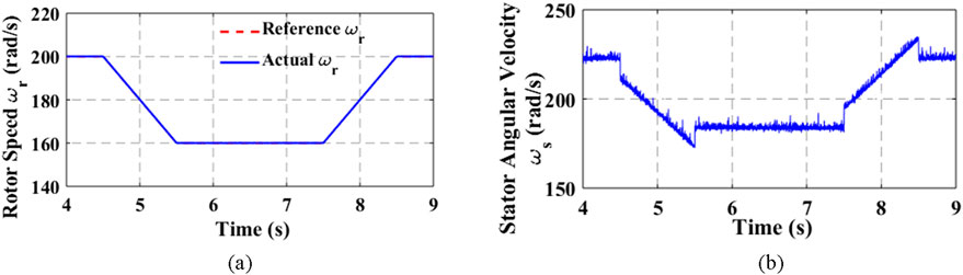
Figure 10. (A) Steady-state rotor speed: reference and actual. (B) Optimal stator angular velocity.

The corresponding stator angular velocity (ω_s) to Figure 10A that will guarantee optimal operation is shown in Figure 10B. The ω_s at the stator in Figure 10B is at a trajectory that gives a constant slip operation at the minimal copper and core loss regime. The q–d stator currents controlled in the inner-loop regulation are seen in Figures 11A, B respectively. Notice that in Figure 11A, the q-axis stator current maintained a steady value before and after the ramping down and ramping up. As such, a constant electromagnetic torque build-up is achieved for picking up the load torque that has been maintained constant. Therefore, it can be inferred in the optimization procedure developed that the load torque and not the rotor speed trajectory influences the choice of optimal rotor flux linkage. It can be deduced in the denominator of Equation 20 that if constant slip is maintained, as shown in Figures 11A, B, the load torque principally determines the choice of optimal rotor flux.

Figure 11

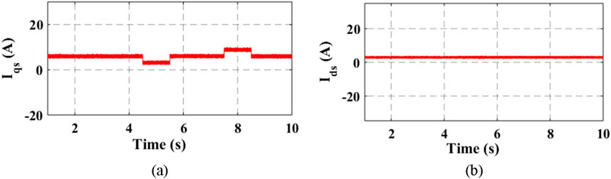
Figure 11. Stator current vectors (A) q-axis (B) d-axis.

In the second operation, the rotor speed and the load torque were maintained constant at 200 rad/s and 3.8 N.m, respectively, for the entire simulation. Then, the simulation was carried out with the rotor flux linkage set at the optimal value given in Equation 2 and later changed to values below and above the optimal. The reason for such is to investigate the influence of the rotor flux on the loss regime. Figures 12A–C give the loss regime for the three rotor flux values. In Figures 12A–C, therefore, the copper and core losses are seen to be less distorted in Figure 12A where the rotor flux linkage was set at optimal. As such, setting the rotor flux linkage to an optimal value conserves energy consumption by the induction motor.

Figure 12

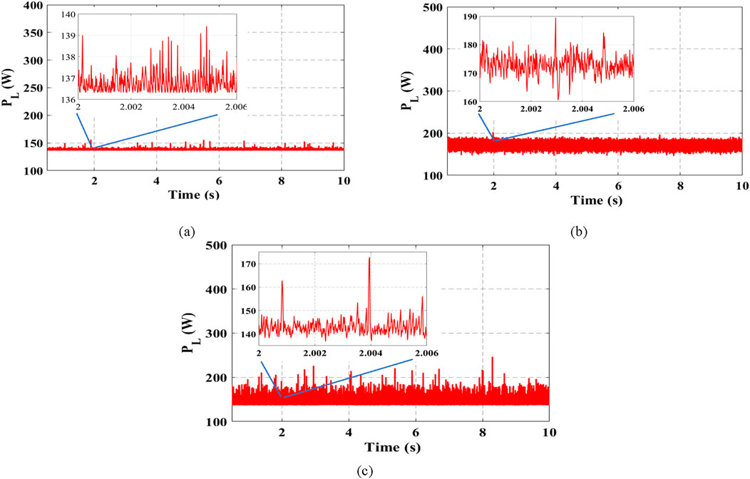
Figure 12. Copper and core losses when rotor flux linkage is (A) at optimal, λ_r = 0.208 Wb; (B) below optimal, at λ_r = 0.15 Wb; (C) above optimal, at λ_r = 0.25 Wb.

Furthermore, the efficacy of the developed efficiency-optimized vector control scheme was tested by comparing its results to those obtained from an equivalent induction machine drive on a model predictive control (MPC) scheme with the same set values of the optimal stator angular velocity and optimal rotor flux linkage. The MPC was developed in the stationary reference frame, but the details of developing the MPC are not within the scope of this article, but may be derived from previous studies (Agoro et al., 2018; Zhou et al., 2018; Mao et al., 2021; Rodas et al., 2021; Ouari et al., 2022; Wen et al., 2022; Yang et al., 2022; Liu et al., 2019; Zhang et al., 2019). Consequently, the stator currents and rotor currents in the developed energy-saving vector control scheme were transformed from the synchronous reference frame into the stationary reference frame for comparative analysis with those obtained from the MPC.

In obtaining the comparative results, the rotor speed was maintained constant at 200 rad/s, while the load torque was stepped from 5 N.m. to 3.8 N.m at 4 s. The stator currents, rotor currents, and electromagnetic torque obtained from the developed energy saving vector control scheme are shown in Figures 13, 14, 15A respectively. However, Figures 15B, 16, 17 show the electromagnetic torque, stator currents, and rotor currents. In comparing Figures 13–17, smooth transitions were noticed when the step change in the load torque was introduced from at 4 s. The vector control effectively dampened the overshoots, which were evident in the MPC. Moreover, the harmonic contents from the vector control scheme were not as significant as those from the MPC scheme. As such, the ripples in the electromagnetic torque from the vector control scheme shown in Figure 15A are much lower than those in Figure 15B from the MPC. The reason for such could be because the switching actions in the switching semiconductor devices (e.g., MOSFET and IGBT) of the inverter–motor drive on the vector control are symmetrical, but the switching actions by the MPC are asymmetrical, which could result in the more significant ripples in the machine’s electromagnetic torque from the MPC. However, it is seen from Figures 14, 17 that the rotor currents from MPC are lower than those from the vector control, which may be due to the cost function minimization inherent in the MPC that selects the optimal switching states that gives the minimal cost function. Consequently, more reduction in the electrical loss profile can still be experienced in the MPC, but the symmetrical switching in vector control gives the edge of healthier electromagnetic torque development.

Figure 13

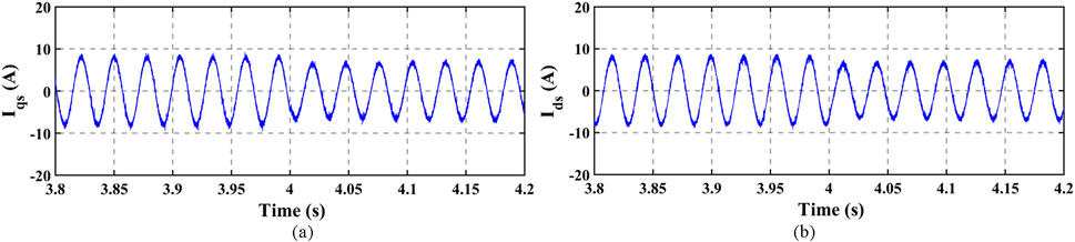
Figure 13. Stator stationary q–d reference frame currents in vector control: (A) I_qs and (B) I_ds.

Figure 14

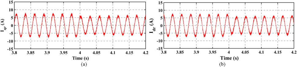
Figure 14. Rotor stationary q–d reference frame currents in vector control: (A) I_qr and (B) I_dr.

Figure 15

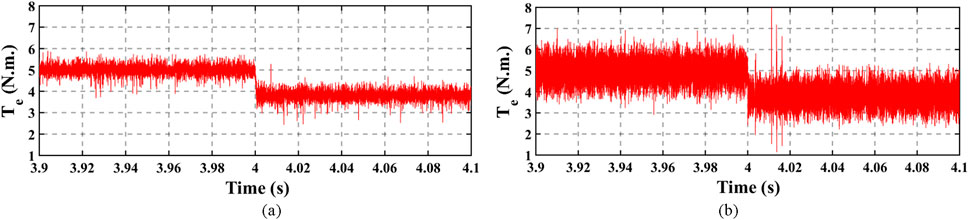
Figure 15. Electromagnetic torque: (A) from vector control and (B) from model predictive control.

Figure 16

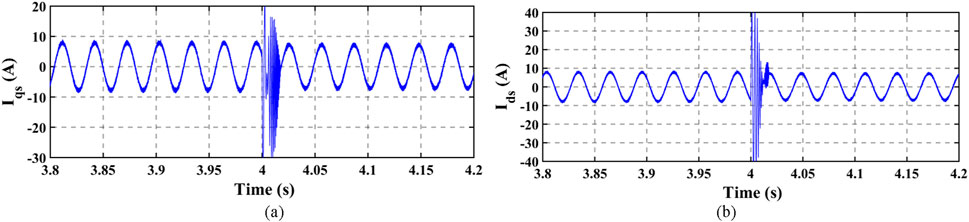
Figure 16. Stator stationary q–d reference frame currents in model predictive control: (A) I_qs and (B) I_ds.

Figure 17

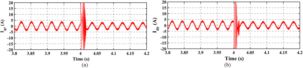
Figure 17. Rotor stationary q–d reference frame currents in model predictive control: (A) I_qr and (B) I_dr.

8 Conclusion

A vector control scheme for an induction motor drive has been presented in this paper. The scheme guarantees an optimal operating regime for the induction motor based on an appropriate choice of optimal reference for the rotor flux linkage, as any choice of the rotor flux linkage, which is above or below the optimal values, will lead to more copper and core losses and more harmonic distortions in the machine variables. Since the machine load torque aids the determination of this optimal reference, and the rotor speed does not play any active role in the choice of such optimal rotor flux linkage if the slip is maintained constant, a Luenberger observer is developed to estimate the load torque. In the comparative analysis with the MPC, though the energy-saving vector control yielded more rotor currents that may imply a slight increase in the loss regime, the vector control gave lower ripples and consequently healthier electromagnetic torque in the induction machine. Furthermore, the vector control scheme rode through the step change in load torque smoothly, which the MPC was unable to attain.

Data availability statement

The original contributions presented in the study are included in the article/Supplementary Material; further inquiries can be directed to the corresponding author.

Author contributions

AB: conceptualization, methodology, writing–original draft, and writing–review and editing. AO: investigation, methodology, software, and writing–review and editing. AA: funding acquisition, investigation, software, and writing–review and editing. FO: methodology, supervision, and writing–review and editing. TS: funding acquisition, investigation, software, and writing–review and editing. IS: funding acquisition, methodology, and writing–review and editing.

Funding

The author(s) declare that no financial support was received for the research, authorship, and/or publication of this article.

Acknowledgments

The authors acknowledge and appreciate technical support given to this project by the University of Lagos. The authors also deeply recognize the assistance given by Covenant University in all aspects of this research, especially the payment of the publication charges.

Conflict of interest

The authors declare that the research was conducted in the absence of any commercial or financial relationships that could be construed as a potential conflict of interest.

Publisher’s note

All claims expressed in this article are solely those of the authors and do not necessarily represent those of their affiliated organizations, or those of the publisher, the editors, and the reviewers. Any product that may be evaluated in this article, or claim that may be made by its manufacturer, is not guaranteed or endorsed by the publisher.

References

Abrahamsen, F., Blaabjerg, F., Pedersen, J. K., and Thoegersen, P. B. (2001). Efficiency-optimized control of medium-size induction motor drives. IEEE Trans. Ind. Appl. 37 (6), 1761–1767. doi:10.1109/28.968189

CrossRef Full Text | Google Scholar

Abrahamsen, F., Pedersen, J. K., and Blaabjerg, F. (1996). State-of-art of optimal efficiency control of low cost induction motor drives. Proc. PEMC 2, 163–170.

Google Scholar

Agoro, S., Balogun, A., Ojo, O., and Okafor, F. (2018). “Direct model-based predictive control of a three-phase grid connected VSI for photovoltaic power evacuation,” in proceedings of 9th IEEE International Symposium on Power Electronics for Distributed Generation Systems (PEDG), 1–6.

CrossRef Full Text | Google Scholar

Akin, B., Orguner, U., and Ersak, A. (2004). A comparative study on Kalman filtering techniques designed for state estimation of industrial AC drive systems. Proc. IEEE Int. Conf. Mechatronics, 2004. ICM '04. 12, 439–445. doi:10.1109/ICMECH.2004.1364479

CrossRef Full Text | Google Scholar

Ali, M. T., Zhou, D., Song, Y., Ghandhari, M., Harnefors, L., and Blaabjerg, F. (2020). Analysis and mitigation of SSCI in DFIG systems with experimental validation. IEEE Trans. Energy Convers. 35 (2), 714–723. doi:10.1109/tec.2019.2953976

CrossRef Full Text | Google Scholar

Almeida, D. D. S., Filho, W. C. P. D. A., and Sausa, G. C. D. (2007). Adaptive fuzzy controller for efficiency optimization of induction motors. IEEE transaction Industial Mot. 54 (4), 2157–2164.

Google Scholar

Awelewa, A., Omiloli, K., Samuel, I., Ojajube, A., and Popoola, O. (2023). Robust hybrid estimator for the state of charge of a lithium-ion battery. Front. Energy Res. 10, 1–11. doi:10.3389/fenrg.2022.1069364

CrossRef Full Text | Google Scholar

Awelewa, A. A., Awosope, C. O. A., Abdulkareem, A., and Samuel, I. (2016). Nonlinear control laws for electric power system stabilization. J. Eng. Appl. Sci. 11 (7), 1525–1531.

Google Scholar

Balogun, A., Ojo, O., and Okafor, F. (2021). Efficiency optimization control of doubly-fed induction generator transitioning into shorted-stator mode for extended low wind speed application. IEEE Trans. Industrial Electron. 68 (12), 12218–12228. doi:10.1109/tie.2020.3037990

CrossRef Full Text | Google Scholar

Blanusa, B. (2010). New trends in efficiency optimization ofinduction motor drives. bosnia and herzegovina: university of banja luka.

Google Scholar

Bose, B. K., Patel, N. R., and Rajashekara, K. (1997). A neuro-fuzzy-based online efficiency optimization control of a stator flux-oriented direct vectorcontrolled induction motor drive. IEEE Trans. Ind. Electron. 44 (2), 270–273. doi:10.1109/41.564168

CrossRef Full Text | Google Scholar

Chakraborty, C., and Hori, Y. (2003). Fast efficiency optimization techniques forthe indirect vector-controlled induction motor drives. IEEE Trans. Ind.Appl. 39 (4), 1070–1076. doi:10.1109/tia.2003.814550

CrossRef Full Text | Google Scholar

Chakraborty, C., Ta, M. C., and Hori, Y. (2003). Speed sensorless, efficiency optimized control of induction motor drives suitable for EV applications. Proc. IEEE IECON 1, 913–918. doi:10.1109/iecon.2003.1280105

CrossRef Full Text | Google Scholar

Choudhary, P. K., Dubeyand, S. P., and Gupta, V. K. (2015). Efficiency optimization of induction motor drive at steady-state condition. 2015 Int. Conf. Control, Instrum. Commun. Comput. Technol. (ICCICCT) 54, 470–475. doi:10.1109/ICCICCT.2015.7475325

CrossRef Full Text | Google Scholar

Dong, G., and Ojo, O. (2006). Efficiency optimizing control of induction motor using natural variables. IEEE Trans. Industrial Electron. 53 (6), 1791–1798. doi:10.1109/tie.2006.885117

CrossRef Full Text | Google Scholar

Ghozziandall, S., Jelassi, K., and Roboam, X. (2004). Energy optimization of induction motor drives. IEEE Int. Conf. Industrial Technol. (ICIT) 2, 602–610. doi:10.1109/icit.2004.1490143

CrossRef Full Text | Google Scholar

Gong, C., Hu, Y., Ni, K., Liu J, J., and Gao, J. (2019). SM load torque observer-based FCS-MPDSC with single prediction horizon for high dynamics of surface-mounted PMSM. IEEE Trans. Power Electron. 35 (1), 20–24. doi:10.1109/tpel.2019.2929714

CrossRef Full Text | Google Scholar

Holmes, D. G., Lipo, T. A., Kong, W. Y., and McGrath, B. P. (2009). Optimized design of stationary frame three phase AC current regulators. IEEE Trans. Power Electron. 24 (11), 2417–2426. doi:10.1109/tpel.2009.2029548

CrossRef Full Text | Google Scholar

Kastha, D., and Bose, B. K. (1995). On-line search based pulsating torque compensation of a fault mode single-phase variable frequency induction motor drive. IEEE Trans. Industry Appl. 31 (4), 802–811. doi:10.1109/28.395290

CrossRef Full Text | Google Scholar

Kazmierkowski, M. P., Krishnan, R., and Blaabjerg, F. (2002). Control in power electronics: selected problems. London: Acad. Press, 190–207.

Google Scholar

Kirischen, D. S., Novoty, D. W., and Lipo, T. A.March (1987). Optimal efficiency control of an induction motor drive. IEEE Trans. Energy Convers. EC-2 (1), 70–76. doi:10.1109/tec.1987.4765806

CrossRef Full Text | Google Scholar

Kirschen, D. S., Novotny, D. W., and Lipo, T. A. (1985). On line efficiency optimization of a variable frequency induction-motor drive. IEEE Trans. Ind. Appl. IA-21 (3), 610–616. doi:10.1109/tia.1985.349717

CrossRef Full Text | Google Scholar

Kirschen, D. S., Novotny, D. W., and Suwanwisoot, W. (1984). Minimizing induction motor losses by excitation control in variable frequency drives. IEEE Trans. Ind. Appl. IA-20 (5), 1244–1250. doi:10.1109/tia.1984.4504590

CrossRef Full Text | Google Scholar

Kumar, N., Chelliah, T. R., and Srivastava, S. S. (2014). Adaptive control schemes for improving dynamic performance of efficiency-optimized induction motor drives. ISA Trans. 57, 301–310.

PubMed Abstract | CrossRef Full Text | Google Scholar

Lascu, C., Asiminoaei, L., Boldea, I., and Blaabjerg, F. (2007). High performance current controller for selective harmonic compensation in active power filters. IEEE Trans. Power Electron. 22 (5), 1826–1835. doi:10.1109/tpel.2007.904060

CrossRef Full Text | Google Scholar

Lascu, C., and Trzynadlowski, A. M. (2004). Combining the principles of sliding mode, direct torque control, and space-vector modulation in a high-performance sensorless AC drive. IEEE Trans. Industry Appl. 40 (1), 170–177. doi:10.1109/TIA.2003.821667

CrossRef Full Text | Google Scholar

Liu, M., Chan, K. W., Hu, J., Xu, W., and Rodriguez, J. (2019). Model predictive direct speed control with torque oscillation reduction for PMSM drives. IEEE Trans. Industrial Inf. 15 (9), 4944–4956. doi:10.1109/tii.2019.2898004

CrossRef Full Text | Google Scholar

Mao, J., Li, H., Yang, L., Zhang, H., Liu, L., Wang, X., et al. (2021). Non-cascaded model-free predictive speed control of SMPMSM drive system. IEEE Trans. Energy Convers. 37 (1), 153–162. doi:10.1109/tec.2021.3090427

CrossRef Full Text | Google Scholar

Moreno-Eguilaz, J. M., and Peracaula, J. (1999). Efficiency optimization for induction motor drives: past, present and future. Proc. Electrimacs, I.187–I.191.

Google Scholar

Olajube, A., and Anubi, O. M. (2023). “Model-based loss minimization control of a squirrel cage induction motor drive with shorted rotor under indirect field orientation,” in 2023 IEEE Conference on Control Technology and Applications (CCTA), Bridgetown, Barbados (IEEE), 759–765.

CrossRef Full Text | Google Scholar

Omiloli, K., Awelewa, A., Samuel, I., Obiazi, O., and Katende, J. (2023). State of charge estimation based on a modified extended Kalman filter. Int. J. Electr. Comput. Eng. 13 (5), 5054–5065. doi:10.11591/ijece.v13i5.pp5054-5065

CrossRef Full Text | Google Scholar

Ouari, K., Belkhier, Y., Djouadi, H., Kasri, A., Bajaj, M., Alsharef, M., et al. (2022). Improved nonlinear generalized model predictive control for robustness and power enhancement of a DFIG-based wind energy converter. Front. Energy Res. 10, 996206. doi:10.3389/fenrg.2022.996206

CrossRef Full Text | Google Scholar

Qu, Z., Ratna, M., Hinkkanen, M., and Luomi, 1. (2012). Loss-minimizing flux level control of induction motor drives. IEEE Trans. Ind. Appl. 48, 952–961. doi:10.1109/tia.2012.2190818

CrossRef Full Text | Google Scholar

Rabelo, B. C., Hofmann, W., da Silva, J. L., Gaiba de Oliveira, R., and Rocha Silva, S. (2009). Reactive power control design in doubly fed induction generators for wind turbines. IEEE Trans. Industrial Electron. 56 (10), 4154–4162. doi:10.1109/tie.2009.2028355

CrossRef Full Text | Google Scholar

Rehman, H., and Xu, L. (2011). Alternative energy vehicles drive system: control, flux and torque estimation, and efficiency optimization. IEEE Trans. Veh. Technol. 60 (8), 3625–3634. doi:10.1109/TVT.2011.2163537

CrossRef Full Text | Google Scholar

Rodas, J., Gonzalez-Prieto, I., Kali, Y., Saad, M., and Doval-Gandoy, J. (2021). Recent advances in model predictive and sliding mode current control techniques of multiphase induction machines. Front. Energy Res. 9, 729034. doi:10.3389/fenrg.2021.729034

CrossRef Full Text | Google Scholar

Sajedi, S., Khalifeh, F., Khalifeh, Z., and karimi, T. (2011). Application of Particle swarm Optimization and Genetic Algorithm methods for vector control of induction motor. Aust. J. Basic Appl. Sci. 5 (12), 1697–1706.

Google Scholar

Sousa, G. C. D., Bose, B. K., and Cleland, J. G. (1995). Fuzzy logic based on-line efficiency optimization control of an indirect vector-controlled induction motor drive. IEEE Trans. Ind. Electron. 42 (2), 192–198. doi:10.1109/41.370386

CrossRef Full Text | Google Scholar

Sousa, G. C. D., Bose, B. K., Cleland, J. G., Spiegel, R. J., and Chappell, P. J. (1992). Loss modeling of converter induction machine system for variable speed drive. Proc. IEEE IECON 115, 114–120. doi:10.1109/iecon.1992.254595

CrossRef Full Text | Google Scholar

Stumper, J. F., Dotlinger, A., and Kennel, R. (2013). Loss minimization of induction machines in dynamic operation. IEEE Trans. energy Convers. 28 (3), 726–735. doi:10.1109/tec.2013.2262048

CrossRef Full Text | Google Scholar

Sul, S. K., and Park, M. H. (1988). A novel technique for optimal efficiency control of a current source inverter fed induction motor. IEEE Trans. Power Electron. 3 (2), 192–199. doi:10.1109/63.4349

CrossRef Full Text | Google Scholar

Ta-Cao, M., and Hori, Y. (2000). “Convergence improvement of efficiency optimization control of induction motor drives,” in Proc. IEEE IASAnnu.Meeting, Rome, Italy.

Google Scholar

Uddin, M. N., and Nam, S. W. (2008). Development of a nonlinear and model-based online loss minimization control of an IM drive. IEEE Trans. Energy Convers. 23 (4), 1015–1024. doi:10.1109/TEC.2008.2001442

CrossRef Full Text | Google Scholar

Uddin, M. N., Rahman, M. M., Patel, B., and Venkatesh, B. (2019). Performance of a loss model based nonlinear controller for IPMSM drive incorporating parameter uncertainties. IEEE Trans. Power Electron. 34 (6), 5684–5696. doi:10.1109/TPEL.2018.2871033

CrossRef Full Text | Google Scholar

Vukosavic, S. N., and Levi, E. (2003). Robust DSP-based efficiency optimization of a variable speed induction motor drive. IEEE Trans. Ind. Electron. 50 (3), 560–570. doi:10.1109/tie.2003.812468

CrossRef Full Text | Google Scholar

Wen, X., Wu, T., Jiang, H., Peng, J., and Wang, H. (2022). MPC-based control strategy of PV grid connected inverter for damping power oscillations. Front. Energy Res. 10, 968910. doi:10.3389/fenrg.2022.968910

CrossRef Full Text | Google Scholar

Yang, L., Li, H., Huang, J., Zhang, Z., and Zhao, H. (2022). Model predictive direct speed control with novel cost function for SMPMSM drives. IEEE Trans. Power Electron. 37 (8), 9586–9595. doi:10.1109/tpel.2022.3155465

CrossRef Full Text | Google Scholar

Zhang, X., Cheng, Y., Zhao, Z., and He, Y. (2019). Robust model predictive direct speed control for SPMSM drives based on full parameter disturbances and load observer. IEEE Trans. Power Electron. 35 (8), 8361–8373. doi:10.1109/tpel.2019.2962857

CrossRef Full Text | Google Scholar

Zhou, Y., Li, H., and Zhang, H. (2018). Model-free deadbeat predictive current control of a surface-mounted permanent magnet synchronous motor drive system. J. Power Electron. 18 (1), 103–115.

Google Scholar

Zorgani, Y. A., Koubaa, Y., and Boussak, M. (2016). MRAS state estimator for speed sensorless ISFOC induction motor drives with Luenberger load torque estimation. ISA Trans. 61, 308–317. doi:10.1016/j.isatra.2015.12.015

PubMed Abstract | CrossRef Full Text | Google Scholar

Appendix

Machine parameters

A 3 hp, 1,710 rpm, 220–V line-line (rms), 60 Hz, 4-pole squirrel cage induction machine; stator resistance (r_s) 0.435 Ω; rotor referred resistance (r_r) 0.816 Ω; stator leakage inductance (L_ls) 0.002 H; rotor referred leakage inductance (L_lr) 0.002 H; magnetizing inductance (L_m) 0.0693 H; core loss resistance (r_c) 850 Ω; inertia (J) 0.089 kg.m²; rated torque 11.9 N.m.

Nomenclature

v_qs, v_ds q and d stator voltages

i_qs, i_ds q and d stator currents

${\mathit{i}}_{\mathit{q}\mathit{s}}^{\prime }$,${\mathit{i}}_{\mathit{d}\mathit{s}}^{\prime }$ Torque producing q and d stator currents

λ_qs, λ_ds q and d stator flux linkages

v_qr, v_dr q and d stator referred rotor voltages

i_qr, i_dr q and d stator referred rotor currents

λ_qr, λ_dr q and d stator referred rotor flux linkages

i_cq, i_cd q and d core loss currents

ω, ω_e Angular velocity in arbitrary and synchronous frames

ω_r, ω_s Rotor speed and stator angular velocity

L_s, L_r Stator and stator referred rotor self-inductances

r_s, r_r Stator and stator referred rotor resistance

r_c Core loss resistance

L_m Magnetizing inductance (3/2 in value)

VSI Voltage source inverter

T_e, T_m Electromagnetic torque and mechanical torque

P_L Core and copper losses

m_qr, m_dr VSI’s q and d modulation index for CB-PWM

v_dc direct current (DC) link voltage

C_d DC link capacitor

i_o Rectifier’s DC output current

i_d VSI’s DC input current

P, J Machine’s number of poles, machine’s inertia

P Operator, p = d/dt