 Dan Gabriel Cacuci
- Department of Mechanical Engineering, University of South Carolina, Columbia, SC, United States
This work presents the mathematical/theoretical framework of the “nth-Order Feature Adjoint Sensitivity Analysis Methodology for Response-Coupled Forward/Adjoint Linear Systems” (abbreviated as “nth-FASAM-L”), which enables the most efficient computation of exactly obtained mathematical expressions of arbitrarily-high-order (nth-order) sensitivities of a generic system response with respect to all of the parameters (including boundary and initial conditions) underlying the respective forward/adjoint systems. Responses of linear models can depend simultaneously on both the forward and the adjoint state functions. This is in contradistinction to responses for nonlinear systems, which can depend only on the forward state functions since nonlinear operators do not admit bona-fide adjoint operators. Among the best-known model responses that depend simultaneously on both the forward and adjoint state functions are Lagrangians used for system optimization, the Schwinger and Roussopoulos functionals for analyzing reaction rates and ratios thereof, and the Rayleigh quotient for analyzing eigenvalues and/or separation constants. The sensitivity analysis of such responses makes it necessary to treat linear models/systems in their own right, rather than treating them just as particular cases of nonlinear systems. The unparalleled efficiency and accuracy of the nth-FASAM-L methodology stems from the maximal reduction of the number of adjoint computations (which are “large-scale” computations) for computing high-order sensitivities, since the number of large-scale computations when applying the nth-FASAM-N methodology is proportional to the number of model features as opposed to the number of model parameters (which are considerably more than the number of features). The mathematical framework underlying the nth-FASAM-L is developed in linearly increasing higher-dimensional Hilbert spaces, as opposed to the exponentially increasing “parameter-dimensional” spaces in which response sensitivities are computed by other methods (statistical, finite differences, etc.), thus providing the basis for overcoming the curse of dimensionality in sensitivity analysis and all other fields (uncertainty quantification, predictive modeling, etc.) which need such sensitivities.
1 Introduction
The analysis of computational models fundamentally relies on the use of functional derivatives (called “sensitivities”) of the results (called “model responses”) with respect to the imprecisely known parameters underlying the computational model. Sensitivities are used for many purposes, including: (a) ranking the importance of the various parameters and performing “reduced-order modeling” by eliminating unimportant parameters and/or processes; (b) quantifying the uncertainties induced in a model response due to uncertainties in the model’s parameters; (c) performing “model validation” by comparing computational and experimental results to address the question “does the model represent reality?”; (d) performing data assimilation and model calibration as part of forward and inverse “predictive modeling” to obtain best-estimate predicted results with reduced predicted uncertainties; (e) prioritizing improvements while optimizing the model.
Response sensitivities are computed by using either deterministic or statistical methods. The simplest deterministic method for computing response sensitivities is to use finite-difference schemes in conjunction with re-computations using the model with “judiciously chosen” altered parameter values. Evidently, such methods can at best compute approximate values of a very limited number of sensitivities. Deterministic methods that can compute more exactly the values of first-order sensitivities include the “Green’s function method” (Kramer et al., 1981), the “forward sensitivity analysis methodology” (Cacuci, 1981), and the “direct method” (Dunker, 1984), which rely on analytical or numerical differentiation of the computational model under investigation to compute local response sensitivities exactly. On the other hand, “statistical methods” construct an approximate response distribution (often called “response surface”) in the parameters space, and subsequently use scatter plots, regression, rank transformation, correlations, and so-called “partial correlation analysis,” in order to identify approximate expectation values, variances and covariances for the responses. These statistical quantities are subsequently used to construct quantities that play the role of approximate first-order response sensitivities. Thus, statistical methods commence with “uncertainty analysis” and subsequently attempt an approximate “sensitivity analysis” of the approximately computed model response (called a “response surface”) in the phase-space of the parameters under consideration. The currently popular statistical methods for uncertainty and sensitivity analysis are broadly categorized as sampling-based methods (Iman et al., 1981a; Iman et al., 1981b), variance-based methods (Cukier et al., 1978; Hora and Iman, 1986), and Bayesian methods (Rios Insua, 1990). Various variants of the statistical methods for uncertainty and sensitivity analysis are reviewed in the book edited by Saltarelli et al. (2000).
For a computational model comprising many parameters, the conventional deterministic and statistical methods become impractical for computing sensitivities higher than first-order because they are subject to the “curse of dimensionality,” a term coined by Bellman (1957) to describe phenomena in which the number of computations increases exponentially in the respective phase-space. It is known that the “adjoint method of sensitivity analysis” has been the most efficient method for computing exactly first-order sensitivities, since it requires a single large-scale (adjoint) computation for computing all of the first-order sensitivities, regardless of the number of model parameters. The idea underlying the computation of response sensitivities with respect to model parameters using adjoint operators was first used by Wigner (1945) to analyze first-order perturbations in nuclear reactor physics and shielding models based on the linear neutron transport (or diffusion) equation, as subsequently described in textbooks on these subjects (Weiberg and Wigner, 1958; Weisbin et al., 1978; Williams, 1986; Shultis and Faw, 2000; Stacey, 2001). Cacuci (1981) is credited (see, e.g., Práger and Kelemen, 2014; Luo et al., 2020) for having conceived the rigorous “1st-order adjoint sensitivity analysis methodology” for generic large-scale nonlinear (as opposed to linearized) systems involving generic operator responses and having introduced these principles to the earth, atmospheric and other sciences.
Cacuci (2015), Cacuci (2016) has extended his 1st-order adjoint sensitivity analysis methodology to enable the comprehensive and exact computation of 2nd-order sensitivities of model responses to model parameters (including imprecisely known domain boundaries and interfaces) for large-scale linear and nonlinear systems. The unparalleled efficiency of the 2nd-order adjoint sensitivity analysis methodology for linear systems (Cacuci, 2015) was demonstrated (see Cacuci and Fang, 2023, and references therein) by applying this methodology to compute exactly the 21,976 first-order sensitivities and 482,944,576 second-order sensitivities (of which 241,483,276 are distinct from each other) for an OECD/NEA reactor physics benchmark (Valentine, 2006). This benchmark is modeled by the neutron transport equation involving 21,976 uncertain parameters, the solving of which is representative of “large-scale computations.” The neutron transport equation was solved using the software package PARTISN (Alcouffe et al., 2008) in conjunction with the MENDF71X cross section library (Conlin et al., 2013), which comprises 618-group cross sections based on ENDF/B-VII.1 nuclear data (Chadwick et al., 2011). The spontaneous fission source was computed using the code SOURCES4C (Wilson et al., 2002). Contrary to the widely held belief that second- and higher-order sensitivities are negligeable for reactor physics systems, it was found (see Cacuci and Fang, 2023, and references therein) that many 2nd-order sensitivities of this OECD/NEA benchmark’s leakage response to the benchmark’s uncertain parameters were much larger than the largest 1st-order ones, which motivated the investigation of the largest 3rd-order sensitivities, many of which were found to be even larger than the 2nd-order ones. This finding has motivated the development of the mathematical framework for determining and computing the 4th-order sensitivities, many of which were found to be larger than the 3rd-order ones. This sequence of findings has motivated the development by Cacuci (2022) of the “nth-Order Comprehensive Adjoint Sensitivity Analysis Methodology for Response-Coupled Forward/Adjoint Linear Systems” (which is abbreviated as “nth-CASAM-L”). The “nth-CASAM-L” mathematical framework was developed specifically for linear systems because the most important model responses produced by such systems can depend simultaneously on both the forward and adjoint state functions governing the respective linear system. Among the most important responses of linear systems that involve both the forward and adjoint functions are various Lagrangian functionals, the Raleigh quotient for computing eigenvalues and/or separation constants when solving partial differential equations, and the Schwinger functional for first-order “normalization-free” solutions (see, e.g., Lewins, 1965; Williams and Engle, 1977; Stacey, 2001). These functionals play fundamental roles in optimization and control procedures, derivation of numerical methods for solving equations (differential, integral, integro-differential), etc. Nonlinear operators do not admit adjoint operators, so responses in nonlinear systems can only depend on the system’s forward state functions. Therefore, the sensitivity analysis of responses that simultaneously involve both forward and adjoint state functions makes it necessary to treat linear models/systems in their own right, rather than treating them as particular cases of nonlinear systems.
The traditional methods of sensitivity analysis aim at computing sensitivities of responses directly to the primary parameters (i.e., microscopic cross sections, isotopic number densities, etc.) involved in the computational model of the physical system under consideration. Although the sensitivities to the primary model parameters are ultimately of interest for subsequent use in predictive modeling activities (which includes the quantification of the uncertainties induced in responses by uncertainties in the primary model parameters, assimilation of experimental data for calibrating the model’s parameters and improving the model’s predictions), the primary parameters seldom appear explicitly in the equations underlying the model. For example, the primary model parameters (e.g., microscopic cross sections, atomic number densities) do not appear explicitly in the forward and adjoint transport equations modeling (Cacuci and Fang, 2023) the above-mentioned OECD/NEA reactor physics benchmark. What appear explicitly in these equations are the macroscopic cross sections, which are functions of the primary model parameters, and which can be considered to be features of the transport equation. This fact has motivated the development by Cacuci (2024a), Cacuci (2024b) of the “nth-Order Features Adjoint Sensitivity Analysis Methodology for Nonlinear Systems (nth-FASAM-N),” which significantly reduces the computational effort computing efficiently and exactly sensitivities of model responses to model features (i.e., functions of the primary model responses), and subsequently compute the sensitivities to responses to the primary model parameters by using the sensitivities to the model features.
Paralleling the mathematical framework of the nth-FASAM-N, it is the purpose of this work to develop a methodology which will enable the efficient and exact computation of sensitivities of model responses to model features for response-coupled forward and adjoint linear systems; this new methodology will be abbreviated as the “nth-FASAM-L” methodology. The mathematical framework of this methodology is established in Section 2 of this work by using the proof by “mathematical induction” as follows: (i) establish the mathematical framework underlying the nth-CASAM-L for n = 1; (ii) assume that the mathematical framework is valid for an arbitrarily high-order, n; (iii) prove that the mathematical framework proposed for n is also valid for n+1. Section 3 presents a concluding discussion that prepares the ground for an illustrative application of the nth-FASAM-L methodology to a representative energy-dependent neutron slowing down model of fundamental importance to reactor physics, which will be presented in an accompanying manuscript (because of word limitations per article), designated as “Part II (Cacuci, 2024c).”
2 The Nth-order function/feature adjoint sensitivity analysis methodology for response-coupled forward and adjoint linear systems (Nth-FASAM-L)
The mathematical framework of the nth-FASAM-L methodology, to be presented in this Section, was established while striving to maximize the computational efficiency of the mathematical framework of the “nth-Order Comprehensive Adjoint Sensitivity Analysis Methodology for Coupled Forward/Adjoint Linear Systems” (abbreviated as: nth-CASAM-L)” conceived by Cacuci (2022). The starting point for both the nth-CASAM-L and the nth-FASAM-L is the generic mathematical modeling of a response-coupled forward/adjoint linear system, which is presented in Section 2.1, for convenient referencing.
The validity of mathematical framework underlying the nth-FASAM-L methodology will be established in this Section by using the “proof by mathematical induction” comprising the usual steps, as follows:
1. Conjecture the pattern underlying the nth-FASAM-L, for arbitrary n, based on prior experience.
2. Prove that the conjectured pattern for arbitrary n, is valid for the lowest value of
3. Assuming that that the pattern underlying the nth-FASAM-L is valid for an arbitrarily high-order
2.1 Mathematical modeling of response-coupled linear forward and adjoint systems establishing the mathematical framework of the nth-FASAM-L methodology
The mathematical model of a process and/or state of a physical system comprises equations that relate the system’s independent variables and parameters to the system’s state/dependent variables. A linear physical system can generally be modeled by a system of coupled equations written generically in operator form as follows:
The quantities that appear in Eq. 1 are defined as follows:
1. The vector
2. The components of the vector
3. The components of the
4. The components
5. The vector
6. The
7. When
In Eq. 2, the quantity
Physical problems modeled by linear systems and/or operators are naturally defined in Hilbert spaces. The dependent variables
The “dot” in Eq. 3 indicates the “scalar product of two vectors,” which is defined in Eq. 4, below, as follows:
The product-notation
The linear operator
In Eq. 5, the formal adjoint operator
When the forward operator
The results computed using a mathematical model are customarily called “model responses” (or “system responses” or “objective functions” or “indices of performance”). For linear physical systems, the system’s response may depend not only on the model’s state-functions and on the system parameters but may simultaneously also depend on the adjoint state function. As has been discussed by Cacuci (2022, 2023a), Cacuci D. G. (2023), any response of a linear system can be formally represented (using expansions or interpolation, if necessary) and fundamentally analyzed in terms of the following generic integral representation:
where
As defined in Eq. 9, the quantity
Solving Eqs 1, 2, at the nominal (or mean) values, denoted as
The definition provided by Eq. 8 implies that the model response
where
and so on. The evaluation/computation of the functional derivatives
The range of validity of the Taylor-series shown in Eq. 10 is defined by its radius of convergence. The accuracy −as opposed to the “validity”− of the Taylor-series in predicting the value of the response at an arbitrary point in the phase-space of model parameters depends on the order of sensitivities retained in the Taylor-expansion: the higher the respective order, the more accurate the respective response value predicted by the Taylor-series. In the particular cases when the response happens to be a polynomial function of the “feature” functions
In turn, the functions
The domain of validity of the Taylor-series in Eq. 12 is defined by its own radius of convergence.
The choice of feature functions
(i) As shown in Section 2.2 while establishing the mathematical framework underlying the nth-FASAM-L, the number of large-scale computations needed to determine the numerical value of the second- and higher-order sensitivities is proportional to the number of first-order sensitivities of the model’s response with respect to the feature functions
(ii) The expressions of the features functions
2.2 Establishing the mathematical framework of the nth-FASAM-L methodology
Cacuci D. G. (2023), Cacuci (2024a), Cacuci (2024b) has recently developed the “nth-Order Features Adjoint Sensitivity Analysis Methodology for Nonlinear Systems (nth-FASAM-N)” which enables the computation of arbitrarily-high-order sensitivities of responses to features/functions of parameters for nonlinear models/systems. Together, the nth-CASAM-L and the nth-FASAM-N provide the basis for the development of the “nth-Order Features Adjoint Sensitivity Analysis Methodology for Response-Coupled Forward and Adjoint Linear Systems (Nth-FASAM-L)” to be presented in this Section. In particular, comparing the mathematical framework of the 1st-FASAM-L to the framework of the 1st-CASAM-L (Cacuci and Fang, 2023) suggests that the components
Considering the analogy to the framework of the nth-CASAM-L methodology (Cacuci, 2022), it is conjectured that that the G-differential of the (n-1)th-order sensitivity of the model’s response
such that the nth-order sensitivity of the model’s response
where
It is also conjectured that the nth-level adjoint functions
(i)
(ii)
Through their implicit dependence on lower-level forward and adjoint functions, the block-matrix valued operators
2.3 Proving that the conjectured mathematical framework of the nth-FASAM-L methodology is correct for
The proof that the framework conjectured in Section 2.2 for the nth-FASAM-L methodology is indeed correct/valid when
where the following definitions were used:
In the list of arguments of the matrix
The primary parameters
Formally, the first-order sensitivities of the response
The definitions provided in Eq. 24, below, were used in Eq. 23:
The numerical methods (e.g., Newton’s method and variants thereof) for solving large-scale systems require the existence of the first-order G-derivatives of the original model equations and of the model’s response; these will be assumed to exist. When the 1st-order G-derivatives exists, the variation
In Eq. 25, the “direct-effect” term
The following convention/definition was used in Eq. 26:
The notation on the left-side of Eq. 27 represents the inner product between two vectors, but the “dagger” symbol “(
In Eq. 25, the “indirect-effect” term
In Eqs 26, 28, the notation
The direct-effect term can be computed after having solved the forward system modeled by Eqs 1, 2, as well as the adjoint system modeled by Eqs 6, 7, using the nominal parameter values to obtain the nominal values
On the other hand, the indirect-effect term
Carrying out the differentiations with respect to
where:
In order to keep the notation as simple as possible in Eqs 31‒38, the differentials with respect to the various components of the feature function
Solving the 1st-LVSS can be avoided altogether by using the ideas underlying the “adjoint sensitivity analysis methodology” originally conceived by Cacuci (1981), and subsequently generalized by Cacuci (2022), Cacuci D. G. (2023) to enable the computation of arbitrarily high-order response sensitivities to primary model parameters for both linear and nonlinear models. Thus, the need for solving repeatedly the 1st-LVSS for every variation in the components of the feature function (or for every variation in the model’s parameters) is eliminated by expressing the indirect-effect term
1. Introduce a Hilbert space, denoted as
2. In the Hilbert
3. Using the definition of the adjoint operator in the Hilbert space
where
4. Require the first term on right-side of Eq. 41 to represent the indirect-effect term defined in Eq. 28, to obtain the following relation:
where the source term on the right-side of Eq. 43 is defined in Eq. 44, below:
5. Implement the boundary conditions represented by Eq. 32 into Eq. 41 and eliminate the remaining unknown boundary-values of the function
The selection of the boundary conditions for
6. The system of equations comprising Eq. 43 together with the boundary conditions represented Eq. 45 will be called the 1st-Level Adjoint Sensitivity System (1st-LASS). The solution
7. Using Eq. 40 together with the forward and adjoint boundary conditions represented by Eqs 32, 45 in Eq. 41 reduces the latter to the following relation:
8. In view of Eqs 28, 43, the first term on the right-side of Eq. 46 represents the indirect-effect term
As indicated by the identity shown in Eq. 47, the variations
The identity which appears in Eq. 48 emphasizes the fact that the variations
The 1st-order sensitivities
In particular, if the residual bilinear concomitant is non-zero, the functions
The response sensitivities with respect to the primary model parameters would be obtained by using the expression obtained in Eq. 49 in conjunction with the “chain rule” of differentiation provided in Eq. 11.
It is important to compare the results produced by the 1st-FASAM-L (for obtaining the sensitivities of the model response with respect to the model’s features) with the results produced by the 1st-CASAM methodology (the 1st-Order Comprehensive Adjoint Sensitivity Analysis Methodology for Response-Coupled Forward/Adjoint Linear Systems), which provides the expressions of the responses sensitivities directly with respect to the model’s primary parameters. Recall that the 1st-CASAM-L (Cacuci, 2022) yields the following expression for the 1st-order sensitivities of the response with respect to the primary model parameters:
The same 1st-level adjoint function
The expression obtained in Eq. 48 is the same as the particular form taken on by general expression provided in Eq. 13 for
(i) the 1st-level forward/adjoint function
(ii) the 1st-level adjoint sensitivity function
Thus, the first step in the “proof by mathematical induction” of the pattern underlying the nth-FASAM-L has been completed, having shown that this pattern holds for
2.4 Proving that the conjectured mathematical framework of the nth-FASAM-L methodology also holds for
The last step of the “proof by mathematical induction” to establish the validity the nth-FASAM-L framework is to show that the formalism assumed to be correct for the computation of the nth-order sensitivities also holds true for the computation of the (n + 1)th-order sensitivities. This proof entails showing that the formulas obtained by computing the (n + 1)th-order sensitivities using Eqs 14‒18 as the starting point will be the same as would be obtained by replacing “n” with “(n + 1)” in Eqs 14‒18.
The nth-order response sensitivity defined in Eq. 14 can be considered to be a function of the (n + 1)th-level function
The following definitions were used in Eqs 51, 52, where the explicit dependence on the indices
Next, it will be assumed that, for each index
where the quantity
The vector
Carrying out the differentiation with respect to
Solving the (n + 1)th-LVSS is prohibitive computationally. Therefore, the need for solving the (n + 1)th-LVSS will be avoided by expressing the indirect-effect term
(i) The (n + 1)th-LASS is constructed in a Hilbert space, denoted as
(ii) Using the definition provided in Eq. 61, form the inner product in
where
(iii) The first term on right-side of the second equality in Eq. 62 is now required to represent the indirect-effect term
where the vector
(iv) The (n + 1)th-level adjoint boundary conditions represented by Eq. 65 are selected so as to eliminate, in conjunction with the boundary conditions represented by Eq. 60, all of the unknown values of the functions
(v) Using in Eq. 56 the equations underlying the (n + 1)th-LASS together with the relation provided in Eq. 62 yields the following expression for the indirect-effect term
Adding the result obtained in Eq. 67 for the indirect effect term to the result provided in Eq. 55 for the direct effect term yields the following expression for the total nth-order G-variation of the response:
where
The result obtained in Eq. 68 for the expression of the (n + 1)th-order sensitivity, which was obtained by determining the first-order differential of the nth-order sensitivity, is identical to the expression that would be obtained by advancing the index, from n to (n + 1), in the expression of the nth-order sensitivity that was conjectured in Eq. 13. Thus, the proof by mathematical induction of the general mathematical framework underlying the nth-CASAM-L is thereby completed.
The essential characteristics of the nth-FASAM-L methodology are tabularized in Tables 1‒4, below, to underscore the conceptual parallelism between the nth-FASAM-L and the nth-CASAM-L (Cacuci, 2022) methodologies.
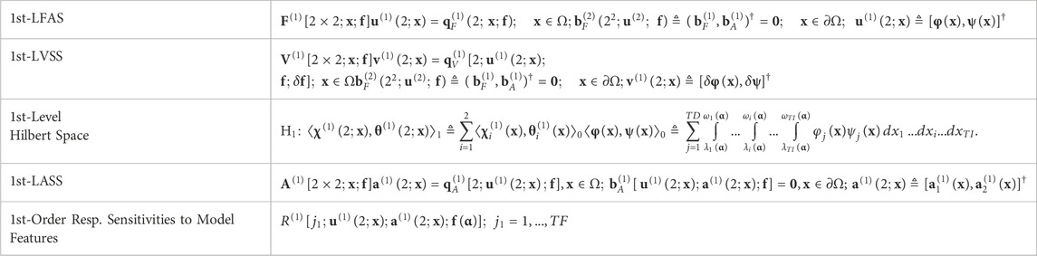
Table 1. 1st-FASAM-L: 1st-order (n = 1) sensitivities of response to model features.
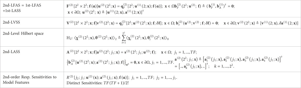
Table 2. 2nd-FASAM-L: 2nd-order (n = 2) sensitivities of response to model features.
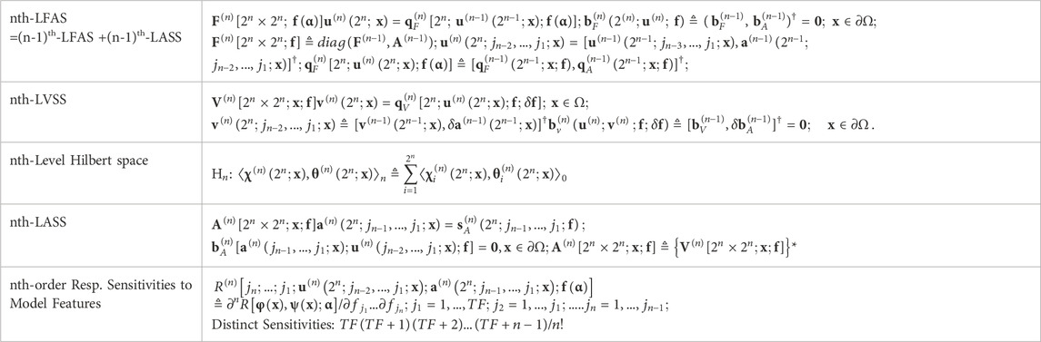
Table 3. nth-FASAM-L: nth-order sensitivities of response to model features.
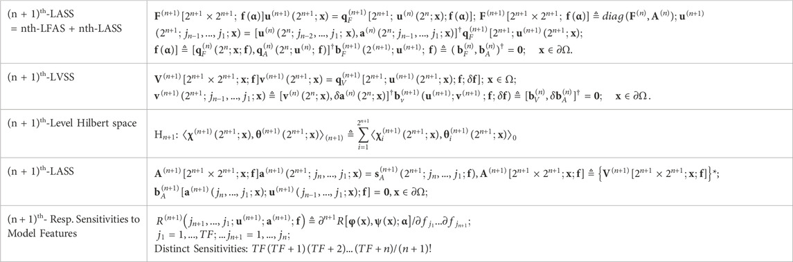
Table 4. (n + 1)th-FASAM-L: (n + 1)th-order sensitivities of response to model features.
An overview, in tabular form, of the computational frameworks of the nth-CASAM-L, nth-CASAM-N, nth-FASAM-L, and nth-FASAM-N methodologies, highlighting their objectives, characteristics, and interrelationships is presented in Table 5, below.
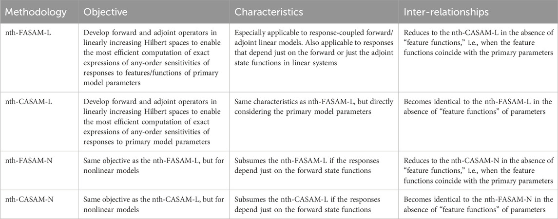
Table 5. The nth-CASAM-L, nth-CASAM-N, nth-FASAM-L, nth-FASAM-N methodologies: main features.
Formally, the results produced by the nth-FASAM-L can be written in the same mathematical forms as those produced by the nth-CASAM-L, with the fundamental difference that the number of large-scale computations needed within the nth-FASAM-L is dictated by the number
3 Concluding discussion
This work has presented the “nth-Order Feature Adjoint Sensitivity Analysis Methodology for Response-Coupled Forward/Adjoint Linear Systems” (abbreviated as “nth-FASAM-L”), which is the most efficient methodology for computing exact expressions of sensitivities of model responses to features of model parameters and, subsequently, to the model parameters themselves for such linear systems. This efficiency stems from the maximal reduction of the number of adjoint computations (which are “large-scale” computations), by comparison to the extant high-order adjoint sensitivity analysis methodology nth-CASAM-N (the “nth-Order Comprehensive Adjoint Sensitivity Analysis Methodology for Nonlinear Systems”). Specific details are as follows:
(i) Comparing the mathematical framework of the nth-FASAM-N methodology to the framework of the nth-CASAM-N methodology indicates that the components
(ii) The 1st-FASAM-N and the 1st-CASAM-N methodologies require a single large-scale “adjoint” computations for solving the 1st-LASS (1st-Level Adjoint Sensitivity System), so they are comparably efficient for computing the exact expressions of the first-order sensitivities of a model response to the model’s uncertain parameters, boundaries, and internal interfaces.
(iii) For computing the exact expressions of the second-order response sensitivities with respect to the primary model’s parameters, the 2nd-FASAM-N methodology requires, at most, as many large-scale “adjoint” computations as there are “feature functions of parameters”
(iv) For computing the exact expressions of the third-order response sensitivities with respect to the primary model’s parameters, the 3rd-FASAM-N requires at most
(v) When a model has no “feature” functions of parameters, but only comprises primary parameters, the nth-FASAM-N methodology becomes identical to the nth-CASAM-N methodology.
(vi) Both the nth-FASAM-N and the nth-CASAM-N methodologies are formulated in linearly increasing higher-dimensional Hilbert spaces −as opposed to exponentially increasing parameter-dimensional spaces− thus overcoming the curse of dimensionality in sensitivity analysis of nonlinear systems. Both the nth-FASAM-N and the nth-CASAM-N methodologies are incomparably more efficient and more accurate than any other methods (statistical, finite differences, etc.) for computing exact expressions of response sensitivities (of any order) with respect to the model’s uncertain parameters, boundaries, and internal interfaces.
The question of “when to stop computing progressively higher-order sensitivities ?” has been addressed by Cacuci (2022), Cacuci D. G. (2023) in conjunction with the question of convergence of the Taylor-series expansion of the response in terms of the uncertain model parameters, cf; Eqs 10, 12. These Taylor-series expansions provide the fundamental premise, even if not explicitly recognized, for obtaining the expressions provided by the “propagation of errors” methodology (as originally proposed by Tukey, 1957; and generalized by Cacuci, 2022) for the cumulants of the model response distribution in the phase-space of model parameters. The convergence of these Taylor-series, which depend on both the response sensitivities with respect to parameters and the uncertainties associated with the parameter distribution, must be ensured. This can be done by ensuring that the combination of parameter uncertainties and response sensitivities are sufficiently small to fall inside the respective radius of convergence of each of these Taylor-series expansions. The application of the nth-FASAM-N to a representative response-coupled forward/adjoint linear model stemming from the field of energy-dependent particle transport in a mixture of materials will be presented in the accompanying work designated as “Part II” (Cacuci, 2024c).
Data availability statement
The original contributions presented in the study are included in the article/supplementary material, further inquiries can be directed to the corresponding author.
Author contributions
DC: Conceptualization, Methodology, Project administration, Validation, Writing–original draft, Writing–review and editing.
Funding
The author(s) declare that no financial support was received for the research, authorship, and/or publication of this article.
Conflict of interest
The author declares that the research was conducted in the absence of any commercial or financial relationships that could be construed as a potential conflict of interest.
Publisher’s note
All claims expressed in this article are solely those of the authors and do not necessarily represent those of their affiliated organizations, or those of the publisher, the editors and the reviewers. Any product that may be evaluated in this article, or claim that may be made by its manufacturer, is not guaranteed or endorsed by the publisher.
References
Alcouffe, R. E., Baker, R. S., Dahl, J. A., Turner, S. A., and Ward, R. (2008). PARTISN: a time-dependent, parallel neutral particle transport code system. Los Alamos, NM, USA: Los Alamos National Laboratory. LA-UR-08-07258.
Bellman, R. E. (1957). Dynamic programming. USA: Rand Corporation, Princeton University Press. Republished: Bellman, RE (2003) Dynamic Programming. Courier Dover Publications, ISBN 978-0-486-42809-3, USA.
Cacuci, D. G. (1981). Sensitivity theory for nonlinear systems: I. Nonlinear functional analysis approach. J. Math. Phys. 22, 2794–2802. doi:10.1063/1.525186
Cacuci, D. G. (2015). Second-order adjoint sensitivity analysis methodology (2nd-ASAM) for computing exactly and efficiently first- and second-order sensitivities in large-scale linear systems: I. Computational methodology. J. Comp. Phys. 284, 687–699. doi:10.1016/j.jcp.2014.12.042
Cacuci, D. G. (2016). The second-order adjoint sensitivity analysis methodology for nonlinear systems—I: theory. Nucl. Sci. Eng. 184, 16–30. doi:10.13182/nse16-16
Cacuci, D. G. (2022). The nth-order comprehensive adjoint sensitivity analysis methodology (nth-CASAM): overcoming the curse of dimensionality in sensitivity and uncertainty analysis, Volume I: linear systems. Cham, Switzerland: Springer Nature, 362. doi:10.1007/978-3-030-96364-4
Cacuci, D. G. (2023a). The nth-order comprehensive adjoint sensitivity analysis methodology (nth-CASAM): overcoming the curse of dimensionality in sensitivity and uncertainty analysis, volume III: nonlinear systems. Cham, Switzerland: Springer Nature, 369. doi:10.1007/978-3-031-22757-8
Cacuci, D. G. (2023b). Computation of high-order sensitivities of model responses to model parameters. II: introducing the second-order adjoint sensitivity analysis methodology for computing response sensitivities to functions/features of parameters. Energies 16, 6356. doi:10.3390/en16176356
Cacuci, D. G. (2024a). Introducing the nth-order features adjoint sensitivity analysis methodology for nonlinear systems (nth-FASAM-N): I. Mathematical framework. Am. J. Comput. Math. 14, 11–42. doi:10.4236/ajcm.2024.141002
Cacuci, D. G. (2024b). Introducing the nth-order features adjoint sensitivity analysis methodology for nonlinear systems (nth-FASAM-N): II. Illustrative example. Am. J. Comput. Math. 14, 43–95. doi:10.4236/ajcm.2024.141003
Cacuci, D. G. (2024c). The nth-order features adjoint sensitivity analysis methodology for response-coupled forward/adjoint linear systems (nth-FASAM-L): I. mathematical framework. Front. Energy Res 12, 1417594. doi:10.3389/fenrg.2024.1417594
Cacuci, D. G., and Fang, R. (2023). The nth-order comprehensive adjoint sensitivity analysis methodology (nth-CASAM): overcoming the curse of dimensionality in sensitivity and uncertainty analysis, volume II: application to a large-scale system. Nature Switzerland, Cham: Springer, 463. doi:10.1007/978-3-031-19635-5
Chadwick, M. B., Herman, M., Obložinský, P., Dunn, M. E., Danon, Y., Kahler, A. C., et al. (2011). ENDF/B-VII.1: nuclear data for science and technology: cross sections, covariances, fission product yields and decay data. Nucl. Data Sheets 112, 2887–2996. doi:10.1016/j.nds.2011.11.002
Conlin, J. L., Parsons, D. K., Gardiner, S. J., Gray, M., Lee, M. B., and White, M. C. (2013). MENDF71X: multigroup neutron cross-section data tables based upon ENDF/B-VII.1X; los alamos national laboratory report LA-UR-15-29571. Los Alamos, NM, USA: Los Alamos National Laboratory, 2013.
Cukier, R. I., Levine, H. B., and Shuler, K. E. (1978). Nonlinear sensitivity analysis of multiparameter model systems. J. Comput. Phys. 26, 1–42. doi:10.1016/0021-9991(78)90097-9
Dunker, A. M. (1984). The decoupled direct method for calculating sensitivity coefficients in chemical kinetics. J. Chem. Phys. 81, 2385–2393. doi:10.1063/1.447938
Hora, S. C., and Iman, R. L. (1986). A Comparison of maximum/bounding and Bayesian/Monte Carlo for fault tree uncertainty analysis. Albuquerque, NM, USA: Sandia National Laboratories. Technical Report SAND85-2839.
Iman, R. L., Helton, J. C., and Campbell, J. E. (1981a). An approach to sensitivity analysis of computer models: Part I—introduction, input variable selection and preliminary variable assessment. J. Qual. Technol. 13, 174–183. doi:10.1080/00224065.1981.11978748
Iman, R. L., Helton, J. C., and Campbell, J. E. (1981b). An approach to sensitivity analysis of computer models: Part II—ranking of input variables, response surface validation, distribution effect and technique synopsis. J. Qual. Technol. 13, 232–240. doi:10.1080/00224065.1981.11978763
Kramer, M. A., Calo, J. M., and Rabitz, H. (1981). An improved computational method for sensitivity analysis: green’s Function Method with “AIM”. Appl. Math. Model. 5, 432–441. doi:10.1016/s0307-904x(81)80027-3
Luo, Z., Wang, X., and Liu, D. (2020). Prediction on the static response of structures with large-scale uncertain-but-bounded parameters based on the adjoint sensitivity analysis. Struct. Multidiscip. Optim. 61, 123–139. doi:10.1007/s00158-019-02349-w
Práger, T., and Kelemen, F. D. (2014). “Adjoint methods and their application in earth sciences,” in Advanced numerical methods for complex environmental models: needs and availability. Editors I. Faragó, Á. Havasi, and Z. Zlatev (Oak Park, IL, USA: Bentham Science Publishers), 203–275. Chapter 4A.
Rios Insua, D. (1990). Sensitivity analysis in multiobjective decision making. New York, USA: Springer Verlag.
Saltarelli, A., Chan, K., and Scott, E. M. (2000). Sensitivity analysis (Chichester, UK: J. Wiley and Sons Ltd).
Shultis, J. K., and Faw, R. E. (2000). Radiation shielding. La Grange Park, Illinois, USA: American Nuclear Society.
Tukey, J. W. (1957). The propagation of errors, fluctuations and tolerances. Princeton, NJ, USA: Princeton University. Technical Reports No. 10-12.
Valentine, T. E. (2006). Polyethylene-reflected plutonium metal sphere subcritical noise measurements, SUB-PU-METMIXED-001. International handbook of evaluated criticality safety benchmark experiments, NEA/NSC/DOC(95)03/I-IX, organization for economic Co-operation and development (OECD). Paris, France: Nuclear Energy Agency.
Weiberg, A. M., and Wigner, E. P. (1958). The physical theory of neutron chain reactors. Chicago, Illinois, USA: University of Chicago Press.
Weisbin, C. R., Oblow, E. M., Marable, J. H., Peelle, R. W., and Lucius, J. L. (1978). Application of sensitivity and uncertainty methodology to fast reactor integral experiment analysis. Nucl. Sci. Eng. 66, 307–333. doi:10.13182/nse78-3
Wigner, E. P. (1945). Effect of small perturbations on pile period. Chicago, IL, USA: Scientific Research Publishing. Chicago Report CP-G-3048.
Williams, M. L. (1986). “Perturbation theory for nuclear reactor analysis,” in Handbook of nuclear reactor calculations. Editor Y. Ronen (Boca Raton, Florida, USA: CRC Press), 63–188. Volume 3.
Williams, M. L., and Engle, W. W. (1977). The concept of spatial channel theory applied to reactor shielding analysis. Nucl. Sci. Eng. 62, 92–104. doi:10.13182/nse77-a26941
Wilson, W. B., Perry, R. T., Shores, E. F., Charlton, W. S., Parish, T. A., Estes, G. P., et al. (2002). “SOURCES4C: a code for calculating (α,n), spontaneous fission, and delayed neutron sources and spectra,” in Proceedings of the American Nuclear Society/Radiation Protection and Shielding Division 12th Biennial Topical Meeting, Santa Fe, NM, USA, 14–18 April 2002.
Keywords: response-coupled forward/adjoint model, features of model parameters, adjoint operators in Hilbert spaces, exact sensitivities of arbitrarily high order, most efficient computation of high order response sensitivities
Citation: Cacuci DG (2024) The nth-order features adjoint sensitivity analysis methodology for response-coupled forward/adjoint linear systems (nth-FASAM-L): I. mathematical framework. Front. Energy Res. 12:1417594. doi: 10.3389/fenrg.2024.1417594
Received: 15 April 2024; Accepted: 26 June 2024;
Published: 13 August 2024.
Edited by:
Yang Zou, Chinese Academy of Sciences (CAS), ChinaReviewed by:
Jian Guo, Chinese Academy of Sciences (CAS), ChinaShichang Liu, North China Electric Power University, China
Copyright © 2024 Cacuci. This is an open-access article distributed under the terms of the Creative Commons Attribution License (CC BY). The use, distribution or reproduction in other forums is permitted, provided the original author(s) and the copyright owner(s) are credited and that the original publication in this journal is cited, in accordance with accepted academic practice. No use, distribution or reproduction is permitted which does not comply with these terms.
*Correspondence: Dan Gabriel Cacuci, Y2FjdWNpQGNlYy5zYy5lZHU=