An L1-and-L2-regularized nonnegative tensor factorization for power load monitoring data imputation

As smart grid advance, Power Load Forecasting (PLF) has become a research hotspot. As the foundation of the forecasting model, the Power Load Monitoring (PLM) data takes on great importance due to its completeness, reliability and accuracy. However, monitoring equipment failures, transmission channel congestion and anomalies result in missing PLM data, which directly affects the performance of the PLF model. To address this issue, this paper proposes an L₁-and-L₂-Regularized Nonnegative Tensor Factorization (LNTF) model to impute PLM missing data. Its main idea is threefold: (1) combining L₁ and L₂ norms to achieve effective feature extraction and improve the model’s robustness; (2) incorporating two temporal-dependent linear biases to describe the fluctuations of PLM data; (3) adding nonnegative constraints to precisely define the nonnegativity of PLM data. Extensive empirical studies on two publicly real-world PLM datasets with 1,569,491 and 413,357 known entries and missing rates of 93.35% and 96.75% demonstrate that the proposed LNTF improves 14.04%, 59.31%, and 71.43% on average over the state-of-the-art imputation models in terms of imputation error, convergence rounds, and time cos, respectively. Its high computational efficiency and low imputation error make practical sense for PLM data imputation.

1 Introduction

As one of the most commonly utilized technologies in the electric power industry, the Power Load Forecasting (PLF) (Chakhchoukh et al., 2010; Borges et al., 2012; Zhang et al., 2022; Yang Y. et al., 2023; Wang et al., 2024) is critical to the operation and planning for the power systems, which helps power companies make reasonable decisions to improve the stability and efficiency of the electric grid (Hafeez et al., 2020; Hammad et al., 2020; Li et al., 2021; Duan et al., 2023; Shirkhani et al., 2023). On the other hand, the Power Load Monitoring (PLM) (Tabatabaei et al., 2016; Abubakar et al., 2017; Wang et al., 2023) observes and records various parameters in the power systems, thereby effectively monitoring the power load situation (Zhang et al., 2023; Shao et al., 2023; D’Incecco et al., 2019; Song et al., 2022), and it provides an extensive data foundation for PLF models. However, there are missing PLM data due to sensor failures, network failures, and transmission delays (Wang et al., 2021). In addition, since PLM data needs to be collected frequently, its data scale is large. Therefore, the PLM data is High Dimensional and Incomplete (HDI) (Hu et al., 2020; Luo et al., 2021a; Wu and Luo, 2021; Wu et al., 2023a; Wu et al., 2023b).

Although the existing imputation models are able to complete the imputation of missing PLM data, but their computational and time overheads are expensive and they do not consider the simultaneous missing of multiple monitoring parameters. In contrast, the PLM data collects various monitoring parameters such as electric current, electric voltage, and electric power. On the other hand, temporal variations significantly affect model performance. Since PLM data have temporal characteristics, such as the difference between daytime and nighttime loads, different weekday and weekend usage patterns, and seasonal variations in summer and winter, the static model cannot accurately predict the load variations. Therefore, it is essential to implement a temporal variation-incorporated imputation model that can be applied to multiple monitoring parameters with efficient computation and fast response on HDI PLM data (Wu et al., 2019; Chen J. et al., 2021; Hu et al., 2021; Li Z. et al., 2022; Wu et al., 2022a; Wu et al., 2022b).

By previous studies (Nie et al., 2016; Luo et al., 2019a; Wu et al., 2020; Wu et al., 2021a; Chen K. et al., 2021; Luo et al., 2021b; Zhao et al., 2021; Qin et al., 2023), Tensor Factorization (TF)-based imputation methods are able to efficiently impute missing data by constructing the data as a higher-order tensor. Specifically, based on the Canonical Polyadic Decomposition (CPD) (Wu et al., 2021b), the TF-based model decomposes the higher-order tensor into an outer product of multiple Factor Matrices (FM) to provide a concise and unique representation (Bulat et al., 2020). For instance, Wu et al. (2021a) proposed a Proportional-Integral-Derivative (PID) TF-based model to impute missing data, which adopts the PID control principle to construct the tuning instance error, and optimizes the model parameters by the Stochastic Gradient Descent (SGD) algorithm to achieve a lower imputation error. Wang et al. (2019) incorporated a momentum term into the solving process of SGD based on CPD to accelerate the convergence process. Moreover, the TF-based models can naturally incorporate nonnegative constraints to deal with the data with nonnegativity, called Nonnegative Tensor Factorization (NTF) models (Qin et al., 2022; Xu et al., 2023; Chen et al., 2024). Luo et al. (2022) proposed an NTF model incorporating the neural dynamics principle, which constructs the CPD process as a neural network layer and introduces nonlinearity through the activation functions, thereby achieving efficient imputation of missing data. Che et al. (2023) proposed a sparse and graph regularization TF-based model for fake news detection, which employs a monotonically non-increasing algorithm to solve the model efficiently and obtain excellent model performance.

Therefore, this paper proposes an L₁-and-L₂-regularized-based Nonnegative Tensor-factorization (LNTF) model to impute missing PLM data. It employs a tensor to model PLM data with temporal features. Specifically, during 1 day, we arrange the sampling frequency by time and it preserves the temporal pattern of the monitored parameters. In addition, the cyclical structure of the data is further preserved by arranging the monitoring parameters of each day by time. As a result, the temporal dynamics of the data is fully reflected in the constructed three-order tensor. It further incorporates temporal-dependent linear biases to address the fluctuations of PLM data. Finally, it combines L₁ and L₂ regularizations to improve the generalization ability and robustness of the model, thereby achieve an efficient model with low imputation error and fast convergence. The main contributions of this paper are presented as follows:

1) A three-order tensor construction. It fully preserves the temporal pattern of PML data.

2) An LNTF model. It provides highly accurate imputation for missing PLM data.

3) An effective LNTF learning scheme. ItschI guarantees the non-negativity of PML data.

Experimental results on two publicly available datasets indicate that the LNTF model is superior to the existing imputation models for PLM data in terms of imputation error, convergence rounds, and time cost.

Section 2 presents the related works, Section 3 gives the Preliminaries, and Section 4 introduces the proposed LNTF model in detail. Section 5 shows the comparative experiments. The conclusions and future work are provided in Section 6.

2 Related works

For data imputation, common methods such as Lagrange interpolation (Allik and Annuk, 2017) and the K-nearest neighbors method (Miao et al., 2016) are often employed. However, these methods perform poorly in scenarios with high missing rates. Liu et al. (2012) defined tensor nuclear norm as the combination of matrix nuclear norms obtained by unfolding the tensor along its modes. Yang and Nagarajaiah (2016) utilized prior knowledge of data structure to minimize the nuclear norm and complete low-rank matrices. Gao et al. (2017) designed a subspace merging method to represent real-world datasets by merging multiple subspaces into a larger one for missing data imputation. However, converting a third-order tensor into matrices loses the original multi-dimensional structural information. Kilmer and Martin (2011) proposed the tensor singular value decomposition method, which demonstrates the multi-dimensional structure by constructing a group ring along the tensor fibers, effectively capturing the inherent low-rank structure of the tensor. He et al. (2019) proposed a Kalman filter model that derives a recursive analytical solution and uses the least squares method to estimate the missing data. To date, researchers have proposed various data imputation models for missing PLM data. Alamoodi et al. (2021) proposed a deep learning-based imputation model for incomplete data, which captures the spatial-temporal relationships of the data through deep learning models and completes the imputation of missing data. Amritkar and Kumar (1995) constructed an encoder-decoder model to impute missing data employing long-short-term memory networks and graph convolution principles. Yang T. et al. (2023) proposed a missing data imputation model based on an improved generative adversarial network, which adopts a deep network model to extract the spatial-temporal correlation of data to achieve better imputation performance. Zhang et al. (2020) proposed a relational graph neural network with a hierarchical attention mechanism, which effectively exploits neighborhood information to highlight the importance of different entities, thereby completing accurately the missing data imputation. Luo et al. (2023) proposed a graph neural network based on attention relation paths, and introduced a neural process based on normalized flow to improve the performance of imputation. Nevertheless, these models generating the entire tensor and calculating the singular values of matrices or tensors, leading to low computational efficiency and excessively high memory requirements.

3 Preliminaries

3.1 Symbol appointment

The symbol system adopted in this paper is presented in Table 1.

Table 1

Table 1. Adopted symbols and their descriptions.

3.2 Problem formulation

Figure 1 presents the process of modeling PLM data to an HDI tensor. Specifically, a set of monitoring parameter data first forms a parameter vector. Then a frequency-parameter matrix is constituted by multiple samples per day. Finally, multiple frequency-parameter matrices are stacked along the temporal dimension to construct a third-order tensor.

Figure 1

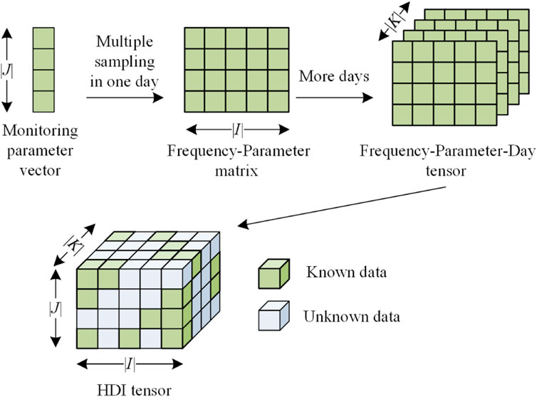
Figure 1. An HDI tensor from PLM data.

Definition 1. (Three-order HDI frequency-parameter-day tensor): Given a parameter-frequency-day tensor Y^{|I|×|J|×|K|}, where each element y_ijk denotes the ith (i∈I) parameter information in the jth (j∈J) sampling point of kth (k∈K) day. Λ and Γ denote the known and unknown data, respectively. Y is an HDI tensor if |Λ|≪|Γ|.

Based on previous research (Luo et al., 2017; Luo et al., 2021c), this paper follows the principle of CPD to implement TF process as shown in Figure 2.

$\mathbf{X}={\displaystyle \sum _{r=1}^R}{\mathbf{H}}_r.(1)$

With (1), an HDI tensor can be decomposed to R rank-one tensors.

Figure 2

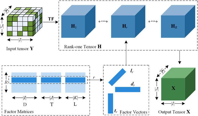
Figure 2. Latent factorization of an HDI tensor Y.

Definition 2. (Rank-one tensor): Given a rank-one tensor H^{|I|×|J|×|K|} _r, it can be written as the outer product of three factor vectors H_r = d_r°t_r°l_r, where d_r, t_r, and l_r are the r-th rows of the factor matrices D^|I|×|R|, T^|J|×|R|, and L^|K|×|R|, respectively.

Thus, by unfolding the rank-one tensor, each element x_ijk in X is expressed by (Eq. 2):

${\mathit{x}}_{\mathit{i}\mathit{j}\mathit{k}}={\displaystyle \sum _{\mathit{r}=\mathbf{1}}^{\mathit{R}}}{\mathit{h}}_{\mathit{i}\mathit{j}\mathit{k}}^{\left(\mathit{r}\right)}={\displaystyle \sum _{\mathit{r}=\mathbf{1}}^{\mathit{R}}}{\mathit{d}}_{\mathit{i}\mathit{r}}{\mathit{t}}_{\mathit{j}\mathit{r}}{\mathit{l}}_{\mathit{k}\mathit{r}}.(2)$

To obtain the desired three FMs, we depend on the Euclidean distance (Wang et al., 2005; Shang et al., 2021) to construct an objective function ε, it’s given as (Eq. 3):

$\mathit{\epsilon }=\frac{\mathbf{1}}{\mathbf{2}}{‖\mathbf{Y}-\mathbf{X}‖}_{\mathit{F}}^{\mathbf{2}}(3)$

Note that numerous entries in Y are unknown, and we define ε on known entries Λ to accurately characterize the difference between the original element y_ijk and the reformulated element x_ijk as (Eq. 4) (Luo et al., 2015; Luo et al., 2019b):

$\mathit{\epsilon }=\frac{\mathbf{1}}{\mathbf{2}}{\displaystyle \sum _{{\mathit{y}}_{\mathit{i}\mathit{j}\mathit{k}}\in \mathbf{\Lambda }}}{\left({\mathit{y}}_{\mathit{i}\mathit{j}\mathit{k}}-{\mathit{x}}_{\mathit{i}\mathit{j}\mathit{k}}\right)}^{\mathbf{2}}=\frac{\mathbf{1}}{\mathbf{2}}{\displaystyle \sum _{{\mathit{y}}_{\mathit{i}\mathit{j}\mathit{k}}\in \mathbf{\Lambda }}}{\left({\mathit{y}}_{\mathit{i}\mathit{j}\mathit{k}}-{\displaystyle \sum _{\mathit{r}=\mathbf{1}}^{\mathit{R}}}{\mathit{d}}_{\mathit{i}\mathit{r}}{\mathit{t}}_{\mathit{j}\mathit{r}}{\mathit{l}}_{\mathit{k}\mathit{r}}\right)}^{\mathbf{2}}(4)$

Normally, the PLM data is nonnegative and it is necessary to add nonnegative constraints for FMs to correctly describe the data’s nonnegativity. Therefore, the objective function of the NTF is formulated as (Eq. 5):

$\begin{array}{l}\mathit{\epsilon }=\frac{\mathbf{1}}{\mathbf{2}}{\displaystyle \sum _{{\mathit{y}}_{\mathit{i}\mathit{j}\mathit{k}}\in \mathbf{\Lambda }}}{\left({\mathit{y}}_{\mathit{i}\mathit{j}\mathit{k}}-{\mathit{x}}_{\mathit{i}\mathit{j}\mathit{k}}\right)}^{\mathbf{2}}=\frac{\mathbf{1}}{\mathbf{2}}{\displaystyle \sum _{{\mathit{y}}_{\mathit{i}\mathit{j}\mathit{k}}\in \mathbf{\Lambda }}}{\left({\mathit{y}}_{\mathit{i}\mathit{j}\mathit{k}}-{\displaystyle \sum _{\mathit{r}=\mathbf{1}}^{\mathit{R}}}{\mathit{d}}_{\mathit{i}\mathit{r}}{\mathit{t}}_{\mathit{j}\mathit{r}}{\mathit{l}}_{\mathit{k}\mathit{r}}\right)}^{\mathbf{2}}\\ \mathbf{s}.\mathbf{t}.\forall \mathit{i}\in \mathit{I},\forall \mathit{j}\in \mathit{J},\forall \mathit{k}\in \mathit{K},\forall \mathit{r}\in \left\{1\sim R\right\}:{\mathit{d}}_{\mathit{i}\mathit{r}}\ge 0,{\mathit{t}}_{\mathit{j}\mathit{r}}\ge 0,{\mathit{l}}_{\mathit{k}\mathit{r}}\ge 0.\end{array}(5)$

4 LNTF model

4.1 Objective function

For the HDI PLM tensor, the monitoring parameter data fluctuate with sampling frequency and time. According to previous research (Li et al., 2016; Yuan et al., 2018), it is essential to incorporate the linear bias (LB) into the model to improve the performance when analyzing fluctuating data. Note that the constructed HDI PLM tensor has time-varying characteristics in I-dimension and K-dimension, we incorporate the corresponding two temporal-dependent LBs into the reformulated element x_ijk as (Eq. 6):

${\mathit{x}}_{\mathit{i}\mathit{j}\mathit{k}}={\displaystyle \sum _{\mathit{r}=\mathbf{1}}^{\mathit{R}}}{\mathit{d}}_{\mathit{i}\mathit{r}}{\mathit{t}}_{\mathit{j}\mathit{r}}{\mathit{l}}_{\mathit{k}\mathit{r}}+{\mathit{p}}_{\mathit{i}}+{\mathit{q}}_{\mathit{k}}.(6)$

To deal with the unbalanced distribution of known entries and to avoid overfitting the model, it is necessary to incorporate regularization terms in the objective function (Luo et al., 2019c; Liu et al., 2023). Typically, L₁-regularized makes the FMs sparse during the optimization process, which is effective for selecting features since it automatically removes insignificant features. However, incorporating L₁-regularized results in a non-smooth objective function (Grasmair et al., 2011; Wu D. et al., 2021). On the other hand, L₂-regularized tends to optimize the FMs uniformly by narrowing the feature values and improving the robustness of the model, but it is sensitive towards outliers (Zeng et al., 2017; Jin et al., 2019; Benjamin and Yang, 2021). Hence, we assemble the L₁-regularized and L₂-regularized to combine their advantages, while adopting an approximation to deal with the absolute value in L₁-regularized to make the objective function smooth. Further, the objective function is formulated as (Eq. 7):

$\begin{array}{l}\mathit{\epsilon }=\frac{\mathbf{1}}{\mathbf{2}}{\displaystyle \sum _{{\mathit{y}}_{\mathit{i}\mathit{j}\mathit{k}}\in \mathbf{\Lambda }}}\left({\left({\mathit{y}}_{\mathit{i}\mathit{j}\mathit{k}}-{\displaystyle \sum _{\mathit{r}=\mathbf{1}}^{\mathit{R}}}{\mathit{d}}_{\mathit{i}\mathit{r}}{\mathit{t}}_{\mathit{j}\mathit{r}}{\mathit{l}}_{\mathit{k}\mathit{r}}-{\mathit{p}}_{\mathit{i}}-{\mathit{q}}_{\mathit{k}}\right)}^{\mathbf{2}}\right)\\ +\frac{\mathbf{1}}{\mathbf{2}}{\displaystyle \sum _{{\mathit{y}}_{\mathit{i}\mathit{j}\mathit{k}}\in \mathbf{\Lambda }}}\left(\mathit{\lambda }\left({\displaystyle \sum _{\mathit{r}=\mathbf{1}}^{\mathit{R}}}\left({\mathit{d}}_{\mathit{i}\mathit{r}}^{\mathbf{2}}+\sqrt{{\mathit{d}}_{\mathit{i}\mathit{r}}^{\mathbf{2}}+\mathit{\tau }}+{\mathit{t}}_{\mathit{j}\mathit{r}}^{\mathbf{2}}+\sqrt{{\mathit{t}}_{\mathit{j}\mathit{r}}^{\mathbf{2}}+\mathit{\tau }}+{\mathit{l}}_{\mathit{k}\mathit{r}}^{\mathbf{2}}+\sqrt{{\mathit{l}}_{\mathit{k}\mathit{r}}^{\mathbf{2}}+\mathit{\tau }}\right)\right)\right)\\ +\frac{\mathbf{1}}{\mathbf{2}}{\displaystyle \sum _{{\mathit{y}}_{\mathit{i}\mathit{j}\mathit{k}}\in \mathbf{\Lambda }}}\left({\mathit{\lambda }}_{\mathit{b}}\left({\mathit{p}}_{\mathit{i}}^{\mathbf{2}}+\sqrt{{\mathit{p}}_{\mathit{i}}^{\mathbf{2}}+\mathit{\tau }}+{\mathit{q}}_{\mathit{k}}^{\mathbf{2}}+\sqrt{{\mathit{q}}_{\mathit{k}}^{\mathbf{2}}+\mathit{\tau }}\right)\right),\\ \mathbf{s}.\mathbf{t}.\forall \mathit{i}\in \mathit{I},\forall \mathit{j}\in \mathit{J},\forall \mathit{k}\in \mathit{K},\forall \mathit{r}\in \left\{1\sim R\right\}:d_{ir}\ge 0,t_{jr}\ge 0,l_{kr}\ge 0,p_i\ge 0,q_k\ge 0.\end{array}(7)$

where λ and λ_b are the regularized constants for FMs and LBs, respectively, and τ is a tiny positive number.

4.2 Learning scheme

Considering the nonnegativity of PLM data, we implement the NMU for FMs and LBs based on previous studies (Badeau et al., 2010; Liu et al., 2020). Specifically, additive gradient descent (AGD) is applied to (7) to implement the following learning rule:

$\begin{array}{l}\underset{\mathbf{D},\mathbf{T},\mathbf{L},\mathit{p},\mathit{q}}{\mathbf{argmin}}\mathit{\epsilon }\stackrel{\mathbf{\text{AGD}}}{\Rightarrow }\forall \mathit{i}\in \mathit{I},\mathit{j}\in \mathit{J},\mathit{k}\in \mathit{K},\mathit{r}\in \left\{\mathbf{1},\mathbf{2},...,\mathit{R}\right\}:\\ \left\{\begin{array}{l}{\mathit{d}}_{\mathit{i}\mathit{r}}\leftarrow {\mathit{d}}_{\mathit{i}\mathit{r}}-{\mathit{\eta }}_{\mathit{i}\mathit{r}}\frac{\partial \mathit{\epsilon }}{\partial {\mathit{d}}_{\mathit{i}\mathit{r}}}={\mathit{d}}_{\mathit{i}\mathit{r}}-{\mathit{\eta }}_{\mathit{i}\mathit{r}}\left({\displaystyle \sum _{{\mathit{y}}_{\mathit{i}\mathit{j}\mathit{k}}\in {\mathbf{\Lambda }}_{\left(\mathit{i}\right)}}}\left(\left({\mathit{y}}_{\mathit{i}\mathit{j}\mathit{k}}-{\mathit{x}}_{\mathit{i}\mathit{j}\mathit{k}}\right)\left(-{\mathit{t}}_{\mathit{j}\mathit{r}}{\mathit{l}}_{\mathit{k}\mathit{r}}\right)+\mathit{\lambda }\left({\mathit{d}}_{\mathit{i}\mathit{r}}+\frac{{\mathit{d}}_{\mathit{i}\mathit{r}}}{\sqrt{{\mathit{d}}_{\mathit{i}\mathit{r}}^{\mathbf{2}}+\mathit{\tau }}}\right)\right)\right)\\ {\mathit{p}}_{\mathit{i}}\leftarrow {\mathit{p}}_{\mathit{i}}-{\mathit{\eta }}_{\mathit{i}}\frac{\partial \mathit{\epsilon }}{\partial {\mathit{p}}_{\mathit{i}}}={\mathit{p}}_{\mathit{i}}-{\mathit{\eta }}_{\mathit{i}}\left({\displaystyle \sum _{{\mathit{y}}_{\mathit{i}\mathit{j}\mathit{k}}\in {\mathbf{\Lambda }}_{\left(\mathit{i}\right)}}}\left(\left(-{\mathit{y}}_{\mathit{i}\mathit{j}\mathit{k}}+{\mathit{x}}_{\mathit{i}\mathit{j}\mathit{k}}\right)+{\mathit{\lambda }}_{\mathit{b}}\left({\mathit{p}}_{\mathit{i}}+\frac{{\mathit{p}}_{\mathit{i}}}{\sqrt{{\mathit{p}}_{\mathit{i}}^{\mathbf{2}}+\mathit{\tau }}}\right)\right)\right),\end{array}\right.\end{array}(8)$

where η_ij and η_i denote the learning rates for d_ir and p_i, respectively. Note that we only present the update rules for one FM and one LB, since similar inferences are applied to {t_jr, l_kr} and q_k. Further, we separate the positive and negative components in learning rule as:

$\left\{\begin{array}{l}{\mathit{d}}_{\mathit{i}\mathit{r}}\leftarrow {\mathit{d}}_{\mathit{i}\mathit{r}}+{\mathit{\eta }}_{\mathit{i}\mathit{r}}\left({\displaystyle \sum _{{\mathit{y}}_{\mathit{i}\mathit{j}\mathit{k}}\in {\mathbf{\Lambda }}_{\left(\mathit{i}\right)}}}{\mathit{y}}_{\mathit{i}\mathit{j}\mathit{k}}{\mathit{t}}_{\mathit{j}\mathit{r}}{\mathit{l}}_{\mathit{k}\mathit{r}}\right)-{\mathit{\eta }}_{\mathit{i}\mathit{r}}{\displaystyle \sum _{{\mathit{y}}_{\mathit{i}\mathit{j}\mathit{k}}\in {\mathbf{\Lambda }}_{\left(\mathit{i}\right)}}}\left(\left({\mathit{x}}_{\mathit{i}\mathit{j}\mathit{k}}{\mathit{t}}_{\mathit{j}\mathit{r}}{\mathit{l}}_{\mathit{k}\mathit{r}}\right)+\mathit{\lambda }\left({\mathit{d}}_{\mathit{i}\mathit{r}}+\frac{{\mathit{d}}_{\mathit{i}\mathit{r}}}{\sqrt{{\mathit{d}}_{\mathit{i}\mathit{r}}^{\mathbf{2}}+\mathit{\tau }}}\right)\right)\\ {\mathit{p}}_{\mathit{i}}\leftarrow {\mathit{p}}_{\mathit{i}}+{\mathit{\eta }}_{\mathit{i}}{\displaystyle \sum _{{\mathit{y}}_{\mathit{i}\mathit{j}\mathit{k}}\in {\mathbf{\Lambda }}_{\left(\mathit{i}\right)}}}{\mathit{y}}_{\mathit{i}\mathit{j}\mathit{k}}-{\mathit{\eta }}_{\mathit{i}}{\displaystyle \sum _{{\mathit{y}}_{\mathit{i}\mathit{j}\mathit{k}}\in {\mathbf{\Lambda }}_{\left(\mathit{i}\right)}}}\left({\mathit{x}}_{\mathit{i}\mathit{j}\mathit{k}}+{\mathit{\lambda }}_{\mathit{b}}\left({\mathit{p}}_{\mathit{i}}+\frac{{\mathit{p}}_{\mathit{i}}}{\sqrt{{\mathit{p}}_{\mathit{i}}^{\mathbf{2}}+\mathit{\tau }}}\right)\right).\end{array}\right.(9)$

In order to cancel the negative component in (8), the learning rates are adjusted as follows:

$\left\{\begin{array}{l}{\mathit{\eta }}_{\mathit{i}\mathit{r}}={\mathit{d}}_{\mathit{i}\mathit{r}}/{\displaystyle \sum _{{\mathit{y}}_{\mathit{i}\mathit{j}\mathit{k}}\in {\mathbf{\Lambda }}_{\left(\mathit{i}\right)}}}\left(\left({\mathit{x}}_{\mathit{i}\mathit{j}\mathit{k}}{\mathit{t}}_{\mathit{j}\mathit{r}}{\mathit{l}}_{\mathit{k}\mathit{r}}\right)+\mathit{\lambda }\left({\mathit{d}}_{\mathit{i}\mathit{r}}+\frac{{\mathit{d}}_{\mathit{i}\mathit{r}}}{\sqrt{{\mathit{u}}_{\mathit{i}\mathit{r}}^{\mathbf{2}}+\mathit{\tau }}}\right)\right)\\ {\mathit{\eta }}_{\mathit{i}}={\mathit{p}}_{\mathit{i}}/{\displaystyle \sum _{{\mathit{y}}_{\mathit{i}\mathit{j}\mathit{k}}\in {\mathbf{\Lambda }}_{\left(\mathit{i}\right)}}}\left({\mathit{x}}_{\mathit{i}\mathit{j}\mathit{k}}+{\mathit{\lambda }}_{\mathit{b}}\left({\mathit{p}}_{\mathit{i}}+\frac{{\mathit{p}}_{\mathit{i}}}{\sqrt{{\mathit{p}}_{\mathit{i}}^{\mathbf{2}}+\mathit{\tau }}}\right)\right).\end{array}\right.(10)$

With (9), (10), we obtain the multiplicative update rules for FMs and LBs as:

$\begin{array}{l}\underset{\mathbf{D},\mathbf{T},\mathbf{L},\mathit{p},\mathit{q}}{\mathbf{argmin}}\mathit{\epsilon }\stackrel{\mathbf{\text{AGD}}}{\Rightarrow }\forall \mathit{i}\in \mathit{I},\mathit{j}\in \mathit{J},\mathit{k}\in \mathit{K},\mathit{r}\in \left\{\mathbf{1},\mathbf{2},...,\mathit{R}\right\}:\\ \left\{\begin{array}{l}{\mathit{d}}_{\mathit{i}\mathit{r}}\leftarrow {\mathit{d}}_{\mathit{i}\mathit{r}}\left(\left({\displaystyle \sum _{{\mathit{y}}_{\mathit{i}\mathit{j}\mathit{k}}\in {\mathbf{\Lambda }}_{\left(\mathit{i}\right)}}}{\mathit{y}}_{\mathit{i}\mathit{j}\mathit{k}}{\mathit{t}}_{\mathit{j}\mathit{r}}{\mathit{l}}_{\mathit{k}\mathit{r}}\right)/{\displaystyle \sum _{{\mathit{y}}_{\mathit{i}\mathit{j}\mathit{k}}\in {\mathbf{\Lambda }}_{\left(\mathit{i}\right)}}}\left(\left({\mathit{x}}_{\mathit{i}\mathit{j}\mathit{k}}{\mathit{t}}_{\mathit{j}\mathit{r}}{\mathit{l}}_{\mathit{k}\mathit{r}}\right)+\mathit{\lambda }\left({\mathit{d}}_{\mathit{i}\mathit{r}}+\frac{{\mathit{d}}_{\mathit{i}\mathit{r}}}{\sqrt{{\mathit{d}}_{\mathit{i}\mathit{r}}^{\mathbf{2}}+\mathit{\tau }}}\right)\right)\right)\\ {\mathit{p}}_{\mathit{i}}\leftarrow {\mathit{p}}_{\mathit{i}}\left({\displaystyle \sum _{{\mathit{y}}_{\mathit{i}\mathit{j}\mathit{k}}\in {\mathbf{\Lambda }}_{\left(\mathit{i}\right)}}}{\mathit{y}}_{\mathit{i}\mathit{j}\mathit{k}}/{\displaystyle \sum _{{\mathit{y}}_{\mathit{i}\mathit{j}\mathit{k}}\in {\mathbf{\Lambda }}_{\left(\mathit{i}\right)}}}\left({\mathit{x}}_{\mathit{i}\mathit{j}\mathit{k}}+{\mathit{\lambda }}_{\mathit{b}}\left({\mathit{p}}_{\mathit{i}}+\frac{{\mathit{p}}_{\mathit{i}}}{\sqrt{{\mathit{p}}_{\mathit{i}}^{\mathbf{2}}+\mathit{\tau }}}\right)\right)\right).\end{array}\right.\end{array}(11)$

With (11), if D, T, L, p, and q are initially nonnegative, they maintain their nonnegativity during the update process.

4.3 Algorithm design and analysis

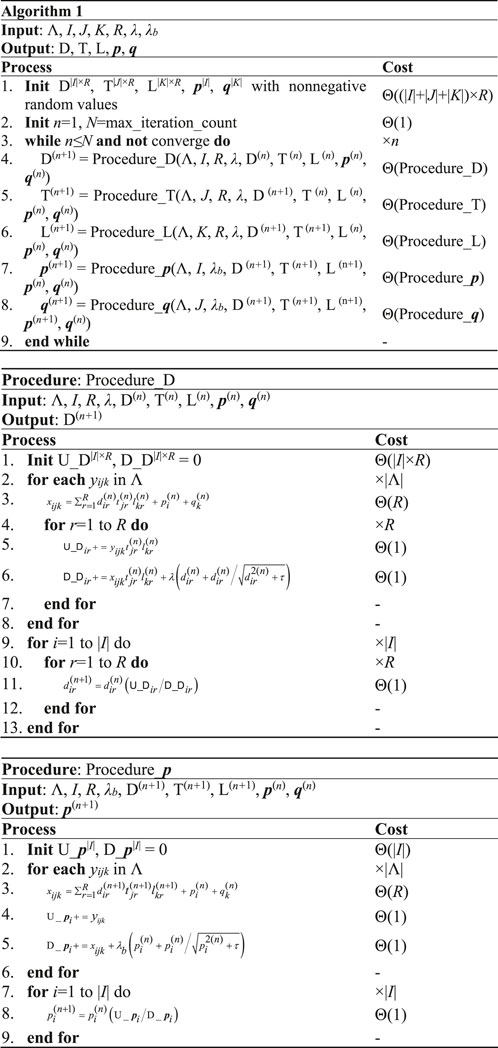
Based on the above inferences, we design the LNTF model as shown in Algorithm 1. Note that the pseudocodes of procedures {Procedure_D, Procedure_T, Procedure_L} and {Procedure_p, Procedure_q} in LNTF are similar, and we provide the update procedure for U and p as presented in Procedure_D and Procedure_p.

With Algorithm 1, the computational complexity of the LNTF model depends on the complexity of initializing and updating the FMs and LBs. Specifically, the computational complexity of procedure Update_D is presented as (Eq. 12):

${\mathit{C}}_{\mathbf{U}}=\mathrm{\Theta }\left(3R\times \left|\Lambda \right|+\mathbf{2}R\times \left|I\right|\right).(12)$

Similarly, the computational complexity of procedure Update_ p is given as (Eq. 13):

${\mathit{C}}_{\mathit{p}}=\mathrm{\Theta }\left(\left(2+R\right)\times \left|\Lambda \right|+2\left|I\right|\right).(13)$

Therefore, the computational complexity of LNTF model is:

$\begin{array}{l}{C}_{\text{LBNL}}=\Theta \left(R\times \left(\left|I\right|+\left|J\right|+\left|K\right|\right)+1+n\times \left(9R\times \left|\Lambda \right|+2R\times \left(\left|I\right|+\left|J\right|+\left|K\right|\right)+\left(\left(2+R\right)\times 2\left|\Lambda \right|+2\left|I\right|+2\left|K\right|\right)\right)\right)\\ \approx \Theta \left(n\times R\times \left|\Lambda \right|\right).\end{array}(14)$

Note that in (14), we omit the constant coefficients and lower order terms since |Λ| ≫ max{|I|, |J|, |K|} for an HDI tensor. With (14), n and R are positive constants in practical application, thus the computational complexity of the LNTF model is linear with the number of known entities in the HDI tensor.

For the storage complexity of the LNTF model, which depends on the number of known entities, the caches of FMs and LBs, the auxiliary matrices and arrays in the update procedures. Therefore, the storage complexity of the LNTF model is:

${\mathit{S}}_{\mathbf{\text{LBNL}}}=\mathbf{\Theta }\left(\left|\mathbf{\Lambda }\right|+\mathbf{2}\mathit{R}\times \left(\left|\mathit{I}\right|+\left|\mathit{J}\right|+\left|\mathit{K}\right|\right)+\mathbf{1}\right)\approx \mathbf{\Theta }\left(\left|\mathbf{\Lambda }\right|+\mathit{R}\times \left(\left|\mathit{I}\right|+\left|\mathit{J}\right|+\left|\mathit{K}\right|\right)\right).(15)$

With (15), constant constants and lower order terms are omitted, and the storage complexity of the LNTF model is linearly related to the number of known entities in the HDI tensor.

5 Empirical studies

5.1 General settings

In this section, all the comparison experiments are run on a desktop computer equipped with a 2.10 GHz Intel Core i7-13700 and a NVIDIA GeForce RTX 3050 GPU card. The versions of Java and Python used are SE-8U212 and Python 3.6.5, respectively.

5.1.1 Datasets

In this paper, two public PLM datasets iawe (Batra et al., 2013) and ukdale (Kelly and Knottenbelt, 2015) are used to compare model performance. They record load monitoring data of multiple appliances in the users’ homes, and the details are shown in Table 2. In D1, the monitoring parameters 13 parameters such as electric current, electric voltage, and electric power, etc., which are sampled 86,400 times per day for 21 days, and the number of known entries is 1,569,491. Note that we further split the datasets proportionally into disjoint training (Φ), validation (Ψ), and test sets (Ω) to evaluate the model performance, as shown in Table 3. In addition, we generate 20 random splits on each dataset to achieve unbiased model results.

Table 2

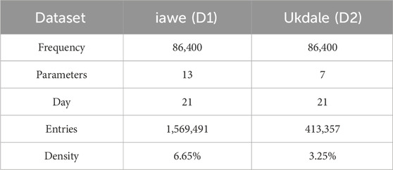
Table 2. Dataset details.

Table 3

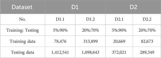
Table 3. Details settings of training datasets.

5.1.2 Evaluation metrics

The prediction accuracy in a given HDI PLM tensor directly reflects the prediction performance of the model. Based on previous studies (Li W. et al., 2022; Yuan et al., 2022; Bi et al., 2023; Wu et al., 2023c; Qin and Luo, 2023), Root mean squared error (RMSE) and mean absolute error (MAE) are commonly adopted as evaluation metrics for prediction accuracy, and they are given as (Eq. 16):

$\text{RMSE}=\sqrt{\frac{{\displaystyle \sum _{{\mathit{y}}_{\mathit{i}\mathit{j}\mathit{k}}\in \mathbf{\Omega }}}{\left({\mathit{y}}_{\mathit{i}\mathit{j}\mathit{k}}-{\mathit{x}}_{\mathit{i}\mathit{j}\mathit{k}}\right)}^{\mathbf{2}}}{\left|\mathbf{\Omega }\right|}},\text{MAE}=\frac{{\displaystyle \sum _{{\mathit{y}}_{\mathit{i}\mathit{j}\mathit{k}}\in \mathbf{\Omega }}}\left|{\mathit{y}}_{\mathit{i}\mathit{j}\mathit{k}}-{\mathit{x}}_{\mathit{i}\mathit{j}\mathit{k}}\right|}{\left|\mathbf{\Omega }\right|}(16)$

where Ω denotes the testing set. Note that lower RMSE and MAE denote that the model provides higher prediction accuracy for the target tensor.

5.1.3 Compared models

The five state-of-the-art comparison models are given as follows:

• LNTF (M1): The model presented in this paper.

• TCA (M2): A multi-dimensional tensor complementation model based on CP decomposition (Su et al., 2021), which trains the latent feature matrix by applying the least squares and gradient descent methods.

• HDOP (M3): A multilinear algebraic model (Wang et al., 2016), which adopts tensor decomposition and reconstruction optimization for data complementation.

• CTF (M4): A data completion model employing CP decomposition (Ye et al., 2021), which adopts the Cauchy loss to measure the difference between the predicted and true values and to improve the robustness of the model.

• LightGCN-AdjNorm (M5): A graph embedding based model (Zhao et al., 2022) that realizes accurate data complementation by controlling the normalization strength and aggregation process. It computes the average loss by splitting the PLM tensor into a set of slices along the time dimension

• BCLFT (M6): A latent factor TF-based model (Dong et al., 2024) that incorporates transfer learning and builds auxiliary tensors to transfer knowledge from the auxiliary domain to the target domain to alleviate data sparsity.

5.1.4 Training settings

For the choice of rank, larger rank provides more model parameters to capture more complex patterns and structures. However, it also leads to higher computational and time overhead, and we empirically set rank to five for all models to provide fair experimental results. In addition, the hyper-parameters λ and λ_b significantly affect the performance of the model. The large regularization constants help to reduce the risk of overfitting, thereby increasing the robustness and generalization ability of the model. Relatively, small regularization constants lead to overfitting. Therefore, we search for the optimal hyper-parameters by grid search. Specifically, hyper-parameters λ and λ_b perform a grid search in the range [10⁻³,10⁻²] with a step size of 10⁻³. For the comparison models, we refer to the reference (Luo et al., 2021c) to set their hyper-parameters as shown in Table 4. Note that the training process of the model is terminated if the iteration count reaches 10³ or if the error between two consecutive training iterations is smaller than 10⁻⁵.

Table 4

Table 4. Hyper-parameter settings of all model on datasets.

5.2 Comparison results

This section presents a comparison of the LNTF model against the five comparison models in terms of prediction error, iteration count, and time cost. Tables 5–7 present the statistics data of all the models, respectively. Figures 3–5 chart the comparison of RMSE and MAE for all models on the dataset. From these results, we find that:

• The LNTF model has lower prediction error compared with the comparison models. As shown in Table 5 and Figure 3, the prediction errors of LNTF model in RMSE and MAE are 0.1813 and 0.0827 on the dataset D1.1. Comparatively, the RMSE of the comparison models M2, M3, M4, M5, M6 are 0.2014, 0.2177, 0.1836, 0.2220, 0.1976 and the MAE of them are 0.0943, 0.1023, 0.0933, 0.1142, 0.1175, respectively. The prediction errors of LNTF compared with its peers in RMSE and MAE are reduced by 9.98%, 16.72%, 1.25%, 18.33%, 8.24% and 12.30%, 23.70%, 11.36%, 27.58%, 29.61%, respectively. Note that the training entries in D1.1 are 5% of the known entries, which indicates that the LNTF model outperforms the comparison models in addressing the high missing rate tensor. Further, we increase the number of training entries to 20% of the known entries, as presented in D1.2. Similarly, compared with the comparison models, the prediction error of the LNTF model in RMSE and MAE on D1.2 are reduced by 16.49%, 23.20%, 0.60%, 22.98%, 10.78% and 14.57%, 20.69%, 0.62%, 27.67%, 21.47%. In general, the improvement of LNTF over the comparison models increases with the number of training entries. Similar performance gains can also be obtained in D2.1 and D2.2.

• The LNTF model has fewer iteration count compared with the comparison models. For instance, according to Figure 4 and Table 6, the LNTF model only takes 16 and 19 iterations in RMSE and MAE on D2.1, respectively. It is much fewer than M2’s 43, M3’s 140, M4’s 58, M6’s 65 in RMSE and M2’s 42, M3′248, M4’s 103, M6’s 76 in MAE. By contrast, the iteration counts of the LNTF model in RMSE are 37.20% of M2, 11.42% of M3, 27.58% of M4, 24.61% of M6 and 45.23%, 7.6%, 18.44%, 25% of them in MAE, respectively. Note that M5 is a model based on graph neural networks, which does not involve the iteration count. When the training entries are increased to 20% of the known entries, the iteration count of the LNTF model in RMSE is 20, which is the comparison mode’s 74.07%, 32.78%, 55.55%, and 64.51%, respectively. For MAE, LNTF’s iteration count is 78.57%, 38.59%, 59.45%, and 62.85% of comparison models. Similar results can be encountered on other datasets.

• The LNTF model has fewer time cost compared with the comparison models. As depicted in Figure 5 and Table 7, the LNTF model costs 2.489s to achieve the lowest RMSE on D2.2. Compared to the comparison models of 2.876s, 16.846s, 3.493s, 84s, and 7.024s, the time cost of the LNTF model is 86.54% of M2, 14.77% of M3, 71.25% of M4, 2.69% of M5, and 35.43% of M6. For MAE on D2.2, the LNTF model costs 2.815s to reach the lowest MAE, which is 94.52% of M2’s 2.978s, 17.79% of M3’s 15.821s, 76.41% of M4’s 3.684s, 3.80% of M5’s 74s, and 35.48% of M6’s 7.932s. Note that the lower time cost of the LNTF model can also be observed on D1.1, D1.2, and D2.1.

Table 5

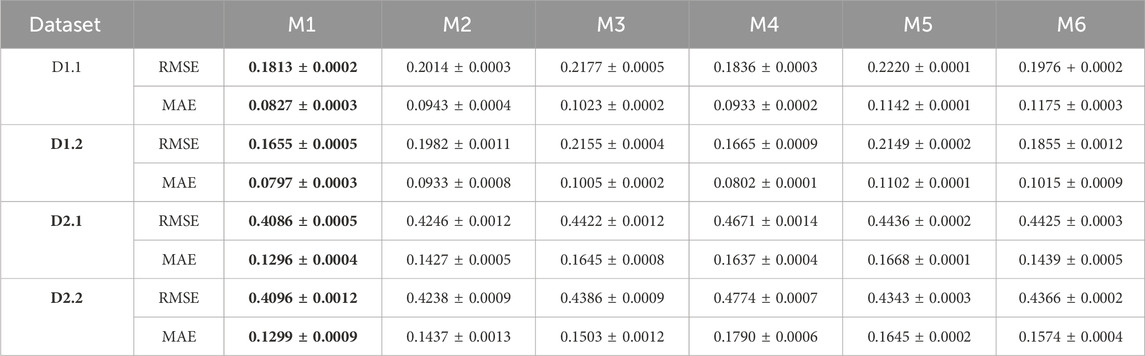
Table 5. Prediction error of all models.

Table 6

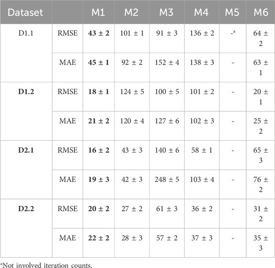
Table 6. Iteration count of all models.

Table 7

Table 7. Time cost of all models (seconds).

Figure 3

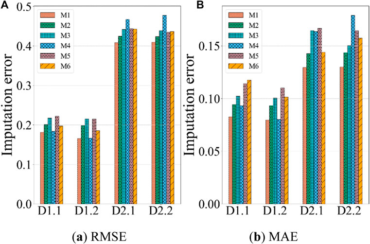
Figure 3. Performance comparison of M1-6 on four datasets. (A) RMSE, (B) MAE.

Figure 4

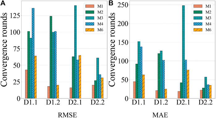
Figure 4. Iteration count comparison of M1-6 on four datasets. (A) RMSE, (B) MAE.

Figure 5

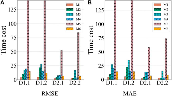
Figure 5. Time cost comparison of M1-6 on four datasets. (A) RMSE, (B) MAE.

6 Conclusion

In order to achieve the interpolation of PLM missing data, this paper proposes a LNTF model with low imputation error. In the LNTF model, we design two temporal-dependent linear biases to address the fluctuations of monitoring parameters. Further, we combine the advantages of L₁ and L₂ regularizations to accurately extract features of PLM data and improve the robustness of the LNTF model. In addition, the model parameters are updated by employing the NUM algorithm to accurately describe the nonnegativity of the PLM data. Finally, experiments on two datasets with different missing rates indicate that the LNTF model can effectively impute the PLM missing data, thereby providing a reliable data foundation for following data analysis. However, the following issues still need to be addressed:

• The manual tuning method for two hyper-parameters in LNTF consumes a lot of time. Therefore, it is a desirable work to incorporate the hyper-parameter adaptive learning scheme.

• Can we adopt other learning schemes such as ADMM algorithm (Hu et al., 2018; Luo et al., 2021d), second-order Newton’s method to update the model parameters?

We are aiming to address the above issues in future work.

Data availability statement

The original contributions presented in the study are included in the article/Supplementary Material, further inquiries can be directed to the corresponding author.

Author contributions

XL: Conceptualization, Funding acquisition, Investigation, Resources, Validation, Writing–original draft. ZH: Writing–review and editing, Conceptualization, Data curation, Supervision, Validation, Visualization. ZM: Project administration, Software, Writing–original draft. ZL: Formal Analysis, Validation, Writing–original draft. QW: Data curation, Methodology, Writing–original draft. AZ: Data curation, Validation, Writing–original draft.

Funding

The author(s) declare that financial support was received for the research, authorship, and/or publication of this article. This research was funded by Science and Technology Project of State Grid Jiangsu Electric Power Co., Ltd. (J2023017). The funder was not involved in the study design, collection, analysis, interpretation of data, the writing of this article, or the decision to submit it for publication.

Acknowledgments

Thanks for the funding provided by State Grid Jiangsu Electric Power Co., Ltd.

Conflict of interest

Authors XL, ZH, ZM, and ZL were employed by State Grid Jiangsu Electric Power Co., Ltd., Nanjing Power Supply Company.

The remaining authors declare that the research was conducted in the absence of any commercial or financial relationships that could be construed as a potential conflict of interest.

Publisher’s note

All claims expressed in this article are solely those of the authors and do not necessarily represent those of their affiliated organizations, or those of the publisher, the editors and the reviewers. Any product that may be evaluated in this article, or claim that may be made by its manufacturer, is not guaranteed or endorsed by the publisher.

References

Abubakar, I., Khalid, S. N., Mustafa, M. W., Shareef, H., and Mustapha, M. (2017). Application of load monitoring in appliances’ energy management–A review. Renew. Sustain. Energy Rev. 67, 235–245. doi:10.1016/j.rser.2016.09.064

CrossRef Full Text | Google Scholar

Alamoodi, A. H., Zaidan, B. B., Zaidan, A. A., Albahri, O., Chen, J., Chyad, M., et al. (2021). Machine learning-based imputation soft computing approach for large missing scale and non-reference data imputation. Chaos Solit. Fractals 151, 111236. doi:10.1016/j.chaos.2021.111236

CrossRef Full Text | Google Scholar

Allik, A., and Annuk, A. (2017). “Interpolation of intra-hourly electricity consumption and production data,” in Proceedings of the 6th international conference on renewable energy research and applications (San Diego, CA, USA), 131–136.

CrossRef Full Text | Google Scholar

Amritkar, R. E., and Kumar, P. P. (1995). Interpolation of missing data using nonlinear and chaotic system analysis. J. Geophys. Res. Atmos. 100, 3149–3154. doi:10.1029/94jd01531

CrossRef Full Text | Google Scholar

Badeau, R., Bertin, N., and Vincent, E. (2010). Stability analysis of multiplicative update algorithms and application to nonnegative matrix factorization. IEEE Trans. Neural Netw. 21, 1869–1881. doi:10.1109/tnn.2010.2076831

PubMed Abstract | CrossRef Full Text | Google Scholar

Batra, N., Gulati, M., and Singh, A. (2013). “It’s Different: insights into home energy consumption in India,” in Proceedings of the 5th ACM workshop on embedded systems for energy-efficient buildings (Roma, Italy), 1–8.

Google Scholar

Benjamin, B. M., and Yang, M. S. (2021). Weighted multiview possibilistic c-means clustering with L2 regularization. IEEE Trans. Fuzzy Syst. 30, 1357–1370. doi:10.1109/tfuzz.2021.3058572

CrossRef Full Text | Google Scholar

Bi, F., Luo, X., Shen, B., Dong, H., and Wang, Z. (2023). Proximal alternating-direction-method-of-multipliers-incorporated nonnegative latent factor analysis. IEEE/CAA J. Autom. Sin. 10, 1388–1406. doi:10.1109/jas.2023.123474

CrossRef Full Text | Google Scholar

Borges, C. E., Penya, Y. K., and Fernandez, I. (2012). Evaluating combined load forecasting in large power systems and smart grids. IEEE Trans. Ind. Inf. 9, 1570–1577. doi:10.1109/tii.2012.2219063

CrossRef Full Text | Google Scholar

Bulat, A., Kossaifi, J., and Tzimiropoulos, G. (2020). “Incremental multi-domain learning with network latent tensor factorization,” in Proceedings of the 34th AAAI conference on artificial intelligence (New York, NY, USA), 10470–10477.

CrossRef Full Text | Google Scholar

Chakhchoukh, Y., Panciatici, P., and Mili, L. (2010). Electric load forecasting based on statistical robust methods. IEEE Trans. Power Syst. 26, 982–991. doi:10.1109/tpwrs.2010.2080325

CrossRef Full Text | Google Scholar

Che, H., Pan, B., Leung, M. F., Cao, Y., and Yan, Z. (2023). Tensor factorization with sparse and graph regularization for fake news detection on social networks. IEEE Trans. Comput. Soc. Syst. 1, 1–11. doi:10.1109/tcss.2023.3296479

CrossRef Full Text | Google Scholar

Chen, J., Luo, X., and Zhou, M. C. (2021a). Hierarchical particle swarm optimization-incorporated latent factor analysis for large-scale incomplete matrices. IEEE Trans. Big Data 8, 1–1536. doi:10.1109/tbdata.2021.3090905

CrossRef Full Text | Google Scholar

Chen, K., Li, C., Li, A., Gao, J., and Ma, S. (2021b). “Focus on inherent attributes for temporal knowledge graph completion,” in Proceeding of the international joint conference on neural networks (Shenzhen, China), 1–8.

CrossRef Full Text | Google Scholar

Chen, M., Wang, R., Qiao, Y., and Luo, X. (2024). A generalized nesterov's accelerated gradient-incorporated non-negative latent-factorization-of-tensors model for efficient representation to dynamic QoS data. IEEE Trans. Emerg. Top. Comput. Intell. 1, 2386–2400. doi:10.1109/tetci.2024.3360338

CrossRef Full Text | Google Scholar

D’Incecco, M., Squartini, S., and Zhong, M. (2019). Transfer learning for non-intrusive load monitoring. IEEE Trans. Smart Grid 11, 1419–1429. doi:10.1109/tsg.2019.2938068

CrossRef Full Text | Google Scholar

Dong, J., Song, Y., Li, M., and Rao, H. (2024). Biased collective latent factorization of tensors with transfer learning for dynamic QoS data predicting. Digit. Signal Process. 146, 104360. doi:10.1016/j.dsp.2023.104360

CrossRef Full Text | Google Scholar

Duan, Y., Zhao, Y., and Hu, J. (2023). An initialization-free distributed algorithm for dynamic economic dispatch problems in microgrid: modeling, optimization and analysis. Sustain. Energy Grids Netw. 34, 101004. doi:10.1016/j.segan.2023.101004

CrossRef Full Text | Google Scholar

Gao, P., Wang, M., Chow, J. H., Berger, M., and Seversky, L. M. (2017). Missing data recovery for high-dimensional signals with nonlinear low-dimensional structures. IEEE Trans. Signal Process. 65 (20), 5421–5436. doi:10.1109/tsp.2017.2725227

CrossRef Full Text | Google Scholar

Grasmair, M., Scherzer, O., and Haltmeier, M. (2011). Necessary and sufficient conditions for linear convergence of ℓ1-regularization. Commun. Pure Appl. Math. 64, 161–182. doi:10.1002/cpa.20350

CrossRef Full Text | Google Scholar

Hafeez, G., Alimgeer, K. S., and Khan, I. (2020). Electric load forecasting based on deep learning and optimized by heuristic algorithm in smart grid. Appl. Energy 269, 114915. doi:10.1016/j.apenergy.2020.114915

CrossRef Full Text | Google Scholar

Hammad, M. A., Jereb, B., Rosi, B., and Dragan, D. (2020). Methods and models for electric load forecasting: a comprehensive review. Logist. Sustain. Transp. 11, 51–76. doi:10.2478/jlst-2020-0004

CrossRef Full Text | Google Scholar

He, J., Zhang, X., and Xu, B. (2019). KF-based multiscale response reconstruction under unknown inputs with data fusion of multitype observations. J. Aerosp. Eng. 32 (4), 04019038. doi:10.1061/(asce)as.1943-5525.0001031

CrossRef Full Text | Google Scholar

Hu, L., Yang, S., and Luo, X. (2020). An algorithm of inductively identifying clusters from attributed graphs. IEEE Trans. Big Data 8, 523–534. doi:10.1109/TBDATA.2020.2964544

CrossRef Full Text | Google Scholar

Hu, L., Yang, S., Luo, X., Yuan, H., Sedraoui, K., and Zhou, M. (2021). A distributed framework for large-scale protein-protein interaction data analysis and prediction using mapreduce. IEEE/CAA J. Autom. Sin. 9, 160–172. doi:10.1109/jas.2021.1004198

CrossRef Full Text | Google Scholar

Hu, L., Yuan, X., Liu, X., Xiong, S., and Luo, X. (2018). Efficiently detecting protein complexes from protein interaction networks via alternating direction method of multipliers. IEEE/ACM Trans. Comput. Biol. Bioinform. 16, 1922–1935. doi:10.1109/tcbb.2018.2844256

PubMed Abstract | CrossRef Full Text | Google Scholar

Jin, Y. F., Yin, Z. Y., Zhou, W. H., Yin, J. H., and Shao, J. F. (2019). A single-objective EPR based model for creep index of soft clays considering L2 regularization. Eng. Geol. 248, 242–255. doi:10.1016/j.enggeo.2018.12.006

CrossRef Full Text | Google Scholar

Kelly, J., and Knottenbelt, W. (2015). The UK-DALE dataset, domestic appliance-level electricity demand and whole-house demand from five UK homes. Sci. Data 2, 150007–150014. doi:10.1038/sdata.2015.7

PubMed Abstract | CrossRef Full Text | Google Scholar

Kilmer, M. E., and Martin, C. D. (2011). Factorization strategies for third-order tensors. Linear Algebra Appl. 435 (3), 641–658. doi:10.1016/j.laa.2010.09.020

CrossRef Full Text | Google Scholar

Li, H., Zhang, Q., and Deng, J. (2016). Biased multiobjective optimization and decomposition algorithm. IEEE Trans. Cybern. 47, 52–66. doi:10.1109/tcyb.2015.2507366

PubMed Abstract | CrossRef Full Text | Google Scholar

Li, P., Hu, J., Qiu, L., Zhao, Y., and Ghosh, B. K. (2021). A distributed economic dispatch strategy for power–water networks. IEEE Trans. Control Netw. Syst. 9, 356–366. doi:10.1109/tcns.2021.3104103

CrossRef Full Text | Google Scholar

Li, W., Luo, X., Yuan, H., and Zhou, M. (2022b). A momentum-accelerated Hessian-vector-based latent factor analysis model. IEEE Trans. Serv. Comput. 16, 830–844. doi:10.1109/tsc.2022.3177316

CrossRef Full Text | Google Scholar

Li, Z., Li, S., Bamasag, O. O., Alhothali, A., and Luo, X. (2022a). Diversified regularization enhanced training for effective manipulator calibration. IEEE Trans. Neural Netw. Learn. Syst. 34, 8778–8790. doi:10.1109/tnnls.2022.3153039

CrossRef Full Text | Google Scholar

Liu, J., Musialski, P., Wonka, P., and Ye, J. (2012). Tensor completion for estimating missing values in visual data. IEEE Trans. Pattern Anal. Mach. Intell. 35 (1), 208–220. doi:10.1109/tpami.2012.39

PubMed Abstract | CrossRef Full Text | Google Scholar

Liu, Z., Luo, X., and Wang, Z. (2020). Convergence analysis of single latent factor-dependent, nonnegative, and multiplicative update-based nonnegative latent factor models. IEEE Trans. Neural Netw. Learn. Syst. 32, 1737–1749. doi:10.1109/tnnls.2020.2990990

CrossRef Full Text | Google Scholar

Liu, Z., Luo, X., and Zhou, M. (2023). Symmetry and graph bi-regularized non-negative matrix factorization for precise community detection. IEEE Trans. Autom. Sci. Eng. 21, 1406–1420. doi:10.1109/tase.2023.3240335

CrossRef Full Text | Google Scholar

Luo, L., Li, Y. F., and Haffari, G. (2023). “Normalizing flow-based neural process for few-shot knowledge graph completion,” in Proceedings of the 46th international ACM SIGIR conference on research and development in information retrieval (Taiwan, China), 900–910.

CrossRef Full Text | Google Scholar

Luo, X., Chen, M., Wu, H., Liu, Z., Yuan, H., and Zhou, M. (2021a). Adjusting learning depth in nonnegative latent factorization of tensors for accurately modeling temporal patterns in dynamic QoS data. IEEE Trans. Autom. Sci. Eng. 18, 2142–2155. doi:10.1109/tase.2020.3040400

CrossRef Full Text | Google Scholar

Luo, X., Wang, Z., and Shang, M. (2019c). An instance-frequency-weighted regularization scheme for non-negative latent factor analysis on high-dimensional and sparse data. IEEE Trans. Syst. Man. Cybern. Syst. 51, 3522–3532. doi:10.1109/tsmc.2019.2930525

CrossRef Full Text | Google Scholar

Luo, X., Wu, H., and Li, Z. (2022). NeuLFT: a novel approach to nonlinear canonical polyadic decomposition on high-dimensional incomplete tensors. IEEE Trans. Knowl. Data Eng. 35, 1–6166. doi:10.1109/tkde.2022.3176466

CrossRef Full Text | Google Scholar

Luo, X., Wu, H., Wang, Z., Wang, J., and Meng, D. (2021c). A novel approach to large-scale dynamically weighted directed network representation. IEEE Trans. Pattern Anal. Mach. Intell. 44, 9756–9773. doi:10.1109/tpami.2021.3132503

CrossRef Full Text | Google Scholar

Luo, X., Wu, H., Yuan, H., and Zhou, M. (2019a). Temporal pattern-aware QoS prediction via biased non-negative latent factorization of tensors. IEEE Trans. Cybern. 50, 1798–1809. doi:10.1109/tcyb.2019.2903736

PubMed Abstract | CrossRef Full Text | Google Scholar

Luo, X., Zhong, Y., Wang, Z., and Li, M. (2021d). An alternating-direction-method of multipliers-incorporated approach to symmetric non-negative latent factor analysis. IEEE Trans. Neural Netw. Learn. Syst. 34, 4826–4840. doi:10.1109/tnnls.2021.3125774

CrossRef Full Text | Google Scholar

Luo, X., Zhou, M. C., Li, S., Hu, L., and Shang, M. (2019b). Non-negativity constrained missing data estimation for high-dimensional and sparse matrices from industrial applications. IEEE Trans. Cybern. 50, 1844–1855. doi:10.1109/tcyb.2019.2894283

PubMed Abstract | CrossRef Full Text | Google Scholar

Luo, X., Zhou, M. C., Li, S., Xia, Y., You, Z. H., Zhu, Q., et al. (2017). Incorporation of efficient second-order solvers into latent factor models for accurate prediction of missing QoS data. IEEE Trans. Cybern. 48, 1216–1228. doi:10.1109/tcyb.2017.2685521

PubMed Abstract | CrossRef Full Text | Google Scholar

Luo, X., Zhou, M. C., Li, S., You, Z., Xia, Y., and Zhu, Q. (2015). A nonnegative latent factor model for large-scale sparse matrices in recommender systems via alternating direction method. IEEE Trans. Neural Netw. Learn. Syst. 27, 579–592. doi:10.1109/tnnls.2015.2415257

PubMed Abstract | CrossRef Full Text | Google Scholar

Luo, X., Zhou, Y., Liu, Z., and Zhou, M. (2021b). Fast and accurate non-negative latent factor analysis of high-dimensional and sparse matrices in recommender systems. IEEE Trans. Knowl. Data Eng. 35, 3897–3911. doi:10.1109/tkde.2021.3125252

CrossRef Full Text | Google Scholar

Miao, X., Gao, Y., Chen, G., Zheng, B., and Cui, H. (2016). Processing incomplete k nearest neighbor search. IEEE Trans. Fuzzy Syst. 24 (6), 1349–1363. doi:10.1109/tfuzz.2016.2516562

CrossRef Full Text | Google Scholar

Nie, Y., Jia, Y., Li, S., Zhu, X., and Zhou, B. (2016). Identifying users across social networks based on dynamic core interests. Neurocomputing 210, 107–115. doi:10.1016/j.neucom.2015.10.147

CrossRef Full Text | Google Scholar

Qin, W., and Luo, X. (2023). Asynchronous parallel fuzzy stochastic gradient descent for high-dimensional incomplete data representation. IEEE Trans. Fuzzy Syst. 32, 445–459. doi:10.1109/tfuzz.2023.3300370

CrossRef Full Text | Google Scholar

Qin, W., Luo, X., and Zhou, M. C. (2023). Adaptively-accelerated parallel stochastic gradient descent for high-dimensional and incomplete data representation learning. IEEE Trans. Big Data 10, 92–107. doi:10.1109/tbdata.2023.3326304

CrossRef Full Text | Google Scholar

Qin, W., Wang, H., Zhang, F., Wang, J., Luo, X., and Huang, T. (2022). Low-rank high-order tensor completion with applications in visual data. IEEE Trans. Image Process. 31, 2433–2448. doi:10.1109/tip.2022.3155949

PubMed Abstract | CrossRef Full Text | Google Scholar

Shang, M., Yuan, Y., Luo, X., and Zhou, M. (2021). An α–β-divergence-generalized recommender for highly accurate predictions of missing user preferences. IEEE Trans. Cybern. 52, 8006–8018. doi:10.1109/tcyb.2020.3026425

CrossRef Full Text | Google Scholar

Shao, B., Xiao, Q., Xiong, L., Wang, L., Yang, Y., Chen, Z., et al. (2023). Power coupling analysis and improved decoupling control for the VSC connected to a weak AC grid. Int. J. Electr. Power Energy Syst. 145, 108645. doi:10.1016/j.ijepes.2022.108645

CrossRef Full Text | Google Scholar

Shirkhani, M., Tavoosi, J., Danyali, S., Sarvenoee, A. K., Abdali, A., Mohammadzadeh, A., et al. (2023). A review on microgrid decentralized energy/voltage control structures and methods. Energy Rep. 10, 368–380. doi:10.1016/j.egyr.2023.06.022

CrossRef Full Text | Google Scholar

Song, J., Mingotti, A., Zhang, J., Peretto, L., and Wen, H. (2022). Accurate damping factor and frequency estimation for damped real-valued sinusoidal signals. IEEE Trans. Instrum. Meas. 71, 1–4. doi:10.1109/tim.2022.3220300

CrossRef Full Text | Google Scholar

Su, X., Zhang, M., Liang, Y., Cai, Z., Guo, L., and Ding, Z. (2021). A tensor-based approach for the QoS evaluation in service-oriented environments. IEEE Trans. Netw. Serv. Manag. 18, 3843–3857. doi:10.1109/tnsm.2021.3074547

CrossRef Full Text | Google Scholar

Tabatabaei, S. M., Dick, S., and Xu, W. (2016). Toward non-intrusive load monitoring via multi-label classification. IEEE Trans. Smart Grid 8, 26–40. doi:10.1109/tsg.2016.2584581

CrossRef Full Text | Google Scholar

Wang, H., Xu, Z., Ge, X., Liao, Y., Yang, Y., Zhang, Y., et al. (2023). A junction temperature monitoring method for IGBT modules based on turn-off voltage with convolutional neural networks. IEEE Trans. Power Electron. 38, 10313–10328. doi:10.1109/tpel.2023.3278675

CrossRef Full Text | Google Scholar

Wang, L., Zhang, Y., and Feng, J. (2005). On the Euclidean distance of images. IEEE Trans. Pattern Anal. Mach. Intell. 27, 1334–1339. doi:10.1109/tpami.2005.165

PubMed Abstract | CrossRef Full Text | Google Scholar

Wang, M. C., Tsai, C. ; F., and Lin, W. C. (2021). Towards missing electric power data imputation for energy management systems. Expert Syst. Appl. 174, 114743. doi:10.1016/j.eswa.2021.114743

CrossRef Full Text | Google Scholar

Wang, Q., Chen, M., Shang, M., and Luo, X. (2019). A momentum-incorporated latent factorization of tensors model for temporal-aware QoS missing data prediction. Neurocomputing 367, 299–307. doi:10.1016/j.neucom.2019.08.026

CrossRef Full Text | Google Scholar

Wang, S., Ma, Y., Cheng, B., Yang, F., and Chang, R. N. (2016). Multi-dimensional QoS prediction for service recommendations. IEEE Trans. Serv. Comput. 12, 47–57. doi:10.1109/tsc.2016.2584058

CrossRef Full Text | Google Scholar

Wang, S., Zheng, C., Ma, T., Wang, T., Gao, S., Dai, Q., et al. (2024). Tooth backlash inspired comb-shaped single-electrode triboelectric nanogenerator for self-powered condition monitoring of gear transmission. Nano Energy 123, 109429. doi:10.1016/j.nanoen.2024.109429

CrossRef Full Text | Google Scholar

Wu, D., He, Y., and Luo, X. (2023c). A graph-incorporated latent factor analysis model for high-dimensional and sparse data. IEEE Trans. Emerg. Top. Comput. 11, 907–917. doi:10.1109/tetc.2023.3292866

CrossRef Full Text | Google Scholar

Wu, D., Li, Z., Yu, Z., He, Y., and Luo, X. (2023a). Robust low-rank latent feature analysis for spatiotemporal signal recovery. IEEE Trans. Neural Netw. Learn. Syst. 1, 1–14. doi:10.1109/tnnls.2023.3339786

CrossRef Full Text | Google Scholar

Wu, D., Luo, X., He, Y., and Zhou, M. (2022a). A prediction-sampling-based multilayer-structured latent factor model for accurate representation to high-dimensional and sparse data. IEEE Trans. Neural Netw. Learn. Syst. 35, 3845–3858. doi:10.1109/tnnls.2022.3200009

CrossRef Full Text | Google Scholar

Wu, D., Luo, X., Shang, M., He, Y., Wang, G., and Zhou, M. (2019). A deep latent factor model for high-dimensional and sparse matrices in recommender systems. IEEE Trans. Syst. Man. Cybern. Syst. 51, 4285–4296. doi:10.1109/tsmc.2019.2931393

CrossRef Full Text | Google Scholar

Wu, D., Shang, M., Luo, X., and Wang, Z. (2021c). An L 1-and-L 2-norm-oriented latent factor model for recommender systems. IEEE Trans. Neural Netw. Learn. Syst. 33, 5775–5788. doi:10.1109/tnnls.2021.3071392

CrossRef Full Text | Google Scholar

Wu, D., Zhang, P., He, Y., and Luo, X. (2022b). A double-space and double-norm ensembled latent factor model for highly accurate web service QoS prediction. IEEE Trans. Serv. Comput. 16, 802–814. doi:10.1109/tsc.2022.3178543

CrossRef Full Text | Google Scholar

Wu, D., Zhang, P., He, Y., and Luo, X. (2023b). MMLF: multi-metric latent feature analysis for high-dimensional and incomplete data. IEEE Trans. Serv. Comput. 17, 575–588. doi:10.1109/tsc.2023.3331570

CrossRef Full Text | Google Scholar

Wu, H., and Luo, X. (2021). “Instance-frequency-weighted regularized, nonnegative and adaptive latent factorization of tensors for dynamic QoS analysis,” in Proceedings of the 28th international conference on web services (Chicago, IL, USA: Virtual Event), 560–568.

CrossRef Full Text | Google Scholar

Wu, H., Luo, X., and Zhou, M. C. (2020). Advancing non-negative latent factorization of tensors with diversified regularization schemes. IEEE Trans. Serv. Comput. 15, 1334–1344. doi:10.1109/tsc.2020.2988760

CrossRef Full Text | Google Scholar

Wu, H., Luo, X., and Zhou, M. C. (2021b). “Neural latent factorization of tensors for dynamically weighted directed networks analysis,” in Proceedings of the international conference on systems, man, and cybernetics 2021 (Melbourne, Australia), 3061–3066.

CrossRef Full Text | Google Scholar

Wu, H., Luo, X., Zhou, M. C., Rawa, M. J., Sedraoui, K., and Albeshri, A. (2021a). A PID-incorporated latent factorization of tensors approach to dynamically weighted directed network analysis. IEEE/CAA J. Autom. Sin. 9, 533–546. doi:10.1109/jas.2021.1004308

CrossRef Full Text | Google Scholar

Xu, X., Lin, M., Luo, X., and Xu, Z. (2023). HRST-LR: a hessian regularization spatio-temporal low rank algorithm for traffic data imputation. IEEE Trans. Intell. Transp. Syst. 24, 11001–11017. doi:10.1109/tits.2023.3279321

CrossRef Full Text | Google Scholar

Yang, T., Xu, J., and Fei, L. I. (2023b). Electric theft detection based on optimal transform correlation factor and optimized shift-splitting iteration method. Power Syst. Technol. 47, 3913–3924. doi:10.2139/ssrn.4353843

CrossRef Full Text | Google Scholar

Yang, Y., and Nagarajaiah, S. (2016). Harnessing data structure for recovery of randomly missing structural vibration responses time history: sparse representation versus low-rank structure. Mech. Syst. Signal Process. 74, 165–182. doi:10.1016/j.ymssp.2015.11.009

CrossRef Full Text | Google Scholar

Yang, Y., Wei, X., Yao, W., and Lan, J. (2023a). Broadband electrical impedance matching of sandwiched piezoelectric ultrasonic transducers for structural health monitoring of the rail in-service. Sens. Actuators A Phys. 364, 114819. doi:10.1016/j.sna.2023.114819

CrossRef Full Text | Google Scholar

Ye, F., Lin, Z., and Chen, C. (2021). “Outlier-resilient web service qos prediction,” in Proceedings of the web conference 2021 (Ljubljana, Slovenia), 3099–3110.

CrossRef Full Text | Google Scholar

Yuan, Y., Luo, X., Shang, M., and Wang, Z. (2022). A Kalman-filter-incorporated latent factor analysis model for temporally dynamic sparse data. IIEEE Trans. Cybern. 53, 5788–5801. doi:10.1109/tcyb.2022.3185117

CrossRef Full Text | Google Scholar

Yuan, Y., Luo, X., and Shang, M. S. (2018). Effects of preprocessing and training biases in latent factor models for recommender systems. Neurocomputing 275, 2019–2030. doi:10.1016/j.neucom.2017.10.040

CrossRef Full Text | Google Scholar

Zeng, S., Gou, J., and Deng, L. (2017). An antinoise sparse representation method for robust face recognition via joint l1 and l2 regularization. Expert Syst. Appl. 82, 1–9. doi:10.1016/j.eswa.2017.04.001

CrossRef Full Text | Google Scholar

Zhang, H., Wu, H., Jin, H., and Li, H. (2022). High-dynamic and low-cost sensorless control method of high-speed brushless DC motor. IEEE Trans. Ind. Inf. 19, 5576–5584. doi:10.1109/tii.2022.3196358

CrossRef Full Text | Google Scholar

Zhang, X., Gong, L., Zhao, X., Li, R., Yang, L., and Wang, B. (2023). Voltage and frequency stabilization control strategy of virtual synchronous generator based on small signal model. Energy Rep. 9, 583–590. doi:10.1016/j.egyr.2023.03.071

CrossRef Full Text | Google Scholar

Zhang, Z., Zhuang, F., and Zhu, H. (2020). “Relational graph neural network with hierarchical attention for knowledge graph completion,” in Proceedings of the 34th AAAI conference on artificial intelligence (New York, NY, USA), 9612–9619.

CrossRef Full Text | Google Scholar

Zhao, M., Wu, L., and Liang, Y. (2022). “Investigating accuracy-novelty performance for graph-based collaborative filtering,” in Proceedings of the 45th international ACM SIGIR conference on research and development in information retrieval (Madrid, Spain), 50–59.

CrossRef Full Text | Google Scholar

Zhao, X., Jia, Y., Li, A., Jiang, R., Chen, K., and Wang, Y. (2021). Target relational attention-oriented knowledge graph reasoning. Neurocomputing 461, 577–586. doi:10.1016/j.neucom.2021.03.135

CrossRef Full Text | Google Scholar