 Shiyao Hu
 Chunyan Rong1
- 1Economic and Technology Research Institute of State Grid Hebei Electric Power Co., Ltd., Shijiazhuang, Hebei, China
- 2School of Electrical and Control Engineering, North China University of Technology, Beijing, China
With the connection and integration of renewable energy, the on-load tap-changer (OLTC) has become an important device for regulating voltage in distribution networks. However, due to non-smooth and non-linear characteristics of OLTC, traditional bad data identification and state estimation methods for transmission network are limited when applied to the distribution network. Therefore, the nonlinearity and droop control constraints of the OLTC model are considered in this paper. At the same time, the quadratic penalty function is introduced to realize the fast normalization of the tap position. It proposes a two-stage bad data identification method based on mixed-integer linear programming. In the first stage, suspicious measurements are identified using projection statistics and maximum normalized residual methods for preprocessing the measurement data. In the second stage, a linearization approach utilizing hyhrid data-physical driven is applied to handle nonlinear constraints, leading to the development of a bad data identification model based on mixed-integer linear programming. Finally, the proposed methodology is validated using a modified IEEE-33 node test feeder example, demonstrating the accuracy and efficiency of bad data identification.
1 Introduction
In the context of distribution network state estimation, the integrity of the estimation process can be compromised by the presence of erroneous data. Such data may arise from a variety of sources, including heterogeneous measurement instruments, sensor failures, and communication disruptions. These inaccuracies have the potential to severely impact the reliability and accuracy of the state estimation outcomes (Chen et al., 2021). The same time, With the continuous integration of renewable energy sources, OLTC is increasingly being utilized in power grid applications every year. It plays an important role in ensuring the safe and reliable operation of distribution networks and grid dispatching (Ju and Huang, 2023).The relevant parameters of the on-load tap-changer device exhibit nonlinearity and discreteness in mathematical models, and traditional continuous variable processing methods may reduce the accuracy of state estimation.
Traditional methods for bad data identification primarily encompass residual search methods (Handschin et al., 1975; Lin and Abur, 2018; Zhao and Mill, 2018), zero residual methods (Zhuang and Balasubramanian, 1987), and estimation-based methods (Huang and Lin, 2004). These approaches are susceptible to errors such as misjudgment and missed detection. Contemporary techniques for bad data detection and identification predominantly include optimization-based and intelligent algorithm-based approaches. Among these, optimization-based methods have demonstrated a significant capacity for accurate identification of erroneous measurement data. A literature (Irving, 2008) proposes a robust state estimation model based on mixed integer nonlinear programming (MINLP). This method has high accuracy in identifying bad data, but lacks precision in estimation. Additionally, the model is nonconvex, nonlinear, and introduces a large number of 0/1 integer variables, making it difficult to solve. When the scale of the system increases, the solution efficiency de-creases. The Schweppe-type generalized M-estimator with Huber psi-function (SHGM) is currently a method with good robustness (Mili et al., 1996). Introduces coefficients that reflect the lever-age properties, which can suppress the weight of bad data in leverage points and weaken the effect of bad data residuals in the objective function. However, it cannot completely filter out the impact of bad data. Existing methods need further improvement in terms of computational efficiency, accuracy, and ability to handle bad data.
For state estimation problems involving discrete variables, modelling and solving based on MINLP methods may have low convergence and computational efficiency. In order to avoid solving MINLP problems, in traditional state estimation, OLTC tap positions are usually treated as continuous variables (Shiroi and Hosseinie, 2008), which may lead to biases in the estimated results due to mismatch with the actual operating characteristics of OLTC. The literature (Korres et al., 2004; Teixeira et al., 1992; Handschin and Kliokys, 1995) presents, in addition to the traditional treatment of continuous variables, using rounding or sensitivity analysis to round the tap positions to integers. These integer values are then taken as known parameters and used in the state estimation problem to solve state variables such as voltage magnitude and phase angle. The literature (Maalouf et al., 2013) develops a mixed integer quadratic programming model with discrete variables, which can effectively address the tap position rounding issue with high accuracy, although the approach is more complex. Furthermore, the literature (Nanchian et al., 2017) applies a hybrid particle swarm optimization method to solve MINLP problems that involve discrete tap positions, but the algorithm has a long computation time and low efficiency.
To address the challenges of nonlinearity and low efficiency in bad data identification for OLTC discrete variables, this paper introduces a two-stage bad data identification method utilizing a positive curvature quadratic penalty function to facilitate rapid adjustment of OLTC tap positions. This method enhances solution efficiency while maintaining the accuracy of identification. The main contributions are as follows:
1) In order to improve the accuracy of bad data identification, an optimization-based method for bad data identification is proposed in this paper. This method can accurately and effectively identify the presence of bad data in the measurement data, demonstrating a good identification accuracy.
2) To cope with the issue of low efficiency in solving traditional MINLP models due to a large number of discrete and nonlinear constraints, this paper presents a two-stage bad data identification model based on mixed integer linear programming (MILP). In the first stage, all measurements are distinguished using projection statistics and maximum normalized residual methods, generating a reduced set of suspicious measurements. In the second stage, a linearization model based on hyhrid data-physical driven is proposed to linearize nonlinear constraints, leading to a MILP-based bad data identification method that significantly improves the accuracy and efficiency of bad data identification.
The organizational structure of this paper is as follows: Section 2 introduces the method of identifying leverage points and suspicious measurement bad data based on projection statistics and maximum normalized residual method, and obtains the reduction of suspicious measurement set; Section 3 introduces the traditional MINLP bad data identification model, and proposes a hyhrid data-physical driven linearization model considering OLTC constraints, and constructs a bad data identification model based on MILP; Section 4 illustrates the experimental at IEEE-33 node test feeder; Section 5 provides the conclusion.
2 Stage 1: reduction of suspicious measurement set
In this paper, the reduced suspicious measurement set mainly consists of two parts. The first part involves the identification of leverage points through the use of projection statistics, while the second part involves the identification of suspicious measurements in non-leverage points using the maximum normalized residual method. The detailed explanation of the two algorithm processes is provided below.
2.1 Identification of leveraged measurements using projection statistics
This subsection describes the mathematical model for identifying leverage points based on projection statistics. Firstly, the connotation of leverage points and their impact on state estimation are introduced. Currently, there are two types of definitions for leverage points. As shown in Figure 1, the first type is based on regression model analysis, while the second type is based on the analysis of diagonal elements of the hat matrix. The difference between the two methods is as follows: The first type constructs a factor space composed of the measurement Jacobian matrix and the measurement vector, obtaining the distribution of row vectors in each group of measurement Jacobian matrix and the measurement vector in the factor space, and identifies outliers as leverage points; the second type is based on residual sensitivity analysis, namely, determining whether the measurement residual increases significantly when there is a large measurement error in the system, and identifying measurements where the measurement error cannot be positively fed back to the measurement residual as leverage points.
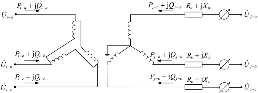
Figure 1. Dy11 on-load tap changer equivalent model.
The first method based on regression model analysis is introduced as follows. The first-order Taylor expansion is performed at the initial value point
Where,
The above Equation 1 is called the regression analysis model in statistics.
Due to the system network parameters, measurement errors, and other reasons, abnormal values may appear in the above factor space, that is, the data is quite different from other data, and it is shown as outliers in the two-dimensional space. When outliers appear in the Y-space ' of the factor space, that is, in the ordinate axis '
To identify outliers in the “X-space,” that is, to identify anomalies in the row vectors of the Jacobian matrix compared to other row vectors, this can be achieved by calculating distance measures between the individual row vectors. The Mahalanobis distance and other similar distance measures based on this can be used to calculate the distances between the row vectors. The criterion of such methods is to compare the distance between the row vectors with a set threshold. Measurements greater than this threshold are considered leverage measurements. The threshold setting criterion is to designate measurements that are far from most other measurements as leverage measurements. However, in cases where there are multiple leverage measurements in a system, problems may arise due to mutual masking between the leverage measurements, causing this type of method to potentially struggle to accurately identify systems with multiple leverage measurements.
The second method based on residual sensitivity analysis is introduced as follows. The estimation of the measurement error based on the least square method is defined as
Where,
When Equations 1, 2, the measurement residual is defined as the difference between the measured value and the estimated measurement vector, which can be equivalent to the error between the estimated measurement error value
In the equation,
The hat matrix
From the above equation, Based on Equation 3, we know that when the diagonal elements of are close to 0. If the measurement error is large and the diagonal elements of the multiplication of the sensitivity matrix remains very small, indicating that the measurement error cannot be reflected in the residual of the measurement, then define this type of measurement as a leverage measurement. Furthermore, the leverage measurement can also be determined by comparing with its expected value to assess its relative magnitude.
The expected value is calculated as shown in Equation 6:
If
To avoid the difficult identification of leverage measurements that may arise from the two aforementioned methods, this paper adopts a method based on projection statistical values for the identification of leverage measurement. This method circumvents the calculation problem of the covariance matrix and directly utilizes the projections of the row vectors of the Jacobian matrix onto the relevant subspace to identify leverage measurements. First, calculate the projection statistical values for all measurements, with the calculation formula as follows:
Where
The calculation formula for
Where,
After calculating the projection statistical values corresponding to each measurement based on Equations 7, 8, compare them numerically with the projection statistical cutoff values. Under a Gaussian distribution, the projection statistics typically follow a Chi-square distribution, satisfying Equation 9:
Where,
When comparing the calculated projection statistical values with the cut off values, you can determine whether the measurement is a leverage measurement based on the comparison results.
If the calculated projection statistical value D for measurement
2.2 Identification of suspicious bad data using maximum normalized residual method
As the calculation of residuals is approximate to the error values, it may not be able to detect bad data. By using standardized residuals, a more accurate method for identifying bad data can be obtained. The normalized residual value for measurement i can be obtained by dividing the residual value by the corresponding diagonal element in the residual covariance matrix.
In Equation 11:
In Equation 12:
When solving the weighted least squares state estimation, the residual value can be calculated. The calculation formula is as shown in Equation 13:
For non-leverage measurement, the normalized residual vector
Therefore, the maximum element in
3 Stage 2: bad data identification based on mixed integer linear programming
In order to improve the solving efficiency of the traditional MINLP model, the hybrid data-physical-driven linearization model is first applied to linearize the non-linear constraints in the state estimation of on-load tap changer in transformers. Subsequently, an MILP-based bad data identification model is constructed. The following provides a detailed description of the linearization process and the construction of the optimization model.
3.1 Bad data identification based on MINLP
The traditional MINLP-based bad data identification model is represented as follows:
In Equations 15–18:
The bad data identification method based on mixed integer can overcome the problem that the residual method is difficult to identify the bad data of the multi-leverage measurement system, and has high identification accuracy. However, due to the serious non-convex nonlinearity of the model, the requirement for the solver is high, and the computational efficiency of the model solution is low.
3.2 The hybrid data-physical-driven measurement equation linearization model
3.2.1 OLTC model considering non-smooth control characteristics
OLTC includes two parts, “transformer” and “tap changer.” Unlike traditional transformers, an OLTC sets the tap position as an unknown variable during modelling. By controlling the amplitude of the secondary side voltage to meet a certain dead band range, the OLTC adjusts the tap position to maintain the voltage level at the load center within a certain error range, thereby enhancing the power quality for the user. This paper proposes a droop control model for the OLTC, where the amplitude of the secondary side voltage and the tap turns ratio of the OLTC align with the droop control curve.
Define the column name of the nodal association matrix to represent the node
Where represents the association between a branch and a node, with its direction flowing out of the node; and represents the association between a branch and a node, with its direction flowing into the node.
Taking phase A as an example, according to the law of energy conservation on the primary and secondary sides of the transformer, the voltage and current on the winding satisfy the following relationship:
Here,
The relationship between branch current and node voltage is expressed as shown in Equation 21:
Equation 20 is expressed as a matrix as shown in Equation 22:
Similarly, the relationship between the branch current and node voltage for phases B and C is derived, and the relationship between the three-phase branch current and voltage is ultimately obtained as follows:
In Equation 23:
By combining the original admittance matrix with the node-branch incidence matrix, the node admittance matrix is obtained from the following equation:
The branch power connected to each node is calculated using the node injection power expression as shown in Equations 24 and 25:
The following describes the modelling of the regulator part in Figure 2.
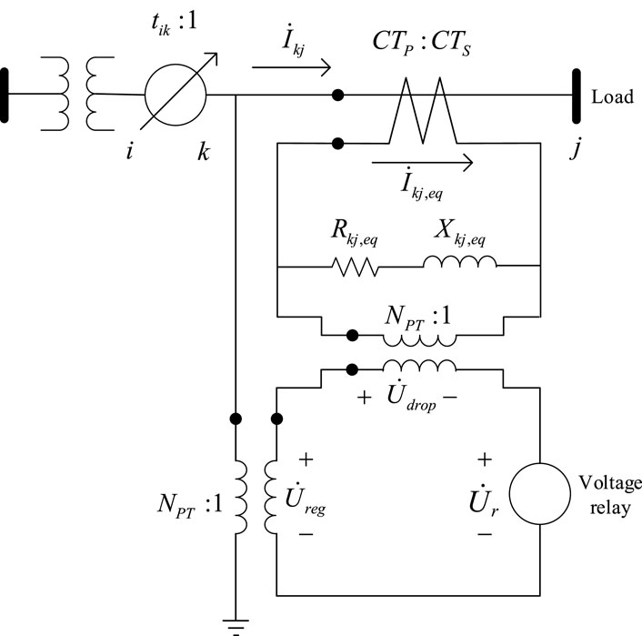
Figure 2. Detailed schematic diagram of OLTC voltage regulator part.
The tap position of OLTC are regulated through a control circuit. When voltage control, direct control cannot be carried out on the high-voltage circuit. Therefore, voltage and current transformers are used to construct a simulated circuit - the control circuit. The control circuit is a proportional model of the actual line. For example, if the actual line transformer has a secondary side rated at 2.4 kV, the control circuit operates at a voltage level of 120 V. By monitoring the voltage of the control circuit, the voltage at the load center of the actual line can be determined. If the voltage is below the normal level, indicating that the voltage at the loading center is below the position of the normal level, the tap changer is adjusted to raise the voltage at the loading center. For three-phase supply voltages below 10 kV, the allowable deviation is 7% of the rated voltage. For single-phase supply voltages of 220 V, the allowable deviation is +7% and −10% of the rated voltage.
For the control circuit, the current rating of the primary winding of the current transformer is set as
It should be noted that the equivalent impedance of the three-phase line is not the actual line impedance; it is the turns ratio of the actual measured voltage on the secondary side to the load center voltage difference to the load side current under the rated turns ratio.
The equivalent impedance of the line compensator is calculated from the equivalent impedance of the three-phase line as
The current in the compensator branch is obtained from the actual line current
In Equation 28:
The voltage difference
Finally, the control voltage of the compensator branch is as shown in Equation 30:
Applying the droop control to the control voltage and tap changer turns ratio, taking phase A as an example, the principle of droop control for the OLTC is introduced. Define
The physical meaning of the above equation is that when the control voltage is within the dead zone, the OLTC tap position remains unchanged.
The
The relationship between
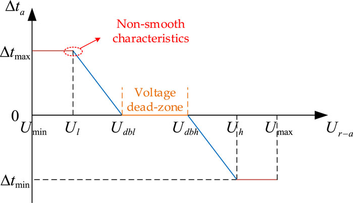
Figure 3. Voltage regulation control curve showing the variation of the turns ratio with control voltage droop.
Where,
The relationship between the droop control coefficient and the variation in the turns ratio and the voltage is as shown in Equation 33:
From Figure 3, it can be seen that the characteristic curve represents a piecewise function. When the system operates near the turning point, the derivative is discontinuous, the algorithm search direction is uncertain, and it is difficult to smoothly switch operating curves, so the piecewise droop control function has strong non-smooth characteristics and is difficult to solve. Usually, mixed integer nonlinear programming is used to describe piecewise function control characteristics, but this method has low computational efficiency. In this paper, a fitting function is used to approximate the piecewise function, and the fitted droop control function is shown in Equation 34:
Where,
Approximately fitting the piecewise droop control function can transform it into a smooth function that is continuously differentiable, as shown in Figure 4. The smoothing function can avoid sudden changes in derivative order during algorithm iteration calculations, thus improving the convergence of the algorithm.
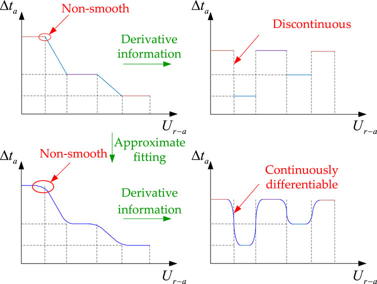
Figure 4. Derivative comparison diagram before and after fitting.
The variation of the ratio of the voltage regulator and the tap variable satisfies the relationship is shown in Equation 34:
In the equation,
In this paper, the discrete tap-changer variable is first treated as a continuous variable for state estimation calculations to obtain a continuous optimal solution for state estimation. Subsequently, a positive curvature quadratic penalty function is introduced in the objective function, and the state estimation is continued using the continuous optimal solution as the initial value to obtain an integer solution for the tap-changer setting.
Taking phase A as an example, the positive curvature quadratic penalty function is shown in Figure 5.
Figure 5. Quadratic penalty function model.
Where,
In the optimization process, when the value of
In the equation,
From Equation 38, it can be observed that for the Newton method, the introduction of a penalty function in the objective function will result in the incremental inclusion of the first and second derivative terms in the Jacobian matrix and the Hessian matrix during the optimization iteration. Through this procedure, not only can rapid convergence of OLTC tap positions be achieved, but also the positive definiteness of the iteration matrix can be strengthened, thereby improving algorithm convergence. From a perspective in the field of power systems, this approach enables efficient adjustment of OLTC tap positions and enhances algorithm convergence by modifying derivative terms in iterative matrices.
3.2.2 Hybrid data-physical-driven linearization
Nonlinear constraints in the model of OLTC mainly fall into two categories: the first category is branch power constraints; the second category is droop control nonlinear constraints. Due to the introduction of the unknown variable
Firstly, introduce the principle of linearization of power constraints. For ease of description, define the relationship between the branch power of the transformer and the variables as shown in Equation 39:
Where
The first-order Taylor expansion is performed at the initial point
In the equations,
Next, the linearization principle of the droop control function of the OLTC is introduced. Similar to the linearization principle of branch power, the functional relationship between the turns ratio change and the control voltage is defined in Equation 41:
Where,
The first-order Taylor series expansion is performed at the initial value point
In the formula,
Then, the PLSR algorithm is used for data-driven error compensation, the specific principle and mathematical expressions are as follows:
The compensation error
Among them,
The independent variable set and the dependent variable set can be obtained from the results of the power flow calculation. After obtaining the set of independent variables R and the dependent variable set Z, it is standardized.
In Equation 44:
For the standardized independent variable and dependent variable sets, the least squares regression analysis method is used to calculate the fitting coefficients, with the knowledge in the field of power systems:
In Equations 45 and 46: C represents the regression coefficient matrix obtained by PLSR. ξ and η represent the coefficient matrix and the constant matrix in the linear regression equation, respectively. Thus, the compensation error
3.3 Bad data identification model based on MILP
For the suspicious measurement set, the MILP bad data identification model is constructed based on the hyhrid data-physical driven linearization method as shown in Equations 48–51:
Where,
When
The MILP bad data identification method is not affected by the leverage point, and can quickly and accurately identify the bad data in the leverage measurement.
4 Case study
Due to the need for further improvement in the accuracy and computational efficiency of the current bad data identification method in distribution networks, this paper proposes a bad data identification method based on MILP model to simultaneously address the issues of model accuracy and computational efficiency. In this chapter, a typical low-voltage 42-node distribution network case study is used to validate the effectiveness of the proposed bad data identification model. The relevant case studies are conducted on the MATLAB software platform, utilizing an Intel(R) Core(TM) i5-10210U CPU 1.60 GHz processor. The simulation calculations are carried out using per unit values, with a base voltage of 13.8 kV and a base power of 100 kVA for the case study system. The state estimation calculations are initialized in a flat start manner, with measurement values subject to Gaussian distribution errors with mean of 0 and variance of σ2 added to the true values. The standard deviations for voltage measurements, branch power measurements, and node injection power measurements are set as
For ease of analysis, this paper selects two mathematical indicators, the Root Mean Square Error (RMSE) and the Maximum Absolute Error (MAE). In this paper, RMSE represents the square root of the ratio of the sum of the squares of errors between the estimated values and the true values to the data dimension; MAE is generally used to measure the range of absolute errors, i.e., the maximum absolute error between the estimated values and the true values. The mathematical expressions for these two indicators are as follows:
In the equation,
To verify the model, the modified IEEE-33 node test feeder is used to test the linearization and bad data identification model proposed in this paper.
The schematic diagram of the modified IEEE-33 node test feeder is shown in Figure 6. The feeder consists of 33 nodes and 32 branches. The power flow results of the system are used as the normal measurements for the entire system, including 402 measurements, including 6 voltage magnitude measurements, 198 branch power measurements, and 198 node injection power measurements.
Figure 6. A modified IEEE-33 node test feeder.
4.1 Linearization accuracy comparison
Firstly, test the hybrid data-physical-driven linearization model proposed in this paper. Based on the IEEE 33-node parameters, training and test datasets can be generated from the AC power flow model. The case study sets training and testing data as simulated data randomly generated within the range of 95%–105% of the actual load after removing outliers, with a total of 100 sets of training samples. The measurement linearization accuracy obtained from three hybrid data-physical-driven methods, namely, Taylor expansion linearization, PLSR regression, Least squares regression (LSR) (Shao et al., 2023), and Bayesian linear regression (BLR) (Liu et al., 2019), are compared. To facilitate analysis, the difference between the linearized power flow results and the true values is represented by two mathematical indicators, RMSE and MAE, as shown in Equations 54, 55 respectively. The comparison results in Table 1.
Table 1. Comparison of the accuracy between linearization methods.
As shown in Table 1, the hybrid data-physical-driven Linearization method proposed in this paper has a higher advantage in terms of linearization accuracy. Compared to physical-driven linearization, This method can improve the accuracy by 108 of magnitude. Additionally, compared to data-driven error compensation methods such as LSR and BLR, the PLSR method used in this paper has the highest accuracy and is closer to the results of nonlinear constraints.
4.2 OLTC tap position analysis
The OLTC tap position is verified by introducing a positive curvature quadratic penalty function into the tap position alignment model proposed in this paper. The tap position is treated as a continuous variable for state estimation calculations, obtaining a continuous optimal state estimate. The positive curvature quadratic penalty function is introduced into the objective function, using the continuous optimal solution as the initial value to continue the state estimation and obtain an integer solution for the tap position. Two different tap position processing models for on-load tap changing are set up to verify the effectiveness of the proposed model.
Model 1:. Traditional direct treatment of the tap position as a continuous variable.
Model 2:. Tap position rounding method based on positive curvature quadratic penalty function for OLTC.
The accuracy of voltage magnitude estimation for the two models is shown in Table 2.
The results indicate that for the OLTC model, the method of rounding tap positions with a positive curvature quadratic penalty function can lead to state estimation results with higher accuracy.
Table 2. Voltage magnitude estimation results under different OLTC tap position handling methods.
4.3 Analysis of bad data identification results
4.3.1 Comparative analysis of traditional statistical methods for bad data identification
According to the two-stage bad data identification model proposed in this paper, 10 bad data are set as shown in Table 3. At the same time, the false alarm rate is set to
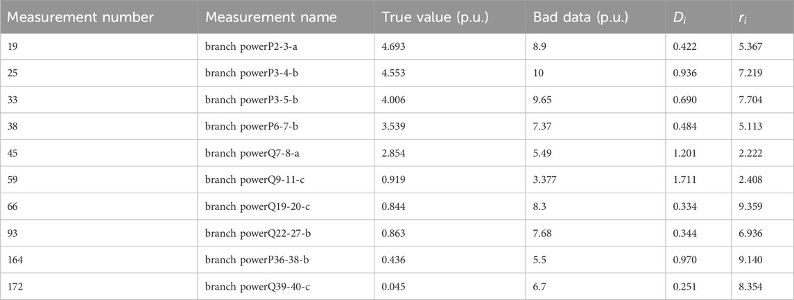
Table 3. Detail information of the bad data and the corresponding projection statistics and normalized residual values.
According to Table 4, among the 10 bad data, the projection statistical method effectively identified only 8 pcs bad data, while all other measurements with projection statistics values greater than 1 resulted in false alarms. Similarly, the maximum normalized residual method also failed to accurately identify the bad data. Therefore, both traditional statistical methods for bad data identification have certain limitations.

Table 4. Comparison of results of different identification methods.
4.3.2 Comparative analysis of single-stage and two-stage bad data identification methods
Due to the potential for misjudgments and missed detections by traditional statistical methods when multiple measurement bad data points are present in the system, these methods may not accurately identify measurement bad data. In contrast, the MILP bad data identification model used in the second stage can accurately identify all measurement bad data in the set identified by traditional methods when misjudgments or missed detections occur in the first stage. Therefore, in the first stage of this paper, all 265 lever measurements in the system were placed into a suspicious measurement set. The maximum normalized residual method was then used to identify the remaining 137 measurements, thereby validating the accuracy of the proposed bad data identification model and its efficiency compared to the single-stage model. Four sets of tests were conducted to compare the bad data identification method proposed in this paper with the traditional MINLP-based bad data identification method:
Test 1: Compression of the suspicious measurement set using the MILP-based two-stage bad data identification method proposed in this paper;
Test 2: Compression of the suspicious measurement set using the traditional MINLP-based two-stage bad data identification method;
Test 3: No compression of the suspicious measurement set, directly using the MILP-based single-stage bad data identification method;
Test 4: No compression of the suspicious measurement set, using the traditional MINLP-based single-stage bad data identification method.
Models were built for both methods in the GAMS optimization software, different solvers were called for calculation, and the results were compared and analyzed.
According to Table 5, for the modified IEEE-33 node test feeder case chosen in this paper, the two-stage model reduces the number of 0/1 integer variables and improves identification accuracy. However, for traditional MINLP-based bad data identification models, feasible solutions could not be obtained with most solvers, with correct results only achievable using the BONMIN solver. In contrast, the MILP-based bad data identification model achieved accurate identification results with most solvers. In terms of identification efficiency, even with the two-stage model, the MINLP identification model’s solving time reached the computational limit of 1,000 s, and the solver exited abnormally, indicating limited applicability. For the MILP-based bad data identification method, using the two-stage model, the SCIP solver improved solving efficiency by approximately 23 times, and the CPLEX solver achieved the highest efficiency, requiring only 0.546 s.

Table 5. Comparison of test results of different bad data identification methods.
5 Conclusion
To cope with the issue that existing traditional identification methods do not consider the nonlinear and discrete characteristics of on-load tap changers, making it difficult to achieve accurate and efficient identification of bad data., This paper proposes a MILP-based two stage bad data identification method. Detailed control characteristics of on-load tap changers are modelled, and a positive curvature quadratic penalty function is introduced to achieve fast tap normalization. In the first stage, leveraging projection statistics and maximum normalization residue methods effectively identifies leverage points and suspicious bad data, reduces the set of suspicious measurements. In the second stage, by linearizing nonlinear constraints and solving bad data identification model based on the MILP, the efficiency of the solution is greatly enhanced. The proposed model can achieve efficient and accurate identification of bad data, while ensuring optimal solutions by introducing penalty functions into the objective function for effective tap normalization.
Data availability statement
The original contributions presented in the study are included in the article, further inquiries can be directed to the corresponding author.
Author contributions
SH: Conceptualization, Funding acquisition, Methodology, Writing–original draft. CR: Formal Analysis, Investigation, Writing–original draft. MZ: Project administration, Resources, Writing–review and editing. LC: Software, Supervision, Writing–review and editing. YM: Validation, Visualization, Writing–review and editing. TZ: Validation, Visualization, Writing–review and editing.
Funding
The author(s) declare that financial support was received for the research, authorship, and/or publication of this article. This research was funded by State Grid Hebei Electric Power Co., Ltd. science and technology projects, grant number kj2023-076.
Conflict of interest
Authors SH, CR, and LC were employed by Economic and Technology Research Institute of State Grid Hebei Electric Power Co., Ltd.
The remaining authors declare that the research was conducted in the absence of any commercial or financial relationships that could be construed as a potential conflict of interest.
The authors declare that this study received funding from State Grid Hebei Electric Power Co.,Ltd. The funder had the following involvement in the study: the study design, collection, analysis, interpretation of data, and the writing of this article.
Publisher’s note
All claims expressed in this article are solely those of the authors and do not necessarily represent those of their affiliated organizations, or those of the publisher, the editors and the reviewers. Any product that may be evaluated in this article, or claim that may be made by its manufacturer, is not guaranteed or endorsed by the publisher.
References
Apland, J., and Sun, B. (2019). A Multi-Period, multiple objective, mixed integer programming, GAMS model for transit system planning
Baradar, M., and Hesamzadeh, M. R. (2014). A stochastic SOCP optimal power flow with wind power uncertainty. 1–5. doi:10.1109/PESGM.2014.6939790
Ghildyal, V., and Sahinidis, N. V. (2001). “Solving global optimization problems with baron,” in From Local to Global Optimization. Nonconvex Optimization and Its Applications. Editors A. Migdalas, P. M. Pardalos, and P. Värbrand (Boston, MA: Springer. doi:10.1007/978-1-4757-5284-7_10
Gupta, O. K., and Ravindran, A. (1985). Branch and bound experiments in convex nonlinear integer programming. Manage. Sci. 31 (12), 1533–1546. doi:10.1287/mnsc.31.12.1533
Handschin, E., and Kliokys, E. (1995). Transformer tap position estimation and bad data detection using dynamic signal modelling. IEEE T. Power Syst. 10 (2), 810–817. doi:10.1109/59.387921
Handschin, E., Schweppe, F. C., Kohlas, J., and Fiechter, A. (1975). Bad data analysis for power system state estimation. IEEE Trans. Power Apparatus Syst. 94 (2), 329–337. doi:10.1109/T-PAS.1975.31858
Huang, S. J., and Lin, J. M. (2004). Enhancement of anomalous data mining in power system predicting-aided state estimation. IEEE T. Power Syst. 19 (1), 610–619. doi:10.1109/TPWRS.2003.818726
Irving, M. R. (2008). Robust state estimation using mixed integer programming. IEEE T. Power Syst. 23 (3), 1519–1520. doi:10.1109/TPWRS.2008.926721
Ju, Y., and Huang, Y. (2023). State estimation for an AC/DC hybrid power system adapted to non-smooth characteristics. Power Syst. Prot. Control 51, 141–150. doi:10.19783/j.cnki.pspc.220368
Kia, R., Shahnazari-Shahrezaei, P., and Zabihi, S. (2016). Solving a multi-objective mathematical model for a multi-skilled project scheduling problem by CPLEX solver. IEEE, 1220–1224. doi:10.1109/IEEM.2016.7798072
Korres, G. N., Katsikas, P. J., and Contaxis, G. C. (2004). Transformer tap setting observability in state estimation. IEEE T. Power Syst. 19 (2), 699–706. doi:10.1109/TPWRS.2003.821629
Lin, Y., and Abur, A. (2018). A highly efficient bad data identification approach for very large scale power systems. IEEE T. Power Syst. 33 (6), 5979–5989. doi:10.1109/TPWRS.2018.2826980
Liu, Y., Zhang, N., Wang, Y., Yang, J., and Kang, C. (2019). Data-Driven power flow linearization: a regression approach. IEEE T. Smart Grid 10 (3), 2569–2580. doi:10.1109/TSG.2018.2805169
Maalouf, H., Jabr, R. A., and Awad, M. (2013). Mixed-integer quadratic programming based rounding technique for power system state estimation with discrete and continuous variables. Electr. Pow. Compo. Sys. 41 (5), 555–567. doi:10.1080/15325008.2012.755233
Mili, L., Cheniae, M. G., Vichare, N. S., and Rousseeuw, P. J. (1996). Robust state estimation based on projection statistics [of power systems]. IEEE T. Power Syst. 11, 1118–1127. doi:10.1109/59.496203
Nanchian, S., Majumdar, A., and Pal, B. (2017). Three-Phase state estimation using hybrid particle swarm optimization. IEEE T. Smart Grid. 8 (3), 1035–1045. doi:10.1109/TSG.2015.2428172
Shao, Z., Zhai, Q., and Guan, X. (2023). Physical-Model-Aided Data-Driven linear power flow model: an approach to address missing training data. IEEE T. Power Syst. 38 (3), 2970–2973. doi:10.1109/TPWRS.2023.3256120
Shiroi, M., and Hosseinie, S. H. (2008). “Observability and estimation of transformer tap setting with minimal PMU placement,” in IEEE power and energy society general meeting - conversion and delivery of electrical energy in the 21st century. Paper presented at the 2008. doi:10.1109/PES.2008.4596382
Teixeira, P. A., Brammer, S. R., Rutz, W. L., Merritt, W. C., and Salmonsen, J. L. (1992). State estimation of voltage and phase-shift transformer tap settings. IEEE T. Power Syst. 7 (3), 1386–1393. doi:10.1109/59.207358
Vigerske, S., and Gleixner, A. (2017). SCIP: global optimization of mixed-integer nonlinear programs in a branch-and-cut framework. Optim. Methods Softw. 33 (3), 563–593. doi:10.1080/10556788.2017.1335312
Zhao, J., and Mili, L. (2018). Vulnerability of the largest normalized residual statistical test to leverage points. IEEE T. Power Syst. 33 (4), 4643–4646. doi:10.1109/TPWRS.2018.2831453
Keywords: bad data identification, on-load-tap-changer, hyhrid data-physical driven, mixed integer linear programming, linearization
Citation: Hu S, Rong C, Zhang M, Chai L, Ma Y and Zhang T (2024) Bad data identification method considering the on-load tap changer model. Front. Energy Res. 12:1478834. doi: 10.3389/fenrg.2024.1478834
Received: 11 August 2024; Accepted: 26 September 2024;
Published: 11 October 2024.
Edited by:
Jinran Wu, Australian Catholic University, AustraliaReviewed by:
Yongqiang Kang, Lanzhou Jiaotong University, ChinaZhesen Cui, Changzhi University, China
Copyright © 2024 Hu, Rong, Zhang, Chai, Ma and Zhang. This is an open-access article distributed under the terms of the Creative Commons Attribution License (CC BY). The use, distribution or reproduction in other forums is permitted, provided the original author(s) and the copyright owner(s) are credited and that the original publication in this journal is cited, in accordance with accepted academic practice. No use, distribution or reproduction is permitted which does not comply with these terms.
*Correspondence: Shiyao Hu, ODQxMzQxOTcwQHFxLmNvbQ==