Application of deep forest algorithm incorporating seasonality and temporal correlation for wind speed prediction in offshore wind farm

Accurate prediction of wind speed is a prerequisite for the safe and accurate operation of wind power generation, however, WRF models typically do not produce sufficiently accurate wind speed predictions. This study proposed a Seasonal and Temporal Correlation - Deep Forest (STC-DF) model for offshore wind speed prediction. Different from traditional methods, the STC-DF model takes the advantages of the deep forest algorithm to automatically learn complex feature interactions without manual feature engineering. The model is designed to capture the seasonal and temporal characteristics of wind speed variations. To test the effectiveness of the proposed method, we applied the trained STC-DF model to an offshore wind farm in Hainan Province, China. Seven days of data from each season were selected for testing. The results show that the STC-DF model can effectively reduce the error caused by WRF forecast. The error index of the corrected wind speed reduced more than 40%, the accuracy of wind speed forecast increased 15%. And the method passed the multi-model comparison test and robustness experiment. These research results show that the STC-DF model has strong versatility and good correction ability, and is suitable for wind speed forecasting in different regions, which is a feasible method to improve the reliability of offshore wind power generation.

1 Introduction

Global climate change, energy supply and energy costs are becoming increasingly important to government authorities and society. As a result, countries are analyzing greater diversification of their sources of power generation towards renewable resources (Díaz and Soares, 2020). Renewable energy plays a key role in China’s energy strategy (Zhang and Wang, 2022). Wind energy has the prospect of being an alternative source of energy for power generation and, unlike fossil fuels, it reduces the amount of carbon dioxide emitted into the atmosphere. This intermittent nature of energy has led to the development and improvement of wind forecasting systems (Pereyra-castro and Caetano, 2022). China is a vast country with a total of 300 million kilowatts of wind energy that can be exploited annually in the country (Qian et al., 2016). As the development of onshore wind power in China is already relatively saturated, the development of offshore wind power will become an important means of addressing the fundamental interplay between future energy mix and supply patterns (Chen and Lin, 2022). The continental coastline is 18,400 km long (Zhang and Wang, 2022), with an island coastline of 14,247 km and a total coastline length of more than 32,600 km, there is great potential for the development of offshore wind resources. After more than two decades of industrialization and development, the offshore wind power industry has gradually moved from the demonstration stage to the commercialization stage, and is receiving more and more attention from national governments (Soares-Ramos et al., 2020; Irena, 2016). Wind speed prediction can effectively predict the future wind strength and power output of wind turbines, which provides data support for wind power operators to design wind turbine on-line strategies and maintenance plans, and can improve the competitiveness of wind power products in the energy market. Therefore, the accurate prediction of wind speed in offshore wind farms is of vital importance for the development of renewable energy.

Wind speed prediction today can be categorized into two schemes: data-driven schemes and physical schemes. Data-driven methods are currently a hot area for researchers in the field of wind power. It uses the intrinsic relationship of multi-source meteorological data to build mathematical and statistical models (Yang et al., 2005; Zeng et al., 2012), machine learning models (Liu et al, 2021a; Cassola and Burlando, 2012) and hybrid models (Papaefthymiou and Klockl, 2008; Liu et al, 2021b) and other prediction models to predict wind speed. However, the prediction step provided by traditional statistical model is difficult to meet the needs of China’s wind farms (Zheng et al., 2011). Physical methods can be subdivided into two categories: numerical weather prediction methods (NWP) and spatial correlation methods (Zhang et al., 2020). The NWP method uses weather forecast data such as temperature, pressure, surface roughness, and obstacles to predict wind power, which is suitable for predicting wind power in power plants because it describes atmospheric motion without the need for large amounts of historical data (Yu et al., 2019). Currently, there are many different physical methods for wind speed prediction such as high-resolution limited area model (HIRLAM) (Landberg, 1999)、Mesoscale Model5 (MM5) (Salcedo-Sanz et al., 2009) and Weather Research and Forecasting (WRF) model (Zhao et al., 2017). Among them, the WRF model can provide ultra-high resolution and its Large Eddy Simulations (LES) scheme can effectively simulate the atmospheric motions of wind farms due to the fact that it is favored by wind farm operators (Prósper et al., 2019). However, numerical weather prediction results in large errors due to imperfect physical parameterization schemes, low resolution, and inaccurate topography. Due to the errors in wind speed prediction, it is difficult to meet the needs of wind farms in China (Xiong et al., 2023; Chang et al., 2015; Hu, 2016; Zhang et al., 2013). Meanwhile, physical algorithms have advantages in long-term forecasting. However, they require a lot of computational time and are not suitable for short-term forecasting (Liu et al., 2015). Therefore, a single physical model needs to be assisted by other methods to realize high-precision wind power prediction in practical engineering applications.

Popular data-driven techniques mainly include signal processing, machine learning and information fusion (Zhang et al., 2023). In recent years, there has been a gradual increase in the research of using multiple meta-learners to combine to form highly interpretable models (Jiang et al., 2024; Liu et al., 2023; Liu et al., 2024a; Liu et al., 2024b), and the combination of signal processing and machine learning to construct hybrid models for wind speed prediction has become a hot topic (Jiang et al., 2023; Zhang et al., 2024). Literature (Chen et al., 2022) proposed a new wind speed prediction model that combines CEEMDAN, VMD, and LSTM. The error model combining VMD and LSTM can extract deeper features and improve the correction effect of the model. Zhang and Liu (2022) focused on post-processing the error signals and proposed an ELM-ICEEMDAN-ARIMA hybrid model for short-term wind speed forecasting. Zhou et al. (2023) proposed a hybrid prediction method for wind speed combining machine learning algorithms such as variational modal decomposition (VMD), principal component analysis (PCA) and random forest (RF). Xiong et al. (2023) extracted the wind speed fluctuation features and labeled them using the fluctuation stable day model, and combined them with BO and LSTM for wind speed prediction. Establishing a suitable AI hybrid model to predict wind speed will be of great significance for the proper operation of wind farms.

Deep Forest is a cascade random forest algorithm based on deep models (Mao and Li, 2024), Compared to deep neural networks, it has fewer hyperparameters, lower data requirements, adaptive model complexity, and good robustness and generalization capabilities. Therefore, it is widely used in target recognition, image processing, text recognition, fault diagnosis, network intrusion detection, medical diagnosis, and other fields (Zhou and Feng, 2019). Mao introduced the idea of weight distribution in the cascade forest construction stage and proposed an improved DF algorithm based on information theory. This algorithm evaluates training samples to decide whether they enter the next level of training, thereby reducing the number of samples and improving the model’s parallel training efficiency (Mao et al., 2022). Yin et al. (2020) applied the deep forest regression method to short-term load forecasting in power systems. The results showed that the default configuration parameters of the deep forest regression could improve short-term prediction accuracy and reduce the impact of experience on hyperparameter configuration of deep learning models. Liu et al. (2020) proposed a combined deep forest-based prediction model for short-term wind speed prediction. Wang et al. (2021) combined empirical modal decomposition and deep forests for wind speed prediction. Although the direct application of deep forests in wind speed prediction is not yet widespread, integrated learning methods have shown good potential in this field. Deep forest, as a powerful integrated learning algorithm, is expected to play a greater role in future wind speed prediction research.

However, offshore wind farms are subject to various factors due to their unique topographical characteristics, resulting in poor wind speed stability. Wind speed prediction models will face greater challenges and need to be updated more frequently to adapt to the changes brought about by different influencing factors. In summary, the field of wind speed prediction has the following issues to be addressed:

(1) The influencing factors of wind speed prediction methods are not comprehensively considered. Wind speed exhibits seasonality, with variations in speed and volatility across different seasons. Seasonal factors have a significant impact on wind speed sequences.

(2) The feature factors input into wind speed prediction models are highly limited. Traditional prediction models only use wind speed data as input, without considering the impact of meteorological elements on wind speed variations and the historical autocorrelation of the input data. Therefore, it is difficult to capture subtle changes and short-term fluctuations in the data.

To address the above issues, we propose a model named Seasonal and Temporal Correlation - Deep Forest (STC-DF), which considers the impact of seasonal characteristic changes and temporal correlation of wind speed variations on wind speed prediction for offshore wind farms. The contributions of this study to the above two issues are as follows:

(1) Seasonal Training Correction Model: By extracting the main features from various meteorological elements of NWP predictions for each season, the input feature factors of the model are enriched. Appropriate models are selected for training and prediction on specific data to more accurately capture the randomness, intermittency, and volatility characteristics of actual wind speed.

(2) Incorporating Data Differencing: By including adjacent differences in predicted wind speed, trends and seasonality are eliminated, and lag effects are reduced. This reveals hidden patterns and relationships in the original time series, providing the model with more useful features and thereby improving prediction performance.

Through multi-model comparison test and robustness experiment, the effectiveness and generalizability of this method for wind speed prediction correction have been verified.

2 Data and methods

2.1 Data

The target wind farm for this study is an offshore wind farm in Hainan Province, and the wind speed data used are system derived wind speeds at the wind farm level with a time resolution of 15 min. The forecast data were generated by the WRF system, and since the turbine hub height is 70 m, 70-m wind speed (WS_pre), 2-m temperature (T), 2-m surface pressure (PRS), precipitation (PRE) and 2-m humidity (RH) were selected as input features for the correcting model. Connect all the data according to the timestamp and perform preprocessing such as fusion and cleaning. The data of the target wind farm in 2023 was selected as the study data. In the field of meteorology, seasons are usually divided according to the change of temperature patterns: spring (March-May), summer (June-August), autumn (September-November) and winter (December-February) (Linacre, 1992). The data from the last 7 days of each season was selected as the test set and the rest of the data was used as the training set.

2.2 Method

2.2.1 WRF model

In this study, the WRF regional mesoscale numerical prediction model is used to simulate the offshore wind farm, and the WRF model adopts a three-layer nested grid structure, with the grid numbers of 180 × 190, 100 × 90, and 110 × 110, and the grid spacings of 27 km, 9 km, and 3 km, respectively, and the initial field and boundary conditions are based on the Global Weather Forecast (GWF) data provided by the National Centers for Environmental Prediction (NCEP). The initial field and boundary conditions are based on the global weather forecast data provided by the National Centers for Environmental Prediction (NCEP) of the United States, with a temporal resolution of 7 days and a spatial resolution of 1° × 1°. Figure 1 shows the basic operation of the WRF model. In the WRF model setup, the physical process parameterization schemes, such as the Yonsei University boundary layer parameterization scheme (Hong et al., 2006), the Grell-Freitas convective parameterization scheme (Grell and Freitas, 2014), the RRTMG short- and long-wavelength radiation scheme (Iacono et al., 2008), and the Noah surface process scheme (Chen and Dudhia, 2001), are used. The time integration is based on the Runge-Kutta 3rd order scheme, and the computational time step is adaptively adjusted according to the CFL conditions.

Figure 1

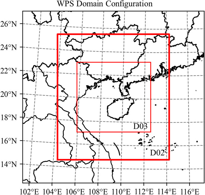
Figure 1. WRF model simulation area.

2.2.2 Deep forest

Deep Forest (DF) (Zhou and Feng, 2019) is an integrated learning algorithm based on deep learning. The method stacks multiple random forest models together to form a deep network structure, and uses the output of each layer of random forest as the input features of the next layer. Specifically, Deep Forest consists of the following steps:

Step1: gcForest employs a cascade structure to enable level-by-level processing, where each level of the cascade receives feature information processed by its predecessor level and outputs the results of its processing to the next level.

Step2: Each level is a collection of decision tree forests, i.e., a collection of sets, including different types of forests to encourage diversity. Each forest contains multiple trees, where the number of trees is a hyperparameter.

Step3: Each forest processes raw features to generate class vectors and augmented feature vectors, which are then used to train the forest in the next cascade. This process is implemented by multi-granularity scanning, where the original features are scanned using a sliding window to produce feature vectors of different sizes.

Step4: Each forest generates class vectors through k-fold cross-validation. During training, cross-validation is used to evaluate the performance of the entire cascade and terminate the training if necessary to prevent overfitting.

Step5: The number of classes in the cascade is automatically determined by estimating the performance of the entire cascade on the validation set, and the training process is terminated if there is no significant performance gain.

Unlike traditional integrated learning methods, Deep Forest is able to automatically learn the complex interactions between features without relying on manually designed feature engineering. In addition, the method has low computational complexity, is not easy to overfitting, and shows excellent classification performance on multiple benchmark datasets. The structure of Deep Forest is shown in Figure 2.

Figure 2

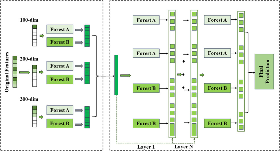
Figure 2. The structure of Deep Forest algorithm.

2.2.3 Seasonal and temporal correlation - deep forest model

In order to better capture the relationship between seasonality, temporal correlation and meteorological factors in wind speed prediction problems, we propose to use STC-DF model to achieve better performance in wind speed prediction tasks. The model consists of the following main components:

(1) Seasonal sub-model: the year is divided into four seasons, and four sub-models are trained to capture the characteristics of wind speed changes in different seasons.

(2) Integration time-series features: In addition to the conventional features of temperature, humidity, pressure and other meteorological elements, the difference between the wind speed (WS_diff) at the previous moment and the current moment was also added to reflect the correlation in the time series.

(3) Deep forest model: The deep forest algorithm was used as the base model, and its powerful feature learning and non-linear modelling capabilities were used to predict wind speed.

The flowchart of the proposed hybrid model is given in Figure 3. The STC-DF model is carried out in the following three steps:

Step 1: Model training. Four sub-models were trained for different seasons. For each sub-model, the corresponding features were extracted and trained.

Step 2: Model predictions. Wind speed predictions were made by first identifying the season based on the current time and then using the appropriate sub-model to make the predictions. The predictions will reflect both seasonal and temporal correlations.

Step 3: Results evaluation. The accuracy of the model was evaluated by the wind speed evaluation index. In order to verify the validity as well as the generalizability of the model, multi-model comparison experiment and robustness experiment will be conducted for the model.

Figure 3

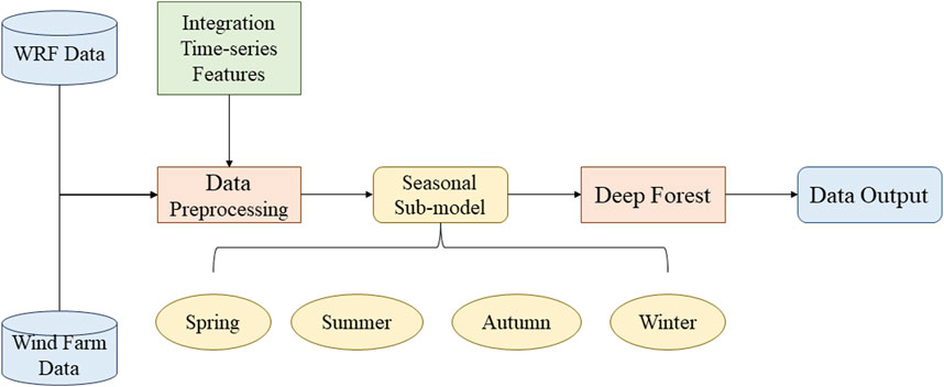
Figure 3. The flowchart of the proposed hybrid model.

Through the integration of the above seasonal sub-models, time-series features and meteorological element features, the STC-DF Model is able to better learn the intrinsic law of wind speed change, and thus improve the accuracy and reliability of wind speed prediction.

2.2.4 Error analysis method

In order to evaluate the correction effect of the model, four error metrics, namely, Root Mean Square Errors (RMSE, Equation 1), Relative Root Mean Square Errors (rRMSE, Equation 2), Forecast Accuracy (FA, Equation 3) of wind speed, and Correlation Coefficient R (Equation 4), are chosen to measure the correction effect in this paper. The formulas for the error metrics are as follows:

$\mathit{R}\mathit{M}\mathit{S}\mathit{E}=\sqrt{\frac{\mathbf{1}}{\mathit{n}}{\displaystyle \sum _{\mathit{i}-\mathbf{1}}^{\mathit{n}}}{\left(\widehat{{\mathit{y}}_{\mathit{i}}}-{\mathit{y}}_{\mathit{i}}\right)}^{\mathbf{2}}}(1)$

$\mathit{r}\mathit{R}\mathit{M}\mathit{S}\mathit{E}=\frac{\sqrt{\frac{\mathbf{1}}{\mathit{n}}{\displaystyle \sum _{\mathit{i}=\mathbf{1}}^{\mathit{n}}}{\left({\mathit{y}}_{\mathit{i}}-{\widehat{\mathit{y}}}_{\mathit{i}}\right)}^{\mathbf{2}}}}{\frac{\mathit{i}}{\mathit{n}}{\displaystyle \sum _{\mathit{i}=\mathbf{1}}^{\mathit{n}}}{\mathit{y}}_{\mathit{i}}}\times \mathbf{100}\%(2)$

$\mathit{F}\mathit{A}=\frac{{\mathit{N}}_{\mathit{r}}}{{\mathit{N}}_{\mathit{f}}}\times \mathbf{100}\%(3)$

$\mathit{R}=\frac{{\displaystyle \sum _{\mathit{i}=\mathbf{1}}^{\mathit{n}}}\left({\mathit{x}}_{\mathit{i}}-\overline{\mathit{x}}\right)\left({\mathit{y}}_{\mathit{i}}-\overline{\mathit{y}}\right)}{\sqrt{{\displaystyle \sum _{\mathit{i}=\mathbf{1}}^{\mathit{n}}}{\left({\mathit{x}}_{\mathit{i}}-\overline{\mathit{x}}\right)}^{\mathbf{2}}}\sqrt{{\displaystyle \sum _{\mathit{i}=\mathbf{1}}^{\mathit{n}}}{\left({\mathit{y}}_{\mathit{i}}-\overline{\mathit{y}}\right)}^{\mathbf{2}}}}(4)$

where $\widehat{y_i}$ represents the $i$ th predicted value, $y_i$ denotes the $i$ th observation, $n$ is the total number of time samples, and $\overline{y}$ is the average of the observed values. Here, $N_r$ stands for the number of samples with an absolute deviation of the wind speed forecast less than 1 m/s, while $N_f$ is the number of samples forecasted.

3 Results and discussion

3.1 Result of seasonal sub-models

Four seasonal sub-models were developed using the above methodology to forecast corrected wind speeds for each of the four seasons of the offshore wind farm. The correlations between the variables of the test set in the seasonal sub-models are given in Figure 4, and the correlations between the observed wind speed and each of the variables are different for each season. Since DF possesses a natural anti overfitting property, i.e., it comes with a cross-validation process. It can achieve to a better result without any parameter tuning. There is a strong correlation between observed wind speed and WRF predicted wind speed in both spring and summer. Except in winter, the correlation between each variable and the observed wind speed is strong, and the positive and negative values of the correlation will change significantly with the change of season. It can be seen that seasonal sub-model training for wind speed prediction correction is very necessary.

Figure 4

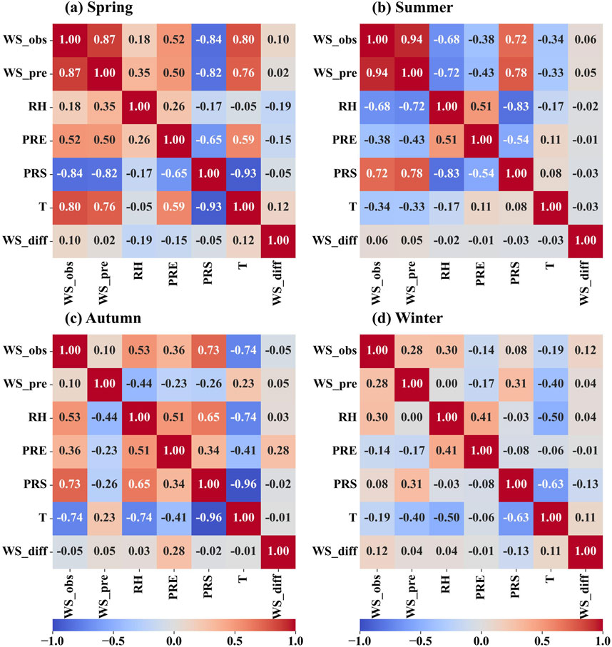
Figure 4. Correlation plots between the variables of the seasonal sub-models. (A) Spring, (B) Summer, (C) Aututmn, (D) Winter.

The forecast impact of the seasonal sub-models was assessed and compared with that of WRF (Table 1). The STC-DF model led to varying degrees of improvement in wind speed error correction across different seasons. The original WRF exhibited the largest and smallest prediction errors in summer and winter, respectively. The RMSE decreased by 30.74%, 30.24%, 32.99%, and 34.65% for the four seasons, all surpassing a 30% reduction. In autumn and winter, R showed the most significant increase, from 0.1 to 0.72 and from 0.28 to 0.72, respectively.

Table 1

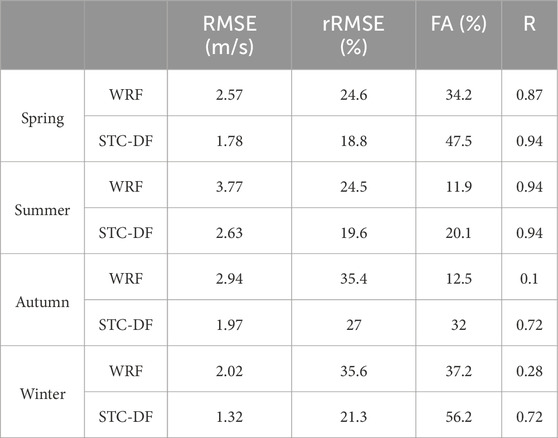
Table 1. Evaluation of the seasonal sub-models forecast effect.

After counting the various error indicators of the seasonal sub-models, the prediction results are visualized. As shown in Figure 5 time series comparison chart, it can be intuitively seen that the seasonal sub-models improved the inaccuracy of WRF forecast wind speed in different degrees, making the corrected wind speed closer to the observed wind speed as a whole. Moreover, the models have the best correction effect in the middle of the wind speed, and the performance will be reduced when the wind speed is very high or very low. By observing the overall distribution of wind speed in the test set in the seasonal sub-models (Figure 6), it is not difficult to find that the wind speed forecast in summer is overall high, while the other three seasonal forecasts are overall low. Through the correction of the STC-DF model, the forecast deviation of the four seasons is reduced, and the quantiles are closer to the true values.

Figure 5

Figure 5. Comparison of observed wind speed, WRF forecast wind speed and STC-DF forecast wind speed time series in the seasonal sub-models.

Figure 6

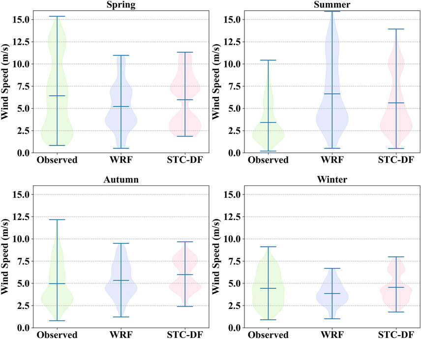
Figure 6. Distribution of wind speed in the seasonal sub-models.

3.2 Result of STC-DF model

The corrected results of the seasonal sub-models were summarized to obtain the overall test set correction results. By comparing the regression scatter density plots of the forecast results from the WRF model and the STC-DF model (Figure 7), it can be seen that the forecast values of the STC-DF model are more convergent than those of the WRF model, with fewer outliers and a more concentrated distribution of data points. The forecast wind speed of the STC-DF model compared with that of the WRF model shows that the RMSE decreased from 2.45 m/s to 1.42 m/s, the rRMSE decreased from 15.5% to 10.4%. And the FA increased from 24% to 39%, R increased from 0.83 to 0.89. The error metric RMSE is reduced by 42.04%, which shows that the STC-DF model has considerable effect on wind speed correction.

Figure 7

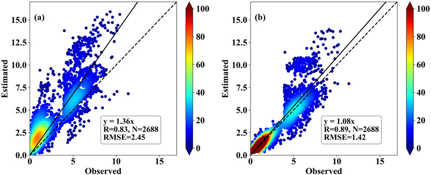
Figure 7. Regression scatter plot of predicted wind speed. (A) WRF model, (B) STC-DF model.

3.3 Multi-model comparison test

In order to verify the effectiveness of the STC-DF model, we chose the DF, RF, XGBoost, LightGBM, MLP and LSTM algorithms for the wind speed data of the target wind farm to conduct a multi-model comparison test. The same data were chosen as the training set and test set in the experiment. The error values of the experimental results are given in Table 2. After comparison, the STC-DF model has lower RMSE and rRMSE, higher FA and R. The hybrid model proposed in this study can successfully reduce the errors brought by the WRF model and shows excellent performance.

Table 2

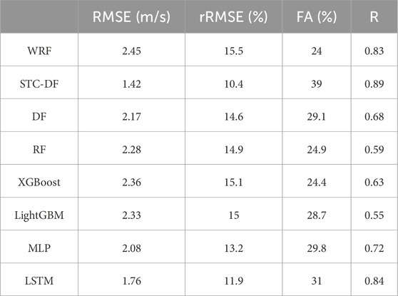
Table 2. The result of multi-model comparison test.

3.4 Robustness experiment

In order to test the generality of the proposed method in this study, we applied the trained STC-DF model to an offshore wind farm in Guangdong Province for robustness experiment. Seven days of data are randomly selected from each season for the test, and the error distributions of the wind speed forecasted by the WRF model and those forecasted by the STC-DF model are shown in Figure 8. The method in this paper can effectively reduce the errors caused by WRF forecasts, and the outliers of predicted wind speed are reduced, with different degrees of improvement in each season. The RMSE of the sub-model forecast data in all seasons decreased from 2.78 m/s to 1.86 m/s, the FA increased from 25.4% to 42%, and the R increased from 0.57 to 0.8. The results fully demonstrate that the STC-DF model has strong generality, and it also has a better correction ability for wind speed of wind farm in different regions.

Figure 8

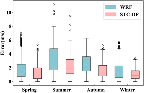
Figure 8. Boxplot distribution of errors for seasonal sub-models.

4 Conclusion and discussion

4.1 Conclusion

In order to solve the problem of feature extraction limitations and incomplete consideration of wind speed influence factors in wind speed correction methods, this study proposed a correction method based on deep forest algorithm integrating seasonal and temporal correlation. The proposed STC-DF model considered the seasonal difference and time correlation of wind speed, combined meteorological data and wind speed difference, and showed good performance in wind speed correction of offshore wind farms in Hainan Province and Guangdong Province. Compared with WRF data, the error index of the corrected wind speed reduced more than 40%, the accuracy of wind speed forecast increased 15%. In summary, the STC-DF model can effectively reduce the error caused by the WRF model forecast, improve the accuracy of the forecast, and contribute to the stable operation of the offshore wind farm, so as to improve the economic benefits of wind power.

4.2 Discussion

Through the robustness experiment, it is easy to see that the STC-DF model performed well for wind speed prediction in different offshore wind farms. However, due to the lack of data information of wind farms in different terrains, it is uncertain about the performance of the model in different terrain wind farms, such as mountain wind farms and plateau wind farms. In addition, since the wind farm data is only for 1 year, the time series input into the seasonal sub-model is not long enough, and the model still has room for improvement. The model is not effective in forecasting the extreme value of wind speed, and the amount of data input to the model will be increased in the future to get better prediction results. In the future research, stabilization models adapted to the characteristics of different wind farms or the number of hidden features to be mined according to different types of wind farms will also be considered.

Data availability statement

The datasets presented in this article are not readily available because The data that has been used is confidential. Requests to access the datasets should be directed to Weixiao Lu, luweixiao00@163.com.

Author contributions

HF: Data curation, Investigation, Writing–original draft. SL: Software, Writing–review and editing. JZ: Writing–review and editing, Validation. WL: Methodology, Visualization, Writing–original draft.

Funding

The author(s) declare that no financial support was received for the research, authorship, and/or publication of this article.

Conflict of interest

Authors HF, SL, and JZ were employed by Hainan Shenneng New energy Co., LTD.

The remaining author declares that the research was conducted in the absence of any commercial or financial relationships that could be construed as a potential conflict of interest.

Publisher’s note

All claims expressed in this article are solely those of the authors and do not necessarily represent those of their affiliated organizations, or those of the publisher, the editors and the reviewers. Any product that may be evaluated in this article, or claim that may be made by its manufacturer, is not guaranteed or endorsed by the publisher.

References

Cassola, F., and Burlando, M. (2012). Wind speed and wind energy forecast through Kalman filtering of Numerical Weather Prediction model output. Appl. energy 99, 154–166. doi:10.1016/j.apenergy.2012.03.054

CrossRef Full Text | Google Scholar

Chang, J., Peng, X., Fan, G., and Che, Y. (2015). Error calibration of numerical weather prediction with historical data. Acta. Meteorologica. Sinica. (2), 341–354. doi:10.11676/qxxb2015.021

CrossRef Full Text | Google Scholar

Chen, C., Zhao, X., Bi, G., Xie, X., Gao, J., and Luo, Z. (2022). SSA-Res-GRU short-term wind speed prediction model based on multi-model decomposition. Power Grid Technol. 46 (08), 2975–2985. doi:10.13335/j.1000-3673.pst.2021.2510

CrossRef Full Text | Google Scholar

Chen, F., and Dudhia, J. (2001). Coupling an advanced land surface–hydrology model with the Penn State–NCAR MM5 modeling system. Part I: model implementation and sensitivity. Mon. weather Rev. 129 (4), 569–585. doi:10.1175/1520-0493(2001)129<0569:caalsh>2.0.co;2

CrossRef Full Text | Google Scholar

Chen, Y., and Lin, H. (2022). Overview of the development of offshore wind power generation in China. Sustain. energy Technol. assessments 53, 102766. doi:10.1016/j.seta.2022.102766

CrossRef Full Text | Google Scholar

Díaz, H., and Soares, C. G. (2020). Review of the current status, technology and future trends of offshore wind farms. Ocean. Eng. 209, 107381. doi:10.1016/j.oceaneng.2020.107381

CrossRef Full Text | Google Scholar

Grell, G. A., and Freitas, S. R. (2014). A scale and aerosol aware stochastic convective parameterization for weather and air quality modeling. Atmos. Chem. Phys. 14 (10), 5233–5250. doi:10.5194/acp-14-5233-2014

CrossRef Full Text | Google Scholar

Hong, S. Y., Noh, Y., and Dudhia, J. (2006). A new vertical diffusion package with an explicit treatment of entrainment processes. Mon. weather Rev. 134 (9), 2318–2341. doi:10.1175/mwr3199.1

CrossRef Full Text | Google Scholar

Hu, B. (2016). Experimental application of a probability method in predicting typhoon gusts on coastal islands. Meteorological Sci. Technol. 44 (02), 246–251. doi:10.19517/j.1671-6345.2016.02.013

CrossRef Full Text | Google Scholar

Iacono, M. J., Delamere, J. S., Mlawer, E. J., Shephard, M. W., Clough, S. A., and Collins, W. D. (2008). Radiative forcing by long-lived greenhouse gases: calculations with the AER radiative transfer models. J. Geophys. Res. Atmos. 113 (D13). doi:10.1029/2008jd009944

CrossRef Full Text | Google Scholar

Irena (2016). “Innovation outlook: off shore wind.” Abu Dhabi: International Renewable Energy Agency.

Google Scholar

Jiang, P., Liu, Z., Abedin, M. Z., Wang, J., Yang, W., and Dong, Q. (2024). Profit-driven weighted classifier with interpretable ability for customer churn prediction. Omega 125, 103034. doi:10.1016/j.omega.2024.103034

CrossRef Full Text | Google Scholar

Jiang, Z., Che, J., He, M., and Yuan, F. (2023). A CGRU multi-step wind speed forecasting model based on multi-label specific XGBoost feature selection and secondary decomposition. Renew. Energy 203, 802–827. doi:10.1016/j.renene.2022.12.124

CrossRef Full Text | Google Scholar

Landberg, L. (1999). Short-term prediction of the power production from wind farms. J. wind Eng. industrial Aerodynamics 80 (1-2), 207–220. doi:10.1016/s0167-6105(98)00192-5

CrossRef Full Text | Google Scholar

Linacre, E. (1992). Climate data and resources: a reference and guide.

Google Scholar

Liu, H., Tian, H. Q., Liang, X. F., and Li, Y. F. (2015). Wind speed forecasting approach using secondary decomposition algorithm and Elman neural networks. Appl. Energy 157, 183–194. doi:10.1016/j.apenergy.2015.08.014

CrossRef Full Text | Google Scholar

Liu, M. D., Ding, L., and Bai, Y. L. (2021b). Application of hybrid model based on empirical mode decomposition, novel recurrent neural networks and the ARIMA to wind speed prediction. Energy Convers. Manag. 233, 113917. doi:10.1016/j.enconman.2021.113917

CrossRef Full Text | Google Scholar

Liu, X., Lin, Z., and Feng, Z. (2021a). Short-term offshore wind speed forecast by seasonal ARIMA-A comparison against GRU and LSTM. Energy 227, 120492. doi:10.1016/j.energy.2021.120492

CrossRef Full Text | Google Scholar

Liu, Z., De Bock, K. W., and Zhang, L. (2024a). Explainable profit-driven hotel booking cancellation prediction based on heterogeneous stacking-based ensemble classification. Eur. J. Operational Res. doi:10.1016/j.ejor.2024.08.026

CrossRef Full Text | Google Scholar

Liu, Z., Jiang, P., Wang, J., Du, Z., Niu, X., and Zhang, L. (2023). Hospitality order cancellation prediction from a profit-driven perspective. Int. J. Contemp. Hosp. Manag. 35 (6), 2084–2112. doi:10.1108/IJCHM-06-2022-0737

CrossRef Full Text | Google Scholar

Liu, Z., Jiang, P., Zhang, L., and Niu, X. (2020). A combined forecasting model for time series: application to short-term wind speed forecasting. Appl. Energy 259, 114137. doi:10.1016/j.apenergy.2019.114137

CrossRef Full Text | Google Scholar

Liu, Z., Zhang, Y., Abedin, M. Z., Wang, J., Yang, H., Gao, Y., et al. (2024b). Profit-driven fusion framework based on bagging and boosting classifiers for potential purchaser prediction. J. Retail. Consumer Serv. 79, 103854. doi:10.1016/j.jretconser.2024.103854

CrossRef Full Text | Google Scholar

Mao, Y., Geng, J., and Chen, L. (2022). Parallel deep forest algorithm improved by combining information theory. Comput. Eng. Appl. 58 (07), 106–115. doi:10.3778/j.issn.1002-8331.2103-0019

CrossRef Full Text | Google Scholar

Mao, Y., and Li, W. (2024). Parallel deep forest algorithm based on mutual information and fusion weighting. Comput. Appl. Res. 41 (02), 473–481. doi:10.19734/j.issn.1001-3695.2023.05.0240

CrossRef Full Text | Google Scholar

Papaefthymiou, G., and Klockl, B. (2008). MCMC for wind power simulation. IEEE Trans. energy Convers. 23 (1), 234–240. doi:10.1109/tec.2007.914174

CrossRef Full Text | Google Scholar

Pereyra-castro, K., and Caetano, E. (2022). Wind-ramp predictability. Atmosphere 13 (3), 453. doi:10.3390/atmos13030453

CrossRef Full Text | Google Scholar

Prósper, M. A., Otero-Casal, C., Fernández, F. C., and Miguez-Macho, G. (2019). Wind power forecasting for a real onshore wind farm on complex terrain using WRF high resolution simulations. Renew. energy 135, 674–686. doi:10.1016/j.renene.2018.12.047

CrossRef Full Text | Google Scholar

Qian, Z., Pei, Y., Cao, L., Wang, J., and Jing, B. (2016). Review of wind power forecasting method. High. Volt. Eng. 42 (04), 1047–1060. doi:10.13336/j.1003-6520.hve.20160405021

CrossRef Full Text | Google Scholar

Salcedo-Sanz, S., Pérez-Bellido, Á. M., Ortiz-García, E. G., Portilla-Figueras, A., Prieto, L., and Paredes, D. (2009). Hybridizing the fifth generation mesoscale model with artificial neural networks for short-term wind speed prediction. Renew. Energy 34 (6), 1451–1457. doi:10.1016/j.renene.2008.10.017

CrossRef Full Text | Google Scholar

Soares-Ramos, E. P., de Oliveira-Assis, L., Sarrias-Mena, R., and Fernández-Ramírez, L. M. (2020). Current status and future trends of offshore wind power in Europe. Energy 202, 117787. doi:10.1016/j.energy.2020.117787

CrossRef Full Text | Google Scholar

Wang, Y., Wang, J., Wei, X., and Hurtado-Pérez, E. (2021). A cascade hybrid PSO feed-forward neural network model of a biomass gasification plant for covering the energy demand in an AC microgrid. Energy Convers. Manag. 232, 113896. doi:10.1016/j.enconman.2021.113896

CrossRef Full Text | Google Scholar

Xiong, X., Zou, R., Sheng, T., Zeng, W., and Ye, X. (2023). An ultra-short-term wind speed correction method based on the fluctuation characteristics of wind speed. Energy 283, 129012. doi:10.1016/j.energy.2023.129012

CrossRef Full Text | Google Scholar

Yang, X., Xiao, Y., and Chen, S. (2005). Wind speed and generated power forecasting in wind farm. Proceedings-Chinese Soc. Electr. Eng. 25 (11), 1. doi:10.1360/biodiv.050028

CrossRef Full Text | Google Scholar

Yin, L., Sun, Z., Gao, F., and Liu, H. (2020). Deep forest regression for short-term load forecasting of power systems. IEEE Access 8, 49090–49099. doi:10.1109/access.2020.2979686

CrossRef Full Text | Google Scholar

Yu, R., Gao, J., Yu, M., Lu, W., Xu, T., Zhao, M., et al. (2019). LSTM-EFG for wind power forecasting based on sequential correlation features. Future Gener. Comput. Syst. 93, 33–42. doi:10.1016/j.future.2018.09.054

CrossRef Full Text | Google Scholar

Zeng, C., Ye, L., and Zhao, Y. (2012). Spatial model for short term wind power prediction considering wake effects. Power Syst. Prot. Control 40 (24), 59–142.

Google Scholar

Zhang, C., Luo, L., Yang, Z., Du, B., Zhou, Z., Wu, J., et al. (2024). Flexible method for estimating the state of health of lithium-ion batteries using partial charging segments. Energy 295, 131009. doi:10.1016/j.energy.2024.131009

CrossRef Full Text | Google Scholar

Zhang, C., Zhao, S., Yang, Z., and He, Y. (2023). A multi-fault diagnosis method for lithium-ion battery pack using curvilinear Manhattan distance evaluation and voltage difference analysis. J. Energy Storage 67, 107575. doi:10.1016/j.est.2023.107575

CrossRef Full Text | Google Scholar

Zhang, J., and Liu, Z. (2022). Ultra short term wind speed interval prediction based on a hybrid model. Power Syst. Prot. Control 50 (22), 49–58. doi:10.19783/j.cnki.pspc.220241

CrossRef Full Text | Google Scholar

Zhang, J., and Wang, H. (2022). Development of offshore wind power and foundation technology for offshore wind turbines in China. Ocean. Eng. 266, 113256. doi:10.1016/j.oceaneng.2022.113256

CrossRef Full Text | Google Scholar

Zhang, Y., Guo, Z., Lin, Y., and Chi, D. (2013). Predictive capacity of mesoscale model for short-range wind speed forecasting at wind power farm. Chin. J. Atmos. Sci. 37 (04), 955–962. doi:10.3878/j.issn.1006-9895.2012.12092

CrossRef Full Text | Google Scholar

Zhang, Y., Li, Y., and Zhang, G. (2020). Short-term wind power forecasting approach based on Seq2Seq model using NWP data. Energy 213, 118371. doi:10.1016/j.energy.2020.118371

CrossRef Full Text | Google Scholar

Zhao, J., Guo, Y., Xiao, X., Wang, J., Chi, D., and Guo, Z. (2017). Multi-step wind speed and power forecasts based on a WRF simulation and an optimized association method. Appl. energy 197, 183–202. doi:10.1016/j.apenergy.2017.04.017

CrossRef Full Text | Google Scholar

Zheng, Z. W., Chen, Y. Y., Huo, M. M., and Zhao, B. (2011). An overview: the development of prediction technology of wind and photovoltaic power generation. Energy Procedia 12, 601–608. doi:10.1016/j.egypro.2011.10.081

CrossRef Full Text | Google Scholar

Zhou, S., Gao, Y., Duan, Z., Xi, X., and Li, Y. (2023). A robust error correction method for numerical weather prediction wind speed based on Bayesian optimization, Variational Mode Decomposition, Principal Component Analysis, and Random Forest: VMD-PCA-RF. EGUsphere 2023, 1–37. doi:10.5194/egusphere-2023-945

CrossRef Full Text | Google Scholar

Zhou, Z. H., and Feng, J. (2019). Deep forest. Natl. Sci. Rev. 6 (1), 74–86. doi:10.1093/nsr/nwy108

PubMed Abstract | CrossRef Full Text | Google Scholar