Forecasting day-ahead electric power prices with functional data analysis

Day-ahead electricity prices in today’s competitive electric power markets have complex features such as high frequency, high volatility, non-linearity, non-stationarity, mean reversion, multiple periodicities, and calendar effects. These complicated features make price forecasting difficult. To address this, this research examines the application of functional data analysis to forecasting day-ahead electric power prices. Compared to classical time series forecasting approaches, functional data analysis is more appealing since it anticipates the daily profile, allowing for short-term projections. This technique uses a functional autoregressive ($\mathbb{F}$AR) and a functional autoregressive with exogenous predictors ($\mathbb{F}$AR$\mathbb{X}$) model to predict the next-day electric power prices. In addition, standard time-series forecasting models, including autoregressive (AR) AR$\mathbb{X}$, autoregressive integrated moving average (ARIMA), and ARIMA$\mathbb{X}$ are also utilized for comparison. The model’s prediction performance was evaluated using data on electricity prices from the British electricity market, considering forecast error indicators and the same forecast statistical test. The results show that the proposed functional models ($\mathbb{F}$AR and $\mathbb{F}$AR$\mathbb{X}$) outperform standard time series models. In comparison to the benchmark models (AR, AR$\mathbb{X}$, ARIMA, ARIMA$\mathbb{X}$, and the proposed $\mathbb{F}$AR model), the $\mathbb{F}$AR$\mathbb{X}$ model reduces: the day-ahead forecasting average MAPE by ranges of 5.02%–45.77%, 4.07%–40.63%, 3.80%–38.99%, 1.90%–24.22%, and 0.95%–13.78%; MAE by ranges of 9.43%–69.32%, 5.17%–65.48%, 6.04%–59.16%, 3.02%–42.01%, and 1.51%–26.59%; RMSE by ranges of 8.98%–40.97%, 6.68%–34.03%, 4.22%–24.58%, 3.91%–23.20%, and 2.30%–15.11%. Furthermore, compared with the literature-proposed best models, the $\mathbb{F}$AR$\mathbb{X}$ model produces a significantly higher accuracy and efficient day-ahead forecast based on forecasting error indicators and an equal forecast statistical test. Furthermore, compared with the best models proposed in the literature, the $\mathbb{F}$AR$\mathbb{X}$ model demonstrates significantly higher accuracy and efficiency in day-ahead forecasting, as evidenced by forecasting error indicators and an equal forecast statistical test.

1 Introduction

Electricity is an essential requirement for all aspects of modern life. However, large-scale energy storage remains a problem, complicating operating plans in the electricity sector. As a result, energy pricing in supply and demand is an issue since it is directly related to the quantity of consumed load. This connection serves as the foundation for all utility economic planning and administration. Furthermore, trustworthy and committed policies in development plans are essential. For example, generation units must prioritize reliability alongside other policies, such as environmental protection and renewable energy infrastructure development. These policies significantly affect the quality of delivered energy (Lago et al., 2021).

Efficient planning in reorganized power systems is separated into four time periods: long-term (more than 10 years), medium-term (1 year), short-term (1 week to 1 month), and immediate planning. These plans must consider load usage, electricity pricing, economic conditions, and yearly electricity prices. Furthermore, the demand load quantity, a time-dependent nonlinear function, must be evaluated daily (day or night), seasonally (hot or cold), and considering local weather conditions (Inglada-Pérez and Gil, 2024; Iftikhar et al., 2023a).

As a result, differing electricity demand patterns and levels vary significantly over time (at least hourly). As mentioned earlier, each phase has significant characteristics that improve managerial performance. During these periods, 1-day forecasting has the most significant impact on power prices. The most crucial advantage of short-term forecasting is that it enhances supply and demand. Therefore, selecting the most accurate and rapid approach for estimating electric power costs is critical and vital (Gonzales et al., 2024; Iftikhar et al., 2023b).

To obtain efficient and accurate one-day-ahead electric power demand and prices, many studies have used classical time series forecasting models, including exponential smoothing, regression analysis, and various machine-learning models such as neural networks, fuzzy neural networks, and support vector machines (Pinhão et al., 2022; Shah et al., 2019). For example, Dudek (2015) employed stochastic models for short-term price forecasting. They utilized the regression trees method to forecast electricity prices and compared the results with those of alternative approaches such as ARIMA, exponential smoothing, and neural networks. Empirical findings indicated that their proposed method outperformed other benchmark techniques regarding predictive accuracy. Li et al. (2020) proposed a new hybrid short-term load forecasting method that combined multivariate linear regression (MLR) and long-short-term memory (LSTM) neural networks. Taheri et al. (2021) suggested forecasting the electricity demand time series employing a hybrid prediction model that combined LSTM with empirical mode decomposition (EMD). Recurrent neural networks (RNNs) can be preferable as they implicitly capture the temporal context available in the time series or sequential data (Gers et al., 2001; Karim et al., 2019; Talebjedi et al., 2024; Baruah and Organero, 2023). A gated recurrent unit (GRU) and LSTM networks have demonstrated efficiency in modeling and forecasting time series data (Coelho et al., 2024). GRU networks are mainly used in classification and are seldom applied in regression problems (Liu et al., 2017; Ugurlu et al., 2018). Fargalla et al. (2024) employed combined neural networks (GRU + MLP, CNN + bidirectional GRU (BiGRU)) for predicting gas production in various reservoirs, showcasing remarkable prediction capabilities. Hippert et al. (2001) conducted a comprehensive review of short-term demand prediction and compared the performance of artificial neural networks with classical TS methods. Their results indicate that artificial neural networks outperform classical techniques. With increasing uncertainty in electrical systems, anticipating electricity demand, generation, and pricing becomes challenging for actors in the electrical market (Rajabi and Estebsari, 2019). Numerous strategies and solutions have been proposed in response to these challenges. However, each method entails its own advantages and disadvantages. As the electricity market integrates more renewable resources with intermittent behavior, the system experiences additional fluctuations and volatility, making the development of superior and efficient forecasting models complex (Chan et al., 2012). To effectively handle complex TS data, it is essential to develop state-of-the-art visualization, modeling, and forecasting techniques to accommodate high- and infinite-dimensional data. Classical methods for multivariate data encounter difficulties when dealing with such complex data, leading to ineffective results. Therefore, alternative approaches, such as functional data analysis (FDA) methods, have been less explored in the literature.

One-day-ahead price forecasting is of utmost importance for market agents and system operators. Overproduction incurs penalties due to the inability to store electricity and the need to instantly meet demand. Price forecasting also facilitates efficient resource management, optimal scheduling, and production planning to minimize generation costs. Retailers heavily rely on price forecasts to secure the best deals for their energy requirements. Hence, predicting the price for the next day is a significant concern for electricity businesses. The advent of smart metering has increased the frequency of electricity consumption data, with measurements now available at intervals as short as every half-hour or even a few minutes. Consequently, forecasting prices for the following day require predicting many price values beyond the traditional, highlighting the need for innovative methodologies such as utilizing functional data methods (Chaouch, 2013; Paparoditis and Sapatinas, 2013; Shah et al., 2022b). FDA is a statistical framework that analyzes and models observed data as curves or functions. Functional time series (FTS) extends this framework to handle time-dependent functional data, enabling the analysis and forecasting of functional observations over time.

FTS techniques have found numerous applications in electricity markets. From a functional perspective, it is possible to generate long-term estimates of electricity demand or day-ahead clearing prices. The challenge of forecasting over longer horizons can be addressed by transforming it into a series of one-step-ahead functional forecasts. This can be achieved by segmenting the time series into segments of equal length corresponding to the desired forecast horizon. While various approaches exist for dealing with discrete TS, limited contributions specifically focus on FTS (Horváth and Kokoszka, 2012). From a univariate FTS modeling perspective, the theory of linear FTS in Hilbert space was proposed by Bosq (2000) and Bosq and Blanke (2008) by introducing the functional autoregressive ($\mathbb{F}$AR) model. Notably, the pioneering studies in this research area include functional Yule–Walker (YW) estimation and Sieve estimation. Subsequently, $\mathbb{F}$AR (1) was extended to order $\mathcal{P}$ through sequential testing hypothesis methods (Kokoszka and Reimherr, 2013). Chen and Li (2017) investigated an adaptive functional autoregressive (AfAR) model for forecasting electricity price curves. By employing California electricity daily price data, their results demonstrated that the proposed AfAR model exhibits superior forecasting accuracy compared to several alternative approaches. Lisi and Shah (2020) forecast electricity demand and price series by dividing the TS into deterministic and stochastic components. The deterministic component was modeled and forecast using the conventional time series method, and the stochastic component was modeled and projected using the functional models. Both parametric and nonparametric functional models forecast electricity demand and prices. The results of the proposed method were compared with classical models. The results suggested that the proposed method performs relatively better than the competitors.

As seen in the above studies, the functional time series approach enhances the forecasting accuracy and efficacy of short-term electric power prices better than other methods and models. To test these studies, this research examines the application of functional data analysis to forecasting day-ahead electric power prices. Within the functional data analysis, this study proposes a functional autoregressive ($\mathbb{F}$AR) and a functional autoregressive with exogenous variables ($\mathbb{F}$AR$\mathbb{X}$) model to predict next-day electric power prices. The $\mathbb{F}$AR$\mathbb{X}$ model includes exogenous variables describing the complex features of electricity power prices (a long-term secular trend, daily, weekly, and annual periodicity, bank holidays). In the past, some research captured these complex features by components-wise estimation (Lisi and Shah, 2020; Chen et al., 2018; Aue et al., 2015). In contrast, our research directly uses these features in a single model ($\mathbb{F}$AR$\mathbb{X}$) and checks the proposal’s performance in different ways. For instance, standard time series forecasting models, including the autoregressive (AR), the AR$\mathbb{X}$, the autoregressive integrated moving average (ARIMA), and the ARIMA$\mathbb{X}$, are also utilized for comparison. The model’s prediction performance was evaluated using data on electricity prices from the British electricity market, considering forecast error indicators and the same forecast statistical test. Thus, the key contributions of this study are the following.

• To improve the efficiency and accuracy of day-ahead electricity price forecasting, this work proposes novel functional autoregressive ($\mathbb{F}$AR) and functional autoregressive with exogenous variables ($\mathbb{F}$AR$\mathbb{X}$) models. The $\mathbb{F}$AR$\mathbb{X}$ model includes exogenous variables that describe the complex features of electricity power prices (a long-run secular trend, daily, weekly, and annual periodicity, and bank holidays).

• Compare the performance of the proposed functional models with various standard time series models with and without exogenous information.

• To evaluate the performance of the proposed functional forecasting models, three different accuracy mean errors are determined: mean absolute error, root mean squared error, and mean absolute percent error; an equal forecast statistical test—the Diebold and Marino test; a visual evaluation.

• In this study, the results of the functional autoregressive with exogenous variables ($\mathbb{F}$AR$\mathbb{X}$) model are compared with the best model proposed in the literature, and the comparative results are recorded. Based on these results, this study’s proposed best combination model is highly accurate and efficient compared to the best models reported in the literature for day-ahead electricity price forecasting.

• Finally, while this study is limited to the British electricity market, it may be extended and generalized to other energy markets to assess the efficacy of the proposed functional forecasting model.

The rest of this study is structured thus. Section 2 gives an overview of the basics of the FDA. Section 3 presents an overview of the British electricity market and the out-of-sample forecasting results. Section 4 compares the current study’s proposed best model and the literature’s proposed best models. Section 5 summarizes the key conclusions drawn from our study and outlines potential future research directions.

2 Preliminaries of functional data analysis

This section addresses certain fundamental concepts that are required for developing functioning models. The TS of electricity prices $({\mathcal{Y}}_i)$ is converted into functional data using specific basis functions. The daily electricity price for the $i^{th}$ day can be stated as follows:

${\mathcal{Y}}_i\left(\tau \right)={\displaystyle \sum _{j=1}^{\mathcal{J}}}{\alpha }_j{\beta }_{i,j}\left(\tau \right)\tau \in \mathcal{K},(1)$

where ${\alpha }_j$ is the value of the constant parameters, and ${\beta }_{i,j}(\tau )$ are the Fourier basis functions. Figure 4 shows FTS curves for 1826 days, with each functional curve representing a daily price trend. Consider $\left\{e_j,j\in \mathcal{J}\right\}$. The inner product of $<\cdot ,\cdot >$ generates the norm $\Vert \cdot \Vert$. Define a set of random curves $\left\{{\mathcal{Y}}_i(\tau ),i\in \mathbb{N}\right\}$ in $\mathcal{H}$ with time domain $i\in \mathbb{T}$ where $\mathcal{H}$ is a real and separable Hilbert space with a countable and orthonormal basis. We assume ${\mathcal{L}}^2$ as a separable Hilbert space, with ${\mathcal{Y}}_i(\tau )\in L^2([\mathrm{0,1}])$. Assume ${\mathcal{Y}}_i(\tau )$ has a mean curve $\mathcal{E}\left({\mathcal{Y}}_i(\tau )\right)=\mu (\tau )$ and the covariance operator $C(\pi ,\tau ):{\mathcal{L}}^2([\mathrm{0,1}])\to \mathbb{R},\pi ,t\in [\mathrm{0,1}]$, supplied by

$C(\pi ,\tau )=\mathrm{Cov}\left({\mathcal{Y}}_i(\pi ),{\mathcal{Y}}_i(\tau )\right)=\mathcal{E}\left\{\left({\mathcal{Y}}_i(\pi )-\mu (\pi )\right)\left({\mathcal{Y}}_i(\tau )-\mu (\tau )\right)\right\}$

The eigenfunctions of $C(\pi ,\tau )$ are known as functional principle components (FPCs), which are calculated by deconstructing the covariance function of the curves with interdependence. We establish the covariance function $\mathrm{\Upsilon }:{\mathcal{L}}^2[\mathrm{0,1}]\to {\mathcal{L}}^2([\mathrm{0,1}])$ with the covariance function $C$ and extract the FPCs that correspond to ${\varphi }_{k}k\ge 1$. Thus, the mathematical form is given in Equation 2

$\left(\mathrm{\Upsilon }{\varphi }_k\right)\left(\tau \right)={\gamma }_k{\varphi }_k\left(\tau \right)(2)$

The combination eigenvalue of the covariance function $\upsilon$ is denoted by ${\gamma }_k$. For every $m\ne k$, the eigenfunctions ${\varphi }_k$ are assumed to be orthonormal and normalized to the unit norm with $\int {\varphi }_k(\tau ){\varphi }_m(\tau )d\tau =0$. Using the FPC scores at time $i$ as the specification, the statistical method is to find the orthonormal functions ${\varphi }_1,{\varphi }_2,\dots$ with the most considerable variances of the leading scores $\mathrm{Var}\left({\lambda }_k\right)$. However, the λk formula is explained in Equation 3.

${\lambda }_{k,i}={\int }_{\left[\mathrm{0,1}\right]}\left[{\mathcal{Y}}_i\left(\pi \right)-\mu \left(\pi \right)\right]{\varphi }_k\left(\pi \right)d\pi (3)$

It follows that $\mathcal{E}\left({\lambda }_k{\lambda }_m\right)=0$ for $k\ne m$ since ${\varphi }_k$ and ${\varphi }_m$ are orthogonal for $k\ne l$. The values of $\mathcal{E}\left({\lambda }_k^2\right)={\gamma }_k$ and $\mathcal{E}\left({\lambda }_k\right)=0$ are as follows. Subsequently, the Karhunen–Loève expansion of the function ${\mathcal{Y}}_i(\tau )$ is defined in Equation 4.

${\mathcal{Y}}_i\left(\tau \right)=\mu \left(\tau \right)+{\displaystyle \sum _{k=1}^{\infty }}{\lambda }_{k,i}{\varphi }_k\left(\tau \right),(4)$

The FPCs at time i are represented by the coefficients ${\lambda }_{k,i}$, which inherit the serial dependency from ${\mathcal{Y}}_i(\tau )$.

2.1 Functional AutoRegressive model of order $\mathcal{P}$

The price curves are modeled and forecast through a functional model called the $\mathbb{F}$AR $(\mathcal{P})$ model; mathematically, it is expressed as

${\mathcal{Y}}_i\left(\tau \right)=\mu \left(\tau \right)+{\displaystyle \sum _{k=1}^{\mathcal{P}}}{\mathrm{\Pi }}_k\left(\left({\mathcal{Y}}_{i-k}\left(\tau \right)-\mu \left(\tau \right)\right)\right.+{ϵ}_i\left(\tau \right)(5)$

where ${\mathrm{\Pi }}_k(k=1,\dots ,\mathcal{P})$ are the $\mathbb{F}$AR operators, $\mu (\tau )$ is the mean curve of ${\mathcal{Y}}_i(\tau )$, and ${\mathcal{Y}}_{i-k}(\tau )$ represents the $k^{th}$ lag of curve ${\mathcal{Y}}_i$. The ${ϵ}_i(\tau )$ is a strong $\mathcal{H}$-white noise with zero mean and finite second moment ($\mathcal{E}{‖{ϵ}_i(\tau )‖}^2<\infty$). $\mathbb{F}$AR$(\mathcal{P})$ chooses the order and dimension using a functional final prediction error (fFPE). For modeling and estimating the ${\mathcal{Y}}_i(\tau )$ in Equation 5 by the $\mathbb{F}$AR$(\mathcal{P})$ model, Equation 1 is utilized in the following three steps.

• Fix dimension D and obtain the estimated FPC scores as ${\widehat{\lambda }}_{k,i}=\int {\widehat{\mathcal{Y}}}_i(\tau ){\widehat{\varphi }}_k(\tau ).D\tau$ for every observation. ${\widehat{\mathcal{Y}}}_i(\tau ),i=1,\dots ,\mathbb{N},k=1,\dots ,D$, and the estimated k-variate FPC scores vectors ${\widehat{\mathit{\lambda }}}_i={\left({\widehat{\lambda }}_{1,i},\dots ,{\widehat{\lambda }}_{D,i}\right)}^{\prime }i=1,,\dots ,\mathbb{N}$

• For a fixed-order $\mathcal{P}$, construct the vector autoregressive model (VAR$(\mathcal{P})$) ${\mathbf{Y}}_i$ = ${\sum }_{l=1}^{\mathcal{P}}{\mathbf{\Pi }}_l{\mathrm{Y}}_{i-l}+{\mathit{ϵ}}_i$ for eigenscore vectors to produce forecasting ${\widehat{\mathit{\lambda }}}_{\mathbb{N}+1}={\left({\widehat{\lambda }}_{1,\mathbb{N}+1},\dots ,{\widehat{\lambda }}_{D,\mathbb{N}+1}\right)}^{\prime }$. The vectors are given ${\widehat{\mathit{\lambda }}}_1,\dots ,{\widehat{\mathit{\lambda }}}_{\mathbb{N}}$, where Durbin–Levinson and innovation algorithms could be readily applied.

• The KL theorem ${\widehat{\mathcal{Y}}}_{\mathbb{N}+1}(t)=\widehat{\mu }(\tau )+{\widehat{\lambda }}_{1,\mathbb{N}+1}{\widehat{\varphi }}_1(\tau )+\cdots +{\widehat{\lambda }}_{D,\mathbb{N}+1}{\widehat{\varphi }}_D(\tau )$ is used to re-transform the multivariate time series into a functional version in the final step. The resultant ${\widehat{\mathcal{Y}}}_{\mathbb{N}+1}(\tau )$ is then employed as the one-step-ahead forecast of ${\mathcal{Y}}_{\mathbb{N}+1}(\tau )$ in accordance with projected FPC results and sample eigenfunctions.

2.2 Functional AutoRegressive model of order $\mathcal{P}$ with deterministic part ($\mathbb{F}$AR$\mathbb{X}$)

To increase forecasting accuracy, $\mathbb{F}$AR$\mathbb{X}$ modeling includes lagged values of a response variable as well as additional deterministic parts. Deterministic factors might be scalar, vector-valued, or functional. Lisi and Shah (2020) define the $\mathbb{F}$AR$\mathbb{X}$)$(\mathcal{P})$ model in Equation 6.

$\begin{array}{cc}\hfill {\mathcal{Y}}_i\left(\tau \right)-\mu \left(\tau \right)=& {\displaystyle \sum _{k=1}^{\mathcal{P}}}{\mathrm{\Pi }}_k\left({\mathcal{Y}}_{i-k}\left(\tau \right)-\mu \left(\tau \right)\right)+\hfill \\ \hfill & {\displaystyle \sum _{m=1}^{\rho }}{\varphi }_m\left(\tau \right)\left(Y_f^{\left(m\right)}-{\mu }_f^{\left(m\right)}\right)+{\epsilon }_i\left(t\right)\hfill \end{array}(6)$

where ${\mathcal{Y}}_i$ are functional variables, $Y_f^{(m)}(\tau )$ denotes the scalars or vector explanatory variables, and ${\epsilon }_t(\tau )$ represents white noise. Here, ${\mu }_f^{(m)}$ denotes the mean of the explanatory variable. The deterministic component consists of a long-term secular trend $L_i$, a yearly periodicity $Y_i$, weakly seasonality $S_i$, bank holidays $B_i$, and forecast electricity price $p_{i+1}$. The dimension and order of the $\mathbb{F}$AR$\mathbb{X}$)$(\mathcal{P})$ are obtained through fFPE. The estimation approach from Section 2.1 is updated and summarized thus.

1. a. Set the dimension D for $i=1,\dots ,\mathbb{N}$ and utilize the data ${\mathcal{Y}}_1,\dots ,{\mathcal{Y}}_{\mathbb{N}}$ to calculate vectors ${\widehat{\mathit{\lambda }}}_i={\left({\widehat{\lambda }}_{1,i},\dots ,{\widehat{\lambda }}_{D,i}\right)}^{\prime }$. These vectors contain the first D-predicted FPC scores.

b. When dealing with functional exogenous variables with a fixed value of $\nu$, use the data $Y_1,\dots ,Y_N$ $(f=1,\dots ,\mathcal{N})$ to compute the vector ${\widehat{\mathit{\phi }}}_f={\left({\widehat{\phi }}_{1,f},\dots ,{\widehat{\phi }}_{\rho ,f}\right)}^{\prime }$, which contains the first $\nu$ leading FPC scores. This process should be repeated for each functional exogenous variable.

c. Next, integrate all the exogenous variable vectors into a single vector, ${\widehat{\mathit{\theta }}}_{\mathcal{N}}={\left({\widehat{\theta }}_{1,\mathcal{N}},\dots ,{\widehat{\theta }}_{\rho ,\mathcal{N}}\right)}^{\prime }$,

2. Use ${\widehat{\mathit{\lambda }}}_1,\dots ,{\widehat{\mathit{\lambda }}}_{\mathcal{N}}$ and ${\widehat{\mathit{\theta }}}_{\mathcal{N}}$ to obtain a one-step-ahead forecast as

${\widehat{\mathit{\lambda }}}_{i+1}={\left({\widehat{\lambda }}_{1,i+1},\dots ,{\widehat{\lambda }}_{D,i+1}\right)}^{\prime }$

3. Using the KL theorem, obtain

${\widehat{\mathcal{Y}}}_{i+1}(\tau )=\widehat{\mu }(\tau )+{\widehat{\lambda }}_{1,y+1}{\widehat{\varphi }}_1(\tau )+\cdots +{\widehat{\lambda }}_{D,i+1}{\widehat{\varphi }}_D(\tau )$

The KL expansion provides a 1-day forecast for ${\mathcal{Y}}_{i+1}$.

2.2.1 Order and dimension selection of $\mathbb{F}$AR$(\mathcal{P})$ and $\mathbb{F}$AR$\mathbb{X}$($\mathcal{P}$) models

This study aims to achieve accurate forecasting using $\mathbb{F}$AR$(\mathcal{P})$ by selecting the appropriate order and dimension D. This decreases the MSE of forecasting, which is asymptotically similar to Chen et al. (2018). The fFPE is given as in Equation 7:

$\text{fFPE}\left(\mathcal{P},D\right)=\frac{\mathbb{N}+\mathcal{P}\ast D}{\mathbb{N}-\mathcal{P}\ast D}\mathrm{tr}\left({\widehat{\mathrm{\Delta }}}_{\mathbb{Y}}\right)+{\displaystyle \sum _{k>D}}{\widehat{\gamma }}_j(7)$

where ${\gamma }_k$ is the $k^{\text{th}}$ eigenvalue of $\nu (\pi ,\tau ),{\widehat{\mathrm{\Delta }}}_{\mathbb{Y}}$. The variance–covariance matrix $\left({\mathbb{Y}}_1,\dots ,{\mathbb{Y}}_D\right)$ in 7 is an unbiased estimator of ${\mathrm{\Delta }}_{\mathbb{Y}}$. The best D and $\mathcal{P}$ is the minimizer of the fFPE function. For a further and detailed study, see Aue et al. (2015).

2.3 Autoregressive model

The autoregressive (AR) algorithm is the most popular linear model used in univariate time series forecasting. It regresses the response variable using its $\mathcal{P}$ lagged values. The order of the AR algorithm, represented by the symbol $\mathcal{P}$, is the total number of lag (past) values needed to anticipate a future value. In mathematics, AR$(\mathcal{P})$ can be expressed as

${\mathcal{Y}}_i=\theta +{\mathrm{\Pi }}_1{\mathcal{Y}}_{i-1}+\cdots +{\mathrm{\Psi }}_{\mathcal{P}}{\mathcal{Y}}_{i-\mathcal{P}}+{ϵ}_i$

where $\theta$ is the constant called intercept, ${\mathrm{\Psi }}_l(l=1,\dots ,\mathcal{P})$ are the coefficients that need to be learned from the data, and ${ϵ}_i$ is the noise. An AR$(\mathcal{7})$ is frequently employed in the electricity price modeling literature; this study also it takes into account. The maximum likelihood estimation (MLE) approach determines the model parameters. On the other hand, the AR$\mathbb{X}$($\mathcal{7}$) model represents the AR model with a deterministic part.

2.4 Autoregressive integrated moving average (ARIMA) model

The combination of the AR and the moving average (MA) models is called the “autoregressive moving average” model (ARMA) for stationary series. However, a likelihood function could not be derived from performing ML estimation of the parameters until 1970, when the classic Time Series Analysis (Jan et al., 2022) was published, including the full modeling methodology for univariate series, identification, estimations, diagnostics checking, and forecasting. The general form of the ARMA model can be presented thus:

$X_t=c+\left({\displaystyle \sum _{i=1}^r}{\beta }_i{X}_{t-r}\right)+\left({\displaystyle \sum _{j=0}^s}{\varphi }_j{ϵ}_{t-s}\right)(8)$

where $c$ represents the constant term (intercept), ${\beta }_i(i=\mathrm{1,2},\dots ,r)$, ${\varphi }_j(j=\mathrm{0,1,2},\dots ,s)$ are the AR and MA parameters, respectively, and ${ϵ}_t$ is a Gaussian white noise series with average zero and variance of ${\sigma }_{ϵ}^2$. By introducing a reverse shift operator B, Equation 8 can be written as:

$B{X}_t=X_{t-1},B^2{X}_t=X_{t-2}$

$\left(1-{\beta }_1{B}^1-{\beta }_2{B}^2-\cdots .-{\beta }_p{B}^p\right)X_t=\left(1-{\varphi }_1{B}^1-{\varphi }_2{B}^2-\cdots ·-{\varphi }_p{B}^p\right){\varphi }_t$

To introduce ARIMA (r, d, s), consider $x_t$ as the first difference between $X_t$. Hence, Equation 8 can be written as:

$\left(1-{\displaystyle \sum _{i=1}^p}{\beta }_i{B}^i\right)X_t{\left(1-B\right)}^d=\left(1-{\displaystyle \sum _{j=0}^q}{\varphi }_j{B}^j\right){ϵ}_t(9)$

In Equation 9, B is the back-shift operator, and d indicates the series’ differencing. This model is written as “ARIMA (r, d, s)”, where “r” stands for AR order, “d” stands for series differencing, and”s” stands for MA order. The ARIMA$\mathbb{X}$ model represents the ARIMA model with a deterministic part.

To finish this part of the study, Figure 1 depicts the architecture of the proposed time series functional forecasting approach and the pointwise explanation below:

1. The time series data is divided into two parts: validation data and testing data set. This study uses two different methods: the classical time series model and the functional time series model.

2. Classical time series models such as AR, ARX, ARIMA, and ARIMAX are applied to the data to generate forecasts.

3. The discrete-time series data is converted into functional data using Fourier basis functions.

4. Functional time series models, such as fAR and fARX, are applied to the functional data.

5. The optimal order and dimension of the proposed functional models are determined using the functional final prediction error.

6. Functional principal component analysis is utilized in the proposed functional models.

7. A vector autoregressive model of order p is estimated and forecast using the principal component scores. The fARX model is an extension of the fAR model that incorporates explanatory variables, such as long-run secular trends, yearly periodicity, weekly seasonality, bank holidays, and forecast electricity prices.

8. The forecast vector is converted into functional data using the KL transformation, resulting in the final forecast.

Figure 1

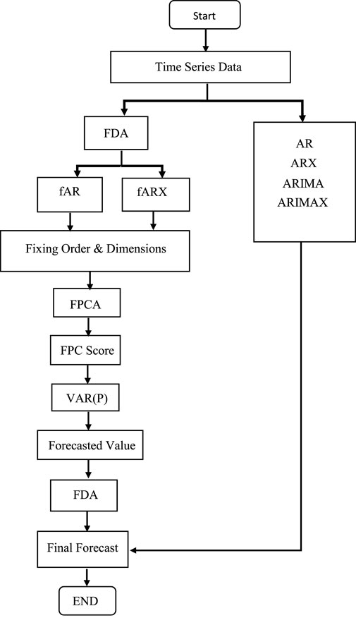
Figure 1. British Electricity Market: architecture of the proposed functional data analysis approach.

2.5 Quality measures

This study has computed numerous quality indicators to compare the models. We convert the anticipated curves into half-hourly electricity pricing data to facilitate comparison. Three average accuracy measures are used to evaluate prediction accuracy and efficiency: 1) mean absolute percentage error (MAPE), 2) mean absolute error (MAE), and 3) root mean square error (RMSE), as well as the Diebold–Mariano equal forecasts statistical test (Quispe et al., 2024; Qureshi et al., 2024).

2.5.1 Mean absolute error

The MAE is derived by averaging the absolute difference between the prediction and the actual value while ensuring that the negative value does not cancel out the positive values. It can be stated thus:

$\text{MAE}=\text{mean}(|{\mathcal{Y}}_{i,k}-{\widehat{\mathcal{Y}}}_{i,k}|)$

where ${\mathcal{Y}}_{i,k}$ is the observed data and ${\widehat{\mathcal{Y}}}_{i,k}$ is the predicted day-ahead electricity price for $i^{th}(i=\mathrm{1,2},\dots ,365)$ day and $k^{\text{th\hspace{0.17em}}}(k=\mathrm{1,2},\dots ,48)$ price period.

2.5.2 Mean absolute percentage error

To compute the MAPE, divide the average absolute error for each period by the observed values and multiply by 100. The MAPE effectively measures accuracy when a prediction variable is large (Box, 2013). It is a relative measure of forecast error that highlights the degree of difference between the predicted and actual values. The mathematical expression for the MAPE is

$\begin{array}{cc}\hfill \text{MAPE}\hfill & =\text{mean}(|\frac{{\mathcal{Y}}_{i,k}-{\widehat{\mathcal{Y}}}_{i,k}}{{\mathcal{Y}}_{i,k}}|)\times 100\hfill \end{array}$

2.5.3 Root mean square error

The RMSE grows as the scale of the dependent variable grows. It compares forecasts from many models for the same dataset. The RMSE is the square root of the squared difference on average between the anticipated and actual values. The mathematical definition is:

$\begin{array}{cc}\hfill RMSE\hfill & \hfill =\sqrt{\text{mean}{({\mathcal{Y}}_{i,k}-{\widehat{\mathcal{Y}}}_{i,k})}^2}\hfill \end{array}$

2.5.4 The Diebold-Mariano test

The Diebold–Mariano (DM) test (McKenzie, 2011) is employed to evaluate the accuracy of the proposed functional time series forecasting models. This statistical test is commonly used in time series analysis to compare the accuracy of two forecasting models. It evaluates whether the errors generated by one model statistically differ from the errors of another (Carbo-Bustinza et al., 2023). To perform the DM test, the forecast errors of each model are calculated using a loss function. These errors are the differences between the observed values $(v_m)$ and the forecast values $({\widehat{v}}_m)$. The test statistic is then calculated by comparing the mean squared errors of the two models. Suppose the test statistic is greater than a certain threshold and the p-value is lower than a pre-determined significance level (e.g., ${\alpha }_{=}0.05$); in that case, we conclude that the forecasts from one model are statistically significantly better than the other.

The null and alternative hypotheses of the DM test are

$H_0$—there is no difference in forecast accuracy between the two models $(H_0:\bar{d}=0)$.

$H_a$—the two models differ in forecast accuracy $(H_a:\bar{d}\ne 0)$.

Therefore, the null hypothesis implies no statistically significant difference in forecast accuracy between the models, while the alternative hypothesis suggests that a significant difference exists.

3 Case study and results

The liberalization of the United Kingdom’s electricity industry can be attributed to the regulatory and structural changes implemented in the late 1980s. These reforms sought to eliminate the state-owned monopoly and establish a competitive wholesale energy market. Recognizing that transmission and distribution are natural monopolies, the main focus of the reforms was the deregulation of the generation and supply sectors. Consequently, in 1990 the UK electricity market underwent reorganization, establishing the England and Wales power pool and dividing the government monopoly into three entities: National Power, Powergen, and Nuclear Energy.

The power pool served as a trading platform for half-hourly transactions. However, market power in the generation industry became a significant concern due to National Power and Powergen holding respective market shares of 50% and 30%. Meanwhile, Nuclear Electric, responsible for supplying the base load of nuclear power, essentially acted as a price taker. Market manipulation by these two corporations led to reduced competition, resulting in the average price remaining approximately 24 per megawatt-hour between 1994 and 1996 (Karakatsani and Bunn, 2008).

A fully liberalized bilateral contracting system replaced the England and Wales power pool with the introduction of New Energy Trading Arrangements (NETA) in 2001 (becoming the British Electricity Trading Transmission Arrangements—BETTA—in 2005). This transition established a more stable market share for electricity companies in the generation and retail sectors. Additionally, the reforms resulted in the creation of three distinct power exchanges: the United Kingdom Power Exchange (UKPX), the UK Automated Power Exchange (APX UK), and the International Exchange (IE, formerly known as the International Petroleum Exchange—IPE). Subsequently, the amalgamation of APX and UKPX into APX Group in 2004, followed by the inclusion of Scotland in the UK power market in 2005, further enhanced market dynamics. This highly competitive and well-developed market exhibits a robust correlation between market price and market fundamentals (Lisi and Pelagatti, 2018).

3.1 Data description and forecasting results

This study aims to accurately and efficiently forecast half-hourly electricity pricing data from APX from January 2018 to December 2022. To achieve this objective, we implemented an FDA to model and forecast the electricity price-time series in the APX. To understand the complex characteristics of electricity price dynamics over time, these characteristics are expected to include missing values, a nonlinear long-run secular trend, pronounced seasonality, high volatility, non-normality, and non-stationarity. A non-stationary process can be defined as one in which statistical features such as mean, variance, and autocorrelation vary with time. This indicates that the data lacks a steady mean or variance, making it difficult to examine using typical statistical approaches that presume stationarity. Thus, the key characteristics of non-stationary data are: a) trends: non-stationary data may show long-term trends in which values grow or decrease with time; b) seasonality: refers to recurrent patterns or cycles that occur at regular periods, such as seasonal influences in sales statistics; c) changing variability: the variability of the data may alter with time, resulting in periods of volatility followed by stability. For instance, Figure 2A shows the half-hourly electricity price time series with a red-line linear and blue-line nonlinear trend component. Figure 2B shows a boxplot for the half-hourly over 6 years, indicating high variations among the 24 hours (48 half hours). Figure 2C shows the autocorrelation plot of the original electricity prices at 336 lags, and Figure 2D shows the partial autocorrelation plot of original electricity prices at 336. These figures clearly illustrate a discernible long-term trend, as well as annual and weak seasonality. Furthermore, non-normality and non-stationarity are also evident from these visual representations.

Figure 2

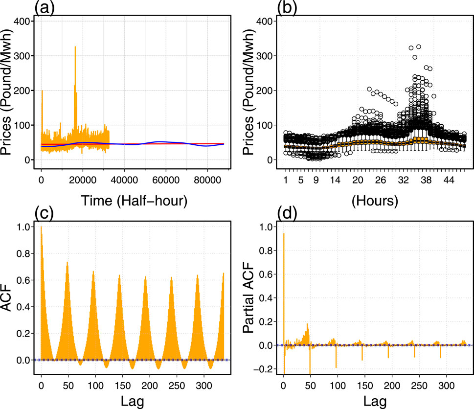
Figure 2. Characterization of British electricity power prices (2018–2022): time diagrams (a) visualize time fluctuations using long-term linear (blue) and non-linear (red) trend components; (b) half-hour sequence diagrams; (c) autocorrelation function diagrams analyze the correlation of price fluctuations during various past delays; (d) partial autocorrelation function diagrams investigate the relationship between price changes after accounting for the effects of previous delays.

On the other hand, Table 1 summarizes the characteristics of the data before and after data transformations, such as taking the natural logarithm (addressing variance and standard deviation stabilization). For instance, for the electric power time series before and after data transformations, the minimum values: are 2.20 and 0.79, first quartile (37.28 and 3.62); median (43.96 and 3.78); mean (45.51 and 3.79); mode (37.81 and 3.63); third quartile (51.28 and 3.94); standard deviation (12.45 and 0.25); coefficient of variation (27.36 and 6.56); maximum (326.09 and 5.79). It is confirmed from this analysis that the log transformation attained normality in the data since the mean, median, and mode are approximately the same. However, the standard deviation is also much lower than the original series. To this end, further analysis proceeds with the log-transformed electric power price series for modeling and forecasting purposes. Thus, for modeling and forecasting, the log-transformed data are divided into two parts:

• validation data: from $1^{st}$ January 2018 to $31^{st}$ December 2021 (70,128 observations, covering i = 1461 days)

• testing data: from $1^{st}$ January 2022 until $1^{st}$ December 2022 (17,520 data points (hours), with i = 365 (days).

Table 1

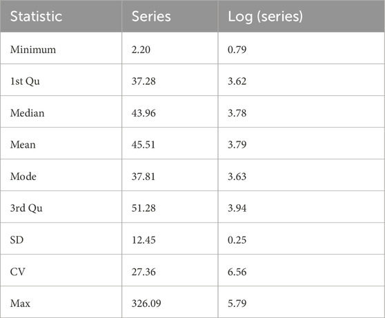
Table 1. Summary statistics of British Electricity Market 2018–2022.

The models were estimated using an extension window approach derived from an annual 1-day out-of-sample forecast. As indicated in Figure 3, the discrete half-hourly electricity price is from $1^{st}$ January 2018 to $31^{st}$ December 2022. The Fourier base function transforms the discrete electricity power price data into a functional form (Figure 4). The mean curve can be represented with a solid black curve.

Figure 3

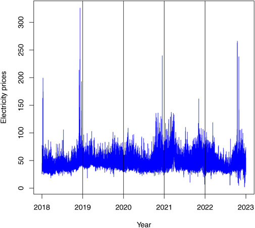
Figure 3. British Electricity Market: figure represents the discrete half-hourly data of 5 years.

Figure 4

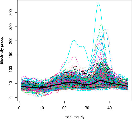
Figure 4. British Electricity Market: functional daily curves for British electricity prices; ${\mathcal{Y}}_i(\tau )i=1,\dots ,1826$, where ${\mathcal{Y}}_i(\tau )$ are the natural log-transformed functional data points of half-hourly electric power pricing using 22 Fourier basis functions. The solid black curve is the mean curve.

Figure 5 illustrates that the functional representation of electricity prices exhibits lower values during weekends than weekdays, indicating less electricity use over weekends. Figure 6 shows the first five FPCs, which account for a large number of data variations. Figure 7 shows the proportion of variation explained by each FPC. The graphic shows that the first PC accounts for about 60% of all data volatility. Accordingly, the second, third, fourth, and fifth FPCs account for 13%, 8%, 6%, and 5% of total variation.

Figure 5

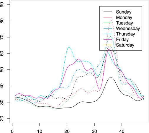
Figure 5. British Electricity Market: graphic functional description of a single week of electricity prices.

Figure 6

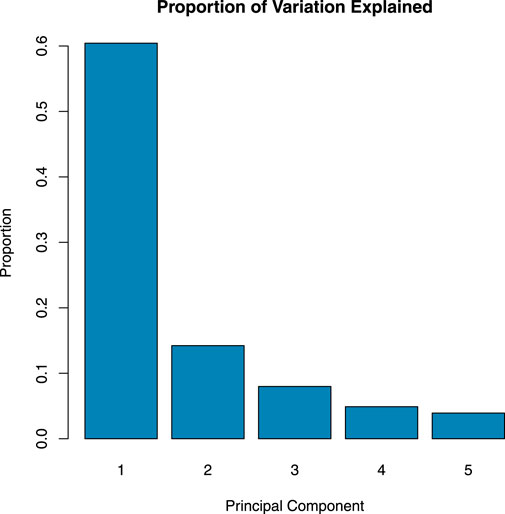
Figure 6. British Electricity Market: five principal components proportion of variation explained by each FPC.

Figure 7

Figure 7. British Electricity Market: first five FPCs.

The day-ahead forecasting accuracy of the models is measured using the MAE, MAPE, and RMSE. For instance, Table 2 summarizes the models’ overall accuracy, showing that the functional models outperform the classical time series models (AR, AR$\mathbb{X}$, ARIMA, and ARIMA$\mathbb{X}$ models). Within the functional models, $\mathbb{F}$AR$\mathbb{X}$)$(\mathcal{P})$ demonstrates superior forecasting performance compared to $\mathbb{F}$AR$(\mathcal{P})$. For instance, $\mathbb{F}$AR$\mathbb{X}$)$(\mathcal{P})$ achieves the lowest mean error—MAPE = 5.95, MAE = 4.17, and RMSE = 12.94—comparatively lower than the $\mathbb{F}$AR$(\mathcal{P})$ model. On the other hand, the functional models ($\mathbb{F}$AR$(\mathcal{P})$ and $\mathbb{F}$AR$\mathbb{X}$)$(\mathcal{P})$) compared to the classical time series models (AR, AR$\mathbb{X}$, ARIMA, and ARIMA$\mathbb{X}$) obtain highly accurate forecasting mean errors. For example, $\mathbb{F}$AR$\mathbb{X}$)$(\mathcal{P})$ improves the forecasting mean errors ranging from 32.96%–84.41%, 36.22%–225.93%, and 17.81%–69.40%, for the MAPE, MAE, and RMSE, respectively. Therefore, the relatively least accurate mean error values across the board demonstrate the usefulness of the $\mathbb{F}$AR$\mathbb{X}$)$(\mathcal{P})$ forecasting model.

Table 2

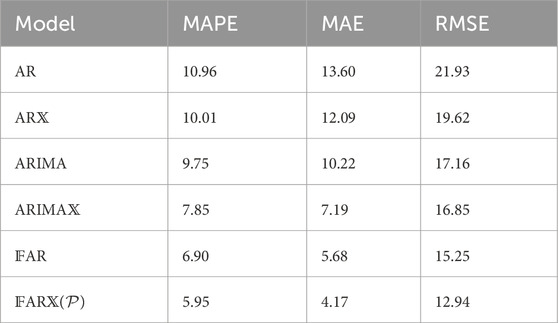
Table 2. British Electricity Market: out-of-sample forecasting error evaluation of functional models and traditional time series models considered.

On the other hand, a graphical comparison (Figure 8) shows the original and predicted values for each of the forecasting models that were taken into account in Table 2. The figure demonstrates how well the forecast from the proposed functional model ($\mathbb{F}$AR$\mathbb{X}$($\mathcal{P}$) matches the actual pricing. However, the $\mathbb{F}$AR$\mathbb{X}$ and $\mathbb{F}$AR show competitive results. The classic AR model shows the worst forecasting results among all models considered. Therefore, we can determine that the $\mathbb{F}$AR$\mathbb{X}$($\mathcal{P}$ model outperformed the rest of the models.

Figure 8

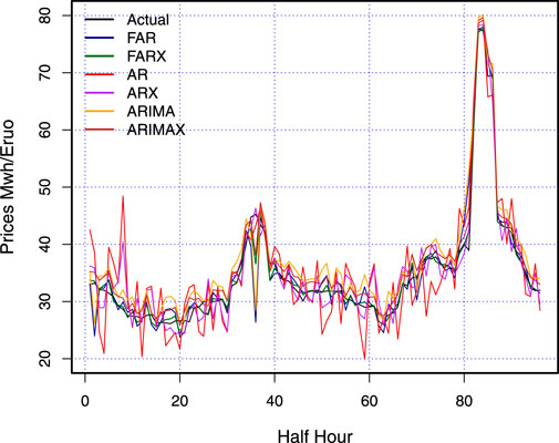
Figure 8. British Electricity Market: out-of-sample forecasting error evaluation of the functional models and considered traditional time series models.

After calculating the accuracy measures (MAPE, MAE, and RMSE), the Diebold–Mariano (DM) test was used to statistically assess the superiority of the proposed functional time series models (see Table 3 for the DM statistic p-values). The outcome of this table revealed that the proposed functional time series model ($\mathbb{F}$AR$\mathbb{X}$)$(\mathcal{P})$) achieved statistically superior performance across all models; the $\mathbb{F}$AR$(\mathcal{P})$ model showed the second-best results. These findings confirm $\mathbb{F}$AR$\mathbb{X}$)$(\mathcal{P})$ as the most reliable model for day-ahead electricity price forecasting within the scope of this study.

Table 3

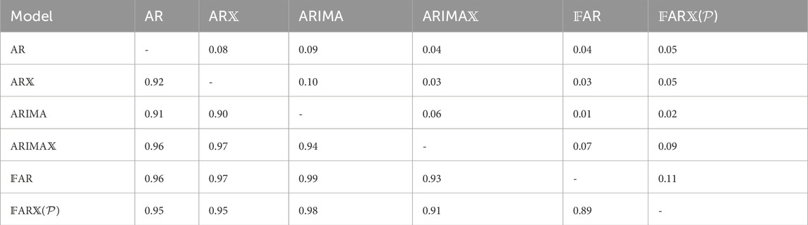
Table 3. British Electricity Market: Diebold–Mariano results (p-value) for all forecasting models.

Table 4 displays the weekly forecasting errors for the models under investigation. Monday, Wednesday, Saturday, and Sunday are typically associated with larger weekly errors than Tuesday, Thursday and Friday. Among the models, $\mathbb{F}$AR$\mathbb{X}$($\mathcal{P}$) achieves the lowest MAPE value of 3.99 on Thursday—a day with a relatively stable electricity load. Conversely, Sunday exhibits a higher MAPE score of 9.72. Consistent with the previous tables, the functional model with the deterministic component, $\mathbb{F}$AR$\mathbb{X}$($\mathcal{P}$), outperforms the partial functional method, $\mathbb{F}$AR ($\mathcal{P}$). In contrast, the classical univariate time series models (AR, AR$\mathbb{X}$, ARIMA, and ARIMA$\mathbb{X}$) perform relatively poorly compared to the other models considered in this study.

Table 4

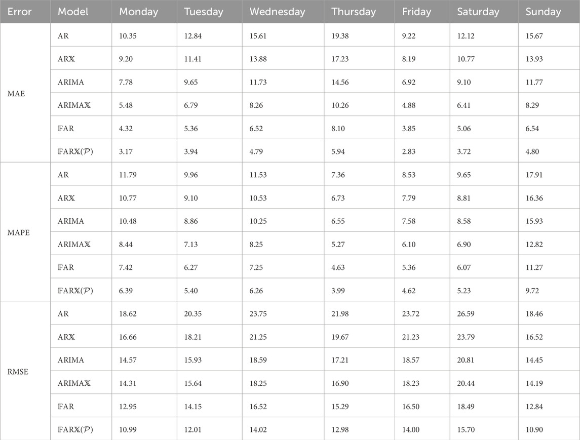
Table 4. British Electricity Market: weekly forecasting accuracy metrics evaluation of functional models and traditional time series models considered.

Table 5 presents the monthly forecasting errors for each model considered in this study. It is evident that December, January, and February exhibit relatively higher errors than other months. This can be attributed to increased electricity demand during these months. Nevertheless, the functional models perform better than the standard traditional time series models. Specifically, the direct functional model $\mathbb{F}$AR$\mathbb{X}$)$(\mathcal{P})$ exhibits lower forecasting errors than the other methods discussed here. The MAPE values for $\mathbb{F}$AR$\mathbb{X}$)$(\mathcal{P})$ range 3.034–6.486, indicating the effectiveness of this model.

Table 5

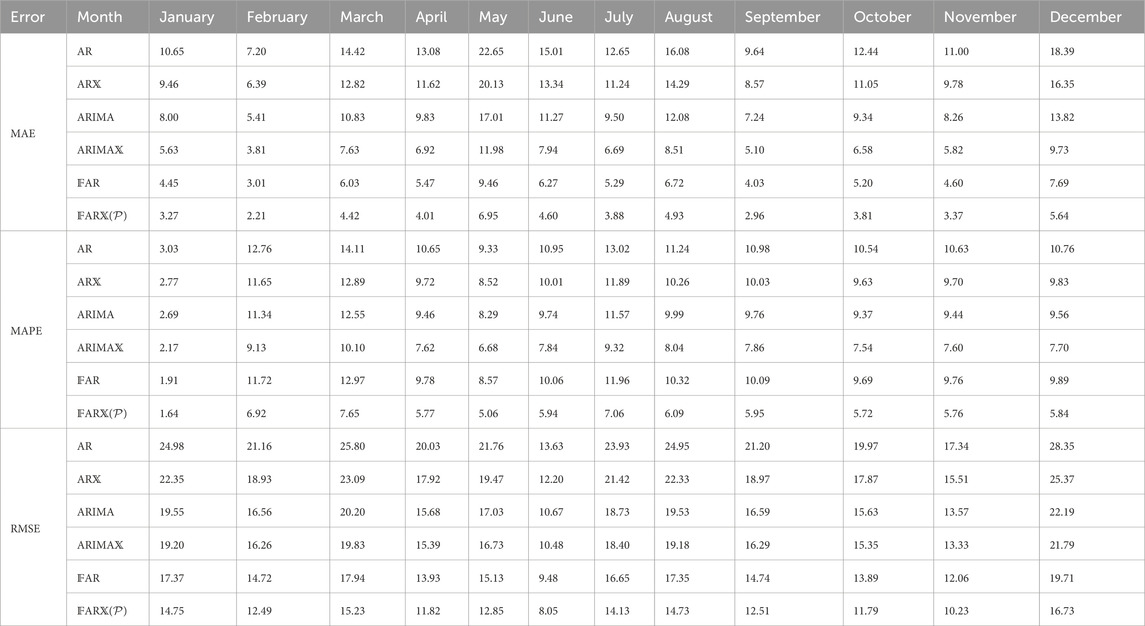
Table 5. British Electricity Market: monthly forecasting accuracy evaluation of functional models and traditional time series models considered.

As is evident from the average accuracy errors (MAE, MAPE, and RMSE) and equal forecasting accuracy statistical test (DM test) and graphical results (line plots), the $\mathbb{F}$AR$\mathbb{X}$)$(\mathcal{P})$ model outperforms its counterpart, the $\mathbb{F}$AR model, and the standard classical time series models (AR, AR$\mathbb{X}$, ARIMA, and ARIMA$\mathbb{X}$). However, the effect of modifying the function models by incorporating the deterministic part was clearly seen, where the exogenous variables are denoted by long trend, yearly periodicity, seasonal periodicity, bank holidays, and electricity demand. Using these exogenous variables, the functional model is modified to $\mathbb{F}$AR$\mathbb{X}$($\mathcal{P}$). The optimal dimension and order are chosen through fFPE. The vector AR model uses a scores vector and then a 1-day forecast of the aforementioned model.

To sum up this section, we can say that the suggested functional forecasting model with exogenous variables has a high degree of accuracy and efficiency for day-ahead for British electricity prices based on the accuracy mean errors (MAE, MAPE, and RMSE) and equal forecast statistical test (the DM test).

4 Discussion

This section compares the best proposed functional ($\mathbb{F}$AR$\mathbb{X}$($\mathcal{P}$)) forecasting model in this study with the proposed best models in the literature. A detailed comparison of this study’s best forecasting functional model with the literature’s best models is listed in Table 6. This confirms that the proposed (Stochastic-AR) best model from Lisi and Pelagatti (2018) has been applied to the database utilized in the current work, and the average accuracy metrics have been calculated. The average accuracy metrics values reported for the proposed (Stochastic-AR) best model of Lisi and Pelagatti (2018) are MAPE = 9.81 (65.01%), MAE = 11.29 (170.61%), and RMSE = 18.12 (40.00%), which are significantly higher than our accuracy mean error values: MAPE = 5.95, MAE = 4.17, and RMSE = 12.94. The proposed (the FAR(P) model) best model in Jan et al. (2022) has been compared to the current research dataset and produced performance metrics comparatively higher than our proposal (the $\mathbb{F}$AR$\mathbb{X}$($\mathcal{P}$) model). For example, the computed forecasting average errors using the proposed (the FAR(P) model) best model in Jan et al. (2022) are 6.50, 5.18, and 14.55—significantly higher than our proposed ($\mathbb{F}$AR$\mathbb{X}$($\mathcal{P}$)) best model forecasting average accuracy errors. Additionally, in Iftikhar et al. (2023c), the proposed (the best model ⁴${\text{RSD}}_3^4$) was used in our dataset obtained mean accuracy metrics also comparatively greater than the $\mathbb{F}$AR$\mathbb{X}$($\mathcal{P}$) model at 4.46%, 20.81%, and 10.02% for the MAPE, MAE, and RMSE, respectively. Furthermore, the developed best model (Ensemble) of Bibi et al. (2021) was used in the current research database and the average metric errors computed, such as MAPE, MAE, and RMSE—comparatively higher (5.30%, 23.20%, and 11.10%) than our best functional model. In Shah et al. (2022a), the best forecasting model (^NP${\text{VAR}}_E$) was applied to our database and the average mean errors computed. However, in comparison, the computed mean errors in the ${\text{NPVAR}}_E$ forecasting model were 10.68%, 27.52%, and 11.18% for the MAPE, MAE, and RMSE, respectively—higher than our best functional model. In summary, it is evident that the best functional model of this work achieved higher accuracy than the best models found in the literature.

Table 6

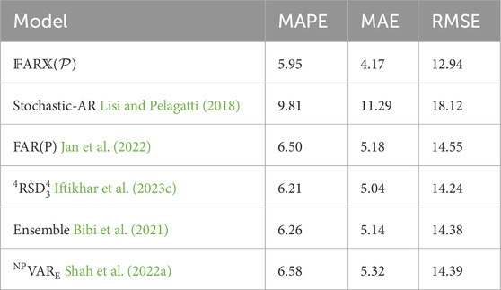
Table 6. British Electricity Market (pound/MWh): comparison of one-day-ahead average accuracy metrics between proposed functional best models and literature best models.

Table 7

Table 7. Table of nomenclature.

The proposed functional time series model used in this study has proven to be very accurate and effective in predicting the next-day power price in the British electricity market. These precise forecasts can help sellers (buyers and suppliers) optimize their bid planning, maximize revenue, and better use the resources required to generate electricity. Offering a stable and cost-effective energy system benefits end users. Furthermore, the accurate projection and understanding of energy prices in developing countries can help traders make more effective commercial and trade plans and better asset allocations. Finally, sellers (buyers and suppliers) can create more robust trading strategies based on the proposed $\mathbb{F}$AR$\mathbb{X}$($\mathcal{P}$) model and choose models with the most remarkable risk reward ration.

The statistical computing language programming environment R-studio implements analysis models. In comparison, all computations were performed with Intel(R) Core(TM) i7-6600 @ 2.80 GHz CPU. R uses GAM, tsDyn, and forecast libraries to model and predict standard time series forecast models. We wrote our own source code to model and forecast $\mathbb{F}$AR$\mathbb{X}$ and $\mathbb{F}$AR$\mathbb{X}$($\mathcal{P}$) models, which also use R’s fda library. The documentation of the packages provides detailed information on the algorithms used in the estimation.

5 Conclusion

Forecasting electricity prices in a deregulated power market is complex and crucial. The price time series of electric power exhibits features such as high frequency, long-term trends, multiple seasonal patterns, spikes or jumps, and the effects of bank holidays. Addressing these features is essential for accurate price forecasting. This study has focused on the problem of day-ahead electricity price forecasting using functional data analysis. The electricity prices were modeled and forecast through two functional models, employing four classical time series models (AR, AR$\mathbb{X}$, ARIMA, and ARIMA$\mathbb{X}$) for this purpose. The price series was transformed into a functional form, and $\mathbb{F}$AR$(\mathcal{P})$ was utilized for modeling and forecasting. The functional model was further modified by introducing some essential exogenous information (specific features): $\mathbb{F}$AR$\mathbb{X}$($\mathcal{P}$). Meanwhile, the AR, AR$\mathbb{X}$, ARIMA, and ARIMA$\mathbb{X}$ models employed conventional time series models for modeling and forecasting electricity prices. In comparison to the benchmark models (AR, AR$\mathbb{X}$, ARIMA, ARIMA$\mathbb{X}$, and the proposed $\mathbb{F}$AR model), the $\mathbb{F}$AR$\mathbb{X}$ model reduces the day-ahead forecasting average MAPE by a range of 5.02%–45.77%, 4.07%–40.63%, 3.80%–38.99%, 1.90%–24.22%, and 0.95%–13.78%; MAE by a range of 9.43%–69.32%, 5.17%–65.48%, 6.04%–59.16%, 3.02%–42.01%, and 1.51%–26.59%; RMSE by a range of 8.98%–40.97%, 6.68%–34.03%, 4.22%–24.58%, 3.91%–23.20%, and 2.30%–15.11%. Furthermore, compared with the literature’s proposed best models, the $\mathbb{F}$AR$\mathbb{X}$ model produces a significantly higher accuracy and efficient day-ahead forecast based on forecasting error indicators and an equal forecast statistical test. Compared with the best models proposed in the literature, the $\mathbb{F}$AR$\mathbb{X}$ model demonstrates significantly higher accuracy and efficiency in day-ahead forecasting, as evidenced by forecasting error indicators and an equal forecast statistical test.

This study focuses entirely on the British electricity market. The idea should include additional electrical markets, such as the European, American, and Chinese markets. Other energy market factors are electricity demand, production, consumption, curves, natural gas pricing, wind speed, and crude oil prices. This will enable a more in-depth assessment of the upgraded functional model’s performance. There are various approaches to broaden the field of future study. Other functional factors, such as temperature, consumer load, fuel, carbon dioxide emission costs, average solar radiation, and wind speed, can be included in the model to improve electricity price forecasting accuracy.

Data availability statement

Publicly available datasets were analyzed in this study; the data can be found at: https://www.kaggle.com/datasets/thedevastator/gb-electrical-grid-half-hourly-data-2008-present.

Author contributions

FJ: conceptualization, data curation, formal analysis, investigation, methodology, resources, software, validation, visualization, writing–original draft, and writing–review and editing. HI: conceptualization, formal analysis, funding acquisition, methodology, project administration, resources, software, supervision, visualization, writing–original draft, and writing–review and editing. MT: data curation, formal analysis, investigation, resources, and writing–review and editing. MK: funding acquisition, investigation, project administration, supervision, and writing–review and editing.

Funding

The authors declare that no financial support was received for the research, authorship, and/or publication of this article.

Conflict of interest

The authors declare that the research was conducted in the absence of any commercial or financial relationships that could be construed as a potential conflict of interest.

Publisher’s note

All claims expressed in this article are solely those of the authors and do not necessarily represent those of their affiliated organizations, or those of the publisher, the editors, and the reviewers. Any product that may be evaluated in this article, or claim that may be made by its manufacturer, is not guaranteed or endorsed by the publisher.

References

Aue, A., Norinho, D. D., and Hörmann, S. (2015). On the prediction of stationary functional time series. J. Am. Stat. Assoc. 110, 378–392. doi:10.1080/01621459.2014.909317

CrossRef Full Text | Google Scholar

Baruah, R. D., and Organero, M. M. (2023). “Integrating explicit contexts with recurrent neural networks for improving prognostic models,” in 2023 IEEE aerospace conference Germany, (IEEE), 1–8.

CrossRef Full Text | Google Scholar

Bibi, N., Shah, I., Alsubie, A., Ali, S., and Lone, S. A. (2021). Electricity spot prices forecasting based on ensemble learning. IEEE Access 9, 150984–150992. doi:10.1109/access.2021.3126545

CrossRef Full Text | Google Scholar

Bosq, D. (2000). Linear processes in function spaces: theory and applications. Germany, Springer Science and Business Media. 149.

Google Scholar

Bosq, D., and Blanke, D. (2008). Inference and prediction in large dimensions. John Wiley and Sons.

Google Scholar

Box, G. (2013). “Box and jenkins: time series analysis, forecasting and control,” in A very British affair: six britons and the development of time series analysis during the 20th century Germany, (Springer), 161–215.

Google Scholar

Carbo-Bustinza, N., Iftikhar, H., Belmonte, M., Cabello-Torres, R. J., De La Cruz, A. R. H., and López-Gonzales, J. L. (2023). Short-term forecasting of ozone concentration in metropolitan lima using hybrid combinations of time series models. Appl. Sci. 13, 10514. doi:10.3390/app131810514

CrossRef Full Text | Google Scholar

Chan, S.-C., Tsui, K. M., Wu, H., Hou, Y., Wu, Y.-C., and Wu, F. F. (2012). Load/price forecasting and managing demand response for smart grids: methodologies and challenges. IEEE signal Process. Mag. 29, 68–85. doi:10.1109/msp.2012.2186531

CrossRef Full Text | Google Scholar

Chaouch, M. (2013). Clustering-based improvement of nonparametric functional time series forecasting: application to intra-day household-level load curves. IEEE Trans. Smart Grid 5, 411–419. doi:10.1109/tsg.2013.2277171

CrossRef Full Text | Google Scholar

Chen, Y., Chua, W. S., and Koch, T. (2018). Forecasting day-ahead high-resolution natural-gas demand and supply in Germany. Appl. energy 228, 1091–1110. doi:10.1016/j.apenergy.2018.06.137

CrossRef Full Text | Google Scholar

Chen, Y., and Li, B. (2017). An adaptive functional autoregressive forecast model to predict electricity price curves. J. Bus. and Econ. Statistics 35, 371–388. doi:10.1080/07350015.2015.1092976

CrossRef Full Text | Google Scholar

Coelho, C., Costa, M. F. P., and Ferrás, L. L. (2024). Enhancing continuous time series modelling with a latent ode-lstm approach. Appl. Math. Comput. 475, 128727. doi:10.1016/j.amc.2024.128727

CrossRef Full Text | Google Scholar

Dudek, G. (2015). “Short-term load forecasting using random forests,” in Intelligent systems’ 2014: proceedings of the 7th IEEE international conference intelligent systems IS’2014, Warsaw, Poland, September 24-26, 2014, , volume 2: tools, architectures, systems, applications (Springer), 821–828.

Google Scholar

Fargalla, M. A. M., Yan, W., Deng, J., Wu, T., Kiyingi, W., Li, G., et al. (2024). Timenet: time2vec attention-based cnn-bigru neural network for predicting production in shale and sandstone gas reservoirs. Energy 290, 130184. doi:10.1016/j.energy.2023.130184

CrossRef Full Text | Google Scholar

Gers, F. A., Eck, D., and Schmidhuber, J. (2001). “Applying lstm to time series predictable through time-window approaches,” in International conference on artificial neural networks USA, 9 to September 12, 2025, (Springer), 669–676.

Google Scholar

Gonzales, S. M., Iftikhar, H., and López-Gonzales, J. L. (2024). Analysis and forecasting of electricity prices using an improved time series ensemble approach: an application to the peruvian electricity market. AIMS Math. 9, 21952–21971. doi:10.3934/math.20241067

CrossRef Full Text | Google Scholar

Hippert, H. S., Pedreira, C. E., and Souza, R. C. (2001). Neural networks for short-term load forecasting: a review and evaluation. IEEE Trans. power Syst. 16, 44–55. doi:10.1109/59.910780

CrossRef Full Text | Google Scholar

Horváth, L., and Kokoszka, P. (2012). Inference for functional data with applications, Springer Science and Business Media. 200.

Google Scholar

Iftikhar, H., Bibi, N., Canas Rodrigues, P., and López-Gonzales, J. L. (2023a). Multiple novel decomposition techniques for time series forecasting: application to monthly forecasting of electricity consumption in Pakistan. Energies 16, 2579. doi:10.3390/en16062579

CrossRef Full Text | Google Scholar

Iftikhar, H., Turpo-Chaparro, J. E., Canas Rodrigues, P., and López-Gonzales, J. L. (2023b). Day-ahead electricity demand forecasting using a novel decomposition combination method. Energies 16, 6675. doi:10.3390/en16186675

CrossRef Full Text | Google Scholar

Iftikhar, H., Turpo-Chaparro, J. E., Canas Rodrigues, P., and López-Gonzales, J. L. (2023c). Forecasting day-ahead electricity prices for the Italian electricity market using a new decomposition—combination technique. Energies 16, 6669. doi:10.3390/en16186669

CrossRef Full Text | Google Scholar

Inglada-Pérez, L., and Gil, S. G. y. (2024). A study on the nature of complexity in the Spanish electricity market using a comprehensive methodological framework. Mathematics 12, 893. doi:10.3390/math12060893

CrossRef Full Text | Google Scholar

Jan, F., Shah, I., and Ali, S. (2022). Short-term electricity prices forecasting using functional time series analysis. Energies 15, 3423. doi:10.3390/en15093423

CrossRef Full Text | Google Scholar

Karakatsani, N. V., and Bunn, D. W. (2008). Forecasting electricity prices: the impact of fundamentals and time-varying coefficients. Int. J. Forecast. 24, 764–785. doi:10.1016/j.ijforecast.2008.09.008

CrossRef Full Text | Google Scholar

Karim, F., Majumdar, S., Darabi, H., and Harford, S. (2019). Multivariate lstm-fcns for time series classification. Neural Netw. 116, 237–245. doi:10.1016/j.neunet.2019.04.014

PubMed Abstract | CrossRef Full Text | Google Scholar

Kokoszka, P., and Reimherr, M. (2013). Determining the order of the functional autoregressive model. J. Time Ser. Analysis 34, 116–129. doi:10.1111/j.1467-9892.2012.00816.x

CrossRef Full Text | Google Scholar

Lago, J., Marcjasz, G., De Schutter, B., and Weron, R. (2021). Forecasting day-ahead electricity prices: a review of state-of-the-art algorithms, best practices and an open-access benchmark. Appl. Energy 293, 116983. doi:10.1016/j.apenergy.2021.116983

CrossRef Full Text | Google Scholar

Li, J., Deng, D., Zhao, J., Cai, D., Hu, W., Zhang, M., et al. (2020). A novel hybrid short-term load forecasting method of smart grid using mlr and lstm neural network. IEEE Trans. Industrial Inf. 17, 2443–2452. doi:10.1109/tii.2020.3000184

CrossRef Full Text | Google Scholar

Lisi, F., and Pelagatti, M. M. (2018). Component estimation for electricity market data: deterministic or stochastic? Energy Econ. 74, 13–37. doi:10.1016/j.eneco.2018.05.027

CrossRef Full Text | Google Scholar

Lisi, F., and Shah, I. (2020). Forecasting next-day electricity demand and prices based on functional models. Energy Syst. 11, 947–979. doi:10.1007/s12667-019-00356-w

CrossRef Full Text | Google Scholar

Liu, B., Fu, C., Bielefield, A., and Liu, Y. Q. (2017). Forecasting of Chinese primary energy consumption in 2021 with gru artificial neural network. Energies 10, 1453. doi:10.3390/en10101453

CrossRef Full Text | Google Scholar

McKenzie, J. (2011). Mean absolute percentage error and bias in economic forecasting. Econ. Lett. 113, 259–262. doi:10.1016/j.econlet.2011.08.010

CrossRef Full Text | Google Scholar

Paparoditis, E., and Sapatinas, T. (2013). Short-term load forecasting: the similar shape functional time-series predictor. IEEE Trans. power Syst. 28, 3818–3825. doi:10.1109/tpwrs.2013.2272326

CrossRef Full Text | Google Scholar

Pinhão, M., Fonseca, M., and Covas, R. (2022). Electricity spot price forecast by modelling supply and demand curve. Mathematics 10, 2012. doi:10.3390/math10122012

CrossRef Full Text | Google Scholar

Quispe, F., Salcedo, E., Iftikhar, H., Zafar, A., Khan, M., Turpo-Chaparro, J. E., et al. (2024). Multi-step ahead ozone level forecasting using a component-based technique: a case study in lima, Peru. AIMS Environ. Sci. 11, 401–425. doi:10.3934/environsci.2024020

CrossRef Full Text | Google Scholar

Qureshi, M., Iftikhar, H., Rodrigues, P. C., Rehman, M. Z., and Salar, S. A. (2024). Statistical modeling to improve time series forecasting using machine learning, time series, and hybrid models: a case study of bitcoin price forecasting. Mathematics 12, 3666. doi:10.3390/math12233666

CrossRef Full Text | Google Scholar

Rajabi, R., and Estebsari, A. (2019). “Deep learning based forecasting of individual residential loads using recurrence plots,” in 2019 IEEE milan PowerTech (IEEE), 1–5.

CrossRef Full Text | Google Scholar

Shah, I., Iftikhar, H., and Ali, S. (2022a). Modeling and forecasting electricity demand and prices: a comparison of alternative approaches. J. Math. 2022, 3581037. doi:10.1155/2022/3581037

CrossRef Full Text | Google Scholar

Shah, I., Iftikhar, H., Ali, S., and Wang, D. (2019). Short-term electricity demand forecasting using components estimation technique. Energies 12, 2532. doi:10.3390/en12132532

CrossRef Full Text | Google Scholar

Shah, I., Jan, F., and Ali, S. (2022b). Functional data approach for short-term electricity demand forecasting. Math. problems Eng. 2022, 1–14. doi:10.1155/2022/6709779

CrossRef Full Text | Google Scholar

Taheri, S., Talebjedi, B., and Laukkanen, T. (2021). Electricity demand time series forecasting based on empirical mode decomposition and long short-term memory. Energy Eng. J. Assoc. Energy Eng. 118, 1577–1594. doi:10.32604/ee.2021.017795

CrossRef Full Text | Google Scholar

Talebjedi, B., Laukkanen, T., and Holmberg, H. (2024). Integration of thermal energy storage for sustainable energy hubs in the forest industry: a comprehensive analysis of cost, thermodynamic efficiency, and availability. Heliyon 10, e36519. doi:10.1016/j.heliyon.2024.e36519

PubMed Abstract | CrossRef Full Text | Google Scholar

Ugurlu, U., Oksuz, I., and Tas, O. (2018). Electricity price forecasting using recurrent neural networks. Energies 11, 1255. doi:10.3390/en11051255

CrossRef Full Text | Google Scholar