Solar-heat-assisted hydrogen production using solid oxide electrolysis cells in Japan

Japan and other industrialized countries rely on the import of green hydrogen (H₂) as they lack the resources to meet their own demand. In contrast, countries such as Australia have the potential to produce hydrogen and its derivatives using wind and solar energy. Solar energy can be harnessed to produce electricity using photovoltaic systems or to generate thermal energy by concentrating solar irradiation. Thus, thermal and electrical energy can be used in a solid oxide electrolysis process for low-cost hydrogen production. The operation of a solid oxide electrolysis cell (SOEC) stack integrated with solar energy is experimentally investigated and further analyzed using a validated simulation model. Furthermore, a techno-economic assessment is conducted to estimate the hydrogen production costs, including the expenses associated with liquefaction and transportation from Australia to Japan. High conversion efficiencies and low-cost SOECs are projected to result in production costs below 4 USD/kg.

1 Introduction

In Japan, Kawasaki Heavy Industries, Ltd., is developing a hydrogen (H₂) production technology that utilizes low-quality coal with carbon capture and storage (CCS) in Australia. The company plans to export the hydrogen to Japan in liquefied form using hydrogen carrier ships. According to Kimura et al. (ERIA, 2020), the cost of H₂ in 2030 was estimated in 2012 to be 4.13 US$/kg (1 US$ (USD) = 80 yen; H₂ gas density is 0.0898 kg/Nm³). The cost analysis for the liquefied hydrogen (LH₂) supply chain consisted of H₂ production, gas purification via pressure swing adsorption, liquefaction, terminal loading, and LH₂ cargo ship transport from Australia to Japan. The present cost of LH₂ may have increased due to the recent global inflation. This technology is relies on the use of fossil fuel and therefore requires the implementation of CCS.

Recently, Japan—like many other industrialized countries—has been experiencing a high demand for energy and green hydrogen. Water electrolysis is considered one of the most important technologies for green hydrogen production (IRENA, 2024). Renewable energy sources such as wind and solar energy can be used through wind turbines and photovoltaic systems, respectively, to generate electricity. However, battery storage remains cost-intensive, and electricity is one of the main cost drivers in water electrolysis. Conventional low-temperature polymer electrolyte membrane (PEM) and alkaline electrolyzers operate at efficiencies of only 70%–80%, while a solid oxide electrolysis cell (SOEC), operating at 600°C–800°C, can achieve an efficiency of 90% or higher when utilizing steam (20% more efficiency). Our previous study showed that the H₂ production cost of an SOEC electrolyzer using thermal energy for steam production will be lower than that of a PEM electrolyzer, based on future cost projections for 2040 at 4,000 full-load hours—or even earlier with increased operating full-load hours (Roeder et al., 2024). Hence, using thermal energy instead of electrical energy to reduce the total electrical energy demand in SOECs is a promising approach due to the higher efficiency of SOECs, which operate at a lower voltage of approximately 1.29 V compared to conventional water electrolysis systems. The steam required for SOEC operation can be generated using concentrated solar power (sunlight); this method can achieve lower costs than electric-based steam generation, especially at night, because of the reduced cost of thermal energy storage.

One of the first studies to couple concentrated solar energy with an SOEC used concentrated light directly onto the electrolysis cell (Arashi et al., 1991). Since then, different concepts have been developed. Most studies focus on low-temperature heat integration as it accounts for the majority of the thermal energy demand (Alzahrani and Dincer, 2016; Monnerie et al., 2017; Mohammadi and Mehrpooya, 2019; Puig-Samper et al., 2022; Ma and Martinek, 2024; Martins et al., 2024). The integration of high-temperature heat can result in an increase in solar-to-fuel efficiency (Lin and Haussener, 2017). Therefore, different receiver concepts have been developed to achieve steam temperatures above 600°C (Houaijia et al., 2014; Kadohiro et al., 2023; Kadohiro et al., 2024; Lin et al., 2022; Schiller et al., 2019), with newer designs reaching temperatures above 800°C for both steam and air (Kadohiro et al., 2025). However, the hydrogen production costs of the previous studies have been estimated to be between 8.61 and 14.89 USD/kg considering an exchange rate of 1 USD = 0.9 € and the chemical engineering plant cost index (CEPCI) to convert the costs to 2023-equivalent costs (Lin and Haussener, 2017; Mastropasqua et al., 2020). Considering the current and planned SOEC costs, degradation rate, and changing operation conditions, large concentrated solar thermal systems have the potential to be cost-competitive with conventional hydrogen production with CCS. For the state-of-the-art electrolysis costs, various reports expect a similar cost development, and the total investment cost of electrolysis is considered to have a high impact on the final production costs. The total cost of the electrolysis system comprises the initial investment—which includes the balance-of-plant components, power electronics for AC/DC conversion, gas conditioning equipment, and the initial stack at the beginning of the project—as well as the costs associated with individual stack replacements over the system’s lifetime. According to Roeder et al. (2024), the cost and technology development targets affect the total electrolysis investment costs. The authors considered the development prognoses given by various authors and reports. Hence, a steady increase in stack performance, reduced degradation, and a reduction in costs are considered. Therefore, the number of needed stack replacements and the respective costs vary based on the achievable process full-load hours, project starting year, and project duration.

Therefore, an SOEC operation analysis and a detailed techno-economic assessment are combined. Furthermore, the costs for the liquefaction of hydrogen and its transportation from the production site to Japan are included.

2 Model and experimental methodology

2.1 Solid oxide electrolysis cell test method

To evaluate the steam electrolysis performance, a planar 20-cell stack unit (MAGNEX) was tested, as schematically depicted in Figure 1. Nickel–yttria-stabilized zirconia (Ni–YSZ) supported cells were assembled with four gas pipes (1/4-inch outer diameter), current collectors (nickel mesh for fuel electrode and Crofer 22 APU with nickel–cobalt coating for the air electrode), platinum leads for voltage measurement, and current input/output bars, all assembled by MAGNEX Co. Ltd. in Japan. The cells (Elcogen, ASC-400B) consist of a 100 × 100 mm Ni–3YSZ support (ca. 400 μm thick), YSZ electrolyte (3 μm thick), a Ni–8YSZ active layer, a gadolinia-doped ceria (GDC) interlayer, and a lanthanum–strontium–cobalt (LSC) perovskite oxide air electrode (12 μm thick, 90 mm × 90 mm). The area of the air electrode, 81 cm², was defined as the active electrode area for current density calculations. A mechanical load was applied using four ceramic springs placed at each corner of the square assembly unit. Two thermocouples (Okazaki, type K, 1/16-inch outer diameter) were inserted at the centers of the top and bottom metal plates to measure representative temperatures. The thermocouples were electronically isolated from both metal plates.

Figure 1

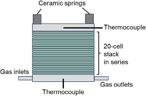
Figure 1. Schematic image of a 20-cell stack unit.

As depicted in Figure 2, the 20-cell stack unit (SOEC) was set in an electrical furnace (MAGNEX, SOFCECTS-3000), and the inlet gas ports were connected to each gas supply pipe. An H₂O–H₂ mixture was supplied to the fuel electrode, where steam was stably generated using an evaporator with precise flow control. This led to cell-voltage stability within ± 0.2 mV under electrolysis testing conditions. The flow rate of each gas was controlled using thermal mass-flow controllers (MFCs) (FUJIKIN FCS-T1000Z), which had been calibrated beforehand to achieve ±1.0% precision at set points within the used range. Current was controlled with direct-current (DC) power supply (KIKUSUI, PWX1500L) and measured using a precise 1 mΩ shunt resistor (Alpha electronics, PSBWR0010B). Measurement data such as cell voltage, temperatures, and flow rates were recorded using a portable recorder (YOKOGAWA, MV 2000).

Figure 2

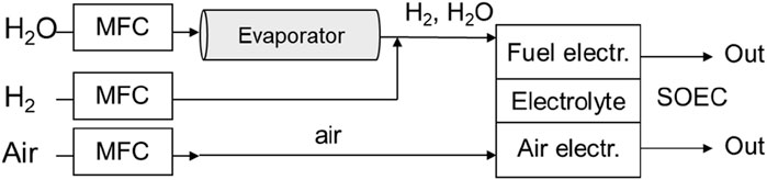
Figure 2. Twenty-cell-stack SOEC test equipment for steam electrolysis. MFC stands for thermal mass-flow controller.

The SOEC stack was heated in the furnace at a rate of 200 K/h with 10% H₂/N₂ for the fuel electrode and air for the other electrode at 20 standard liters per minute (SLM) for each. Once the stack temperature reached 650°C, the gases switched to 90% H₂O–H₂ for the fuel electrode (cathode) and air for the air electrode (anode). By maintaining constant steam utilization (U) at 80%, voltage–current density (V–J) characteristics were obtained by incrementally changing the current, where each current value was held for 2 min at 650°C, 700°C, 750°C, and 800°C, respectively. After the test, the average cell voltages were analyzed through multiple regression as a function of J and temperature (T). In this study, the furnace temperature was assumed to be the same as the stack temperature. A degradation test of the 20-cell stack was not performed in this study.

2.2 Process simulation method for the solar-heat-assisted SOEC system

A dynamic process simulation model (MathWorks, MATLAB/Simulink 2019b) was developed to analyze the solar-heat-assisted hydrogen production system with SOEC steam electrolysis (H₂O + 2e⁻ → H₂ + O²⁻, O²⁻ → 1/2O₂ + 2e⁻). Solar heat fluctuation was modeled with direct normal solar irradiation (DNI) data from Port Hedland, Australia, on a day in December and incorporated into the model. Figure 3 depicts the process-simulation model configuration. Fresh water was preheated using a heat exchanger (HEX) 3. The water was assumed to evaporate and turn into 600°C steam in the HEX 1. A preheater was used to control the gas mixture at the fuel-electrode (cathode) inlet at 730°C. An estimated 82% of steam was utilized for electrolysis (conversion rate). Approximately 12.5% of fuel offgas is recycled to the cathode inlet to supply hydrogen, resulting in 80% steam utilization in the SOEC. The final product, hydrogen, is obtained at 0°C after the removal of water using a chiller (coefficient of performance: 6.5) (Wajima et al., 2014).

Figure 3

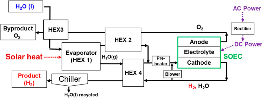
Figure 3. Process simulation model for the solar-heat-assisted SOEC system.

The experimental data on the 20-cell SOEC stack performance, as mentioned in Section 2.1, were assumed as a proxy for large-scale SOEC performance. Since there is a difference in the thermal boundary condition between the small 20-cell-stack and the 1-MW-class SOEC, the electrochemical performance of the 1 MW SOEC carries uncertainties that should be addressed in future work. In the process simulation, air supply to oxygen was omitted, while air supply was fed in the 20-cell stack experiment. Air supply may affect temperature distribution and the stack voltage in the SOEC stack. However, the experiment was carried out with pre-heated air to achieve isothermal testing conditions. Therefore, we assumed that the experimental data can be applied to numerical simulations.

The thermal mass of a repeat unit of SOEC was estimated to be 317 J/K (Wehrle et al., 2022), assuming 500 μm Ni–8YSZ, 10 μm 8YSZ, and 20 μm LSCF. Although the air-electrode material LSC in the experiment was different from that in the literature, we assumed that the change was negligible. Since the repeat unit number was 10,859, the total thermal mass of the SOEC stack was estimated to be 3.44 MJ/K. The temperature of the SOEC stack was calculated based not only on the energy balance among gas enthalpies at the inlet and outlet, input DC power, and heat loss to the atmosphere (9.7 kW at 750°C) but also on the thermal mass of the SOEC. In the 20-cell stack experiment, air was supplied to the air-electrode, while air was omitted in the process simulation to decrease air blower power and improve system efficiency.

Renewable electrical power for the SOEC was presumed to be supplied from the grid, with a rectifier efficiency of 95%. Power fluctuation was assumed to be the same as that of the solar heat. In the future, grid power availability should be investigated. In this study, an intraday simulation of the system was performed from approximately 6:00 to 18:00 to investigate how the solar-heat-assisted SOEC system can be controlled and how it respond over a short period as the first step. In future work, day-to-day and month-to-month system simulation will be carried out while considering night-time standby operation of the SOEC near 700°C.

2.3 Renewable resources and techno-economic analysis

Japan and Australia were analyzed for their solar energy resource potential and, therefore, the suitability for the implementation of a concentrated solar thermal energy process. All commercial concentrated solar thermal power plants are located in areas with an annual DNI of at least 2,000 kWh/m²/a (Buck and Schwarzbözl, 2018). Therefore, the location selection is based on the criteria of offering a DNI >2,000 kWh/m²/a. Western Australia and the region of Port Hedland show constant high probability of a DNI above 400 W/m² throughout the year, while other regions are affected more by seasonal changes and cloud-forming probabilities (Prasad et al., 2015). Furthermore, the location-specific DNI, generated using commercial software Meteonorm v8.2.0 (Meteotest AG, 2024), is used for an annual yield assessment and process optimization.

The levelized cost of hydrogen (LCOH₂) is the selected performance indicator assessing the techno-economic performance of the process. Additionally, the cost of fuel transportation to Tokyo by shipping it as liquefied H₂ (LH₂) is considered, which is added to the LCOH₂. First, the H₂ production cost by the solar thermal-powered SOEC is analyzed. Thereafter, the liquefaction and transportation costs are evaluated to capture the total H₂ costs in Japan. The LCOH₂ is calculated Equation 1 using the methodology presented by Albrecht et al. (2017) as follows:

${\text{LCOH}}_2=\frac{\text{ACC}+\text{OPEX}+{\mathrm{C}}_{\text{el}}+{\mathrm{C}}_{{\mathrm{H}}_2\mathrm{O}}}{{\mathrm{m}}_{{\mathrm{H}}_2}},(1)$

$\text{FCI}=\left(1+{\mathrm{f}}_{\text{add}}\right)\sum {\text{EC}}_{\mathrm{i}},(2)$

$\text{ACC}=\text{FCI}\frac{\mathrm{i}{\left(1+\mathrm{i}\right)}^{{\mathrm{n}}_{\text{Project}}}}{{\left(1+\mathrm{i}\right)}^{{\mathrm{n}}_{\text{Project}}}-1}.(3)$

The LCOH₂ Equation 1 includes the annual capital costs (ACCs), the operational expenditures (OPEX) concerning operational and maintenance costs, the electrical costs (${\mathrm{C}}_{\text{el}}$), and the costs for the continuous water demand (${\mathrm{C}}_{{\mathrm{H}}_2\mathrm{O}}$). All annual costs are divided by the annually produced hydrogen ($\left.{\mathrm{m}}_{{\mathrm{H}}_2}\right)$ to define the product-specific production costs. The ACC is calculated using the project duration (${\mathrm{n}}_{\text{Project}}$), the interest rate (i), and the fixed capital investment (FCI), which represents the equipment costs (ECs) and an additional project-related cost factor ($\left.{\mathrm{f}}_{\text{add}}\right)$ (Equation 2; Equation 3). The methodology described by Roeder et al. (2024) is used to estimate the total electrolysis system costs, including the investment costs for the stack replacements. Furthermore, the impact of SOEC degradation rates on energy efficiency and costs was analyzed, which showed a significant impact on the number of stack replacements and, therefore, the costs. Hence, ongoing stack development targets in terms of costs and degradation rates are considered.

The EC for the solar thermal system is included in the FCI, which takes the costs of the tower, the receiver, and the heliostat field into account. The tower cost of the solar concentration system is calculated according to Equation 4 using the tower height ${\mathrm{h}}_{\text{Tower}}$ as an input variable (Weinrebe et al., 2014). Furthermore, thermal energy storage (TES) can be integrated into the system. Therefore, the cost of the storage system is added to the ACC of the solar thermal system, and a storage capacity-specific cost factor of 40 USD/kWh_th is used (Dersch et al., 2021) together with a storage cycling efficiency of 85% to calculate the dischargeable energy content of the storage. The ECs are calculated using specific cost factors for individual components under the cost scenarios of 2023 and 2030 and are summarized in Table 1. In the 2030 scenario, a cost reduction of 25% is considered for solar thermal components. All costs are given in USD, and the CEPCI and a currency exchange rate of 1 USD = 0.90 € are used to convert all cost factors to 2023-equivalent USD costs.

${\text{EC}}_{\text{Tower}}=5.29{\mathrm{e}}^{0.006{\mathrm{h}}_{\text{Tower}}}\left[\text{MUSD}\right].(4)$

Table 1

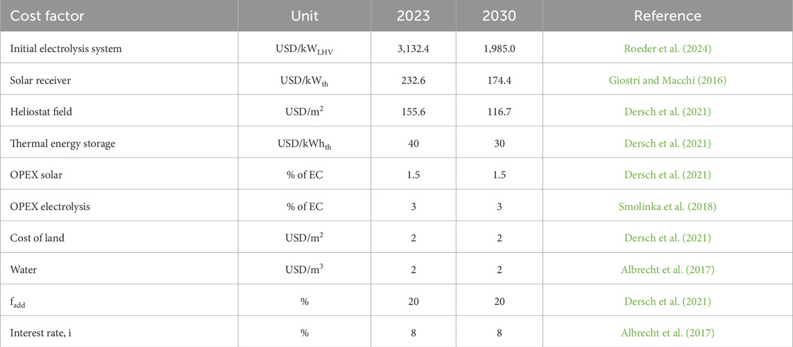
Table 1. Cost parameters for the techno-economic assessment.

For the accumulated annual electrical energy costs ${\mathrm{C}}_{\text{el}}$, the specific electrical energy demand of the process can is defined with Equation 5, where SOEC power is denoted as ${\mathrm{P}}_{\text{SOEC}}$, standby power is denoted as ${\mathrm{P}}_{\text{SOEC},\text{SB}}$, auxiliary power is denoted as ${\mathrm{P}}_{\text{AUX}}$, and additional power demand due to degradation is denoted as ${\mathrm{P}}_{\mathrm{DEG}}$.

${\mathrm{e}}_{{\mathrm{H}}_2}=\frac{\sum {\mathrm{P}}_{\text{SOEC}}\left(\mathrm{t}\right)+{\mathrm{P}}_{\text{SOEC},\text{SB}}\left(\mathrm{t}\right)+{\mathrm{P}}_{\text{AUX}}\left(\mathrm{t}\right)+{\mathrm{P}}_{\mathrm{DEG}}\left(\mathrm{t}\right)}{{\mathrm{m}}_{{\mathrm{H}}_2}},(5)$

Thus, the annual energy is calculated using the specific cost factor. According to the Clean Energy Council in Australia (Hugall et al., 2024), an average electricity price of 36–72 USD/MWh_el is achievable using wind and solar energy. Thus, we assume the mean value of 54 USD/MWh_el for the calculation of the annual electrical energy costs.

In the present study, a solar thermal intercept power of ${\dot{\mathrm{Q}}}_{\mathrm{INT}}=100$MW is considered for the reference case. The selected 100 MW is approximately an order of magnitude larger than the large-scale research facilities PSA (Plataforma Solar de Almería) and STJ (Solar Towers Jülich). Therefore, HFLCAL is used to calculate the tower height, the heliostat field efficiency, and the total number of heliostats needed (Schwarzbözl et al., 2009). The field layout is designed for 21 March, representing an annually averaged date in terms of solar resource utilization between the summer and winter seasons. Therefore, the equipment size of the solar thermal system is defined. Hence, the electrolysis scale in relation to ${\dot{\mathrm{Q}}}_{\mathrm{INT}}$ is economically optimized to achieve the lowest LCOH₂ by calculating the annual H₂ production yield. The chosen optimization algorithm is based on an efficient heuristic for global optimization (Storn and Price, 1997). The algorithm can adopt multiple decision variables of a problem (Guccione et al., 2022). In this study, electrolysis power is chosen as the decision variable to optimize for the lowest LCOH₂ because electrolysis is considered to contribute significantly to the total investment costs. The electrical power for electrolysis is, therefore, related to the thermal intercept power of the concentrated solar receiver using Equation A1. The optimization is conducted using the differential evolution algorithm of SciPy¹ in Python coding. For optimization, linear SOEC standby behavior is assumed. For example, if the available solar resource is only capable of providing 50% of the SOEC thermal power, we consider that 50% of the SOEC is operated at nominal conditions and the other 50% is in standby mode. By assuming a linear standby behavior, the minimal SOEC unit size is neglected, and the model is simplified. The equations provided in Table 2 are used for calculating the annual H₂ production rate depending on the solar resource.

Table 2

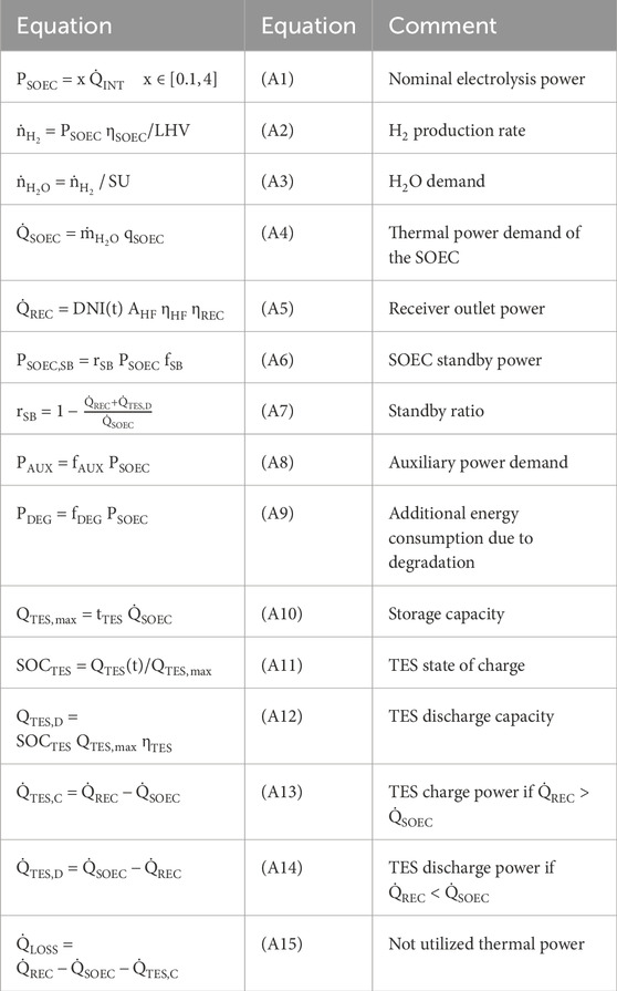
Table 2. Equations used for the annual yield calculation and techno-economic optimization.

Figure 4 shows the annual yield calculation and cost optimization using the differential evolution algorithm. The differential evolution algorithm optimizes the input variable x, which is equivalent to the electrolysis power until the lowest LCOH₂ is found. Thus, the nominal SOEC power is defined by this input value in relation to solar-intercepted power, as shown in Equation A1. The nominal H₂ production rate is calculated as shown in Equation A2 using the nominal electrolysis power, the stack efficiency ${\mathrm{\eta }}_{\text{SOEC}}$, and the LHV of hydrogen. Furthermore, the steam demand is defined by the ratio of the H₂ production rate and the steam utilization SU (A3), and the thermal energy demand to evaporate water to steam and superheat it to over 600 °C is defined by the specific thermal energy demand ${\mathrm{q}}_{\text{SOEC}}$ (A4). At every time-step, the thermal power output by the solar receiver is determined as shown in Equation A6 using the actual DNI, the size of the heliostat field ${\mathrm{A}}_{\text{HF}}$, and the efficiency of the heliostat field ${\mathrm{\eta }}_{\text{HF}}$ and receiver ${\mathrm{\eta }}_{\text{REC}}$. Therefore, the SOEC standby ratio ${\mathrm{r}}_{\text{SB}}$ is calculated depending on the receiver thermal output using Equation A7, which also includes the thermal output of TES, if applicable. Thus, the electrical standby power demand can be calculated as shown in Equation A6 using the nominal standby power factor ${\mathrm{f}}_{\text{SB}}.$ Similarly, the power demand by the auxiliary components is calculated with the specific power demand ${\mathrm{f}}_{\text{AUX}}$ using Equation A8. The additional electrical energy demand due to degradation is considered as shown in Equation A9. The end-of-life of an electrolysis stack is reached when its electrical energy demand is increases by 10%, according to the European Commission (European Commission—Clean Hydrogen JointUndertaking, 2022), and therefore, a degradation factor ${\mathrm{f}}_{\mathrm{DEG}}=0.05$ is applied. The analysis of the process, including the TES, is carried out using Equations A10–A14, calculating the maximum storage capacity with a storage discharge duration of ${\mathrm{t}}_{\text{TES}}=12\mathrm{h}$ and ${\dot{\mathrm{Q}}}_{\text{SOEC}}$. Thus, the state of charge (${\text{SOC}}_{\text{TES}}$) can be defined at any given time when the TES is charged ${\dot{\mathrm{Q}}}_{\text{TES},\mathrm{C}}$ or discharged ${\dot{\mathrm{Q}}}_{\text{TES},\mathrm{D}}$. Therefore, it will be differentiated by assessing the availability of thermal receiver power in comparison to the SOEC demand. Furthermore, the storage capacity during discharge is affected by TES cycling efficiency ${\mathrm{\eta }}_{\text{TES}}$ as it is affected by losses. To define solar energy utilization, the non-utilized power is calculated using Equation A15. Electrolysis power is adjusted using the optimization algorithm, while the solar thermal system is the same. Hence, the utilization rate can be calculated by dividing the annually non-utilized energy by the total thermal energy output of the receiver.

Figure 4

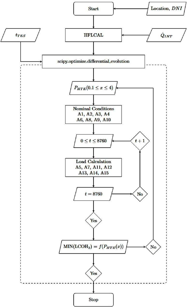
Figure 4. Flow chart of the annual H₂ yield calculation and cost optimization algorithm.

With the assessment of the solar thermal SOEC process, the annual H₂ is known, and therefore, the daily production rate is estimated. For the H₂ liquefaction process, the investment and operational costs are based on the values reported by Niermann et al. (2021). The investment cost is adjusted by a scaling factor of 0.66 to the reference scale of 30 kg/h. Additionally, a specific electrical energy demand of 6.78 kWh/kg and an operation and maintenance cost share of 8% on the equipment cost are used. Furthermore, 1.65% H₂ loss during the liquefaction process is reasonable (Niermann et al., 2021). The lifetime of the liquefaction process is assumed to be 25 years, which is equal to the solar thermal process components. For the LH₂ transport, a cost factor of 0.0488 USD/kg per 1,000 km of transport distance is used for the assessment (ERIA, 2020). During the transportation and storage phase of H₂, a boil-off rate in the range of 0.1%–0.3% can occur for large-scale storage tanks (Berstad et al., 2022). Furthermore, no cost developments are considered for the future cost outlook of the liquefaction and transportation processes. Economic assessment is only conducted for different process configurations with and without TES, and a cost-sensitivity analysis is conducted for the electrical energy price (36–72 USD/MWh_el), the interest rate (5%–10%), and all other CAPEX and OPEX (±10%). By summing up the H₂ losses during the liquefaction, storage, and transportation period, the total loss is calculated to be in the range of 2.5%–7.5%. The cost impact of potential H₂ losses is analyzed through a sensitivity study.

3 Results and discussion

3.1 Low-cost renewable energy resources for Japan

The highest annual DNI of Japan is approximately 1,500 kWh/m²/a, while in Australia, the DNI can be twice as high, reaching 2,900 kWh/m²/a. Japan lies between 30° north and 45° north, while Australia lies between 10° south and 40° south. In the coastal region of Australia at 40° south, the annual DNI values are similar to those in Japan. Thus, the difference in DNI can be mainly attributed to the distance from the equator and the increased diffuse solar radiation caused by generally cloudier sky near the sea. For concentrated solar thermal systems, a DNI above 1,800–2,000 kWh/m²/a is considered economically optimal (Buck and Schwarzbözl, 2018). Therefore, Australia—more specifically, Western Australia—is suitable for the cost-effective use of concentrated solar energy. Hence, a location near Port Hedland in Western Australia was selected for the detailed analysis. The daily DNI at Port Hedland over a full year, used for the process simulation and techno-economic assessment, is based on data from Meteonorm v8.2.0 (Meteotest AG, 2024). Due to its proximity to the equator at 20.8° south, only a small seasonal variance is observed. This results in an annual DNI of 2,543 kWh/m²/a. With the site selected, the heliostat field layout is calculated using HFLCAL (Schwarzbözl et al., 2009).

Figure 5 shows the resulting heliostat field layout for a 100 MW solar thermal intercept power. The field is located in the south, concentrating the incoming solar irradiation on the northern tower. Additionally, the field is only on one side of the tower because a cavity receiver is required to achieve high temperatures. Therefore, the annual heliostat field efficiency is 61.1% using 3,246 heliostats. Each colored circle represents a heliostat. The heliostats marked in red are currently covered by the shadow of the tower marked in black. The annual solar-to-thermal efficiency is 51.9%, assuming an average receiver efficiency of 85%. Thus, the thermal power transferred to the heat transfer medium is 85 MW. Therefore, a total land area of approximately 1,000,000 m² is required, with a heliostat surface area of 168,305 m².

Figure 5

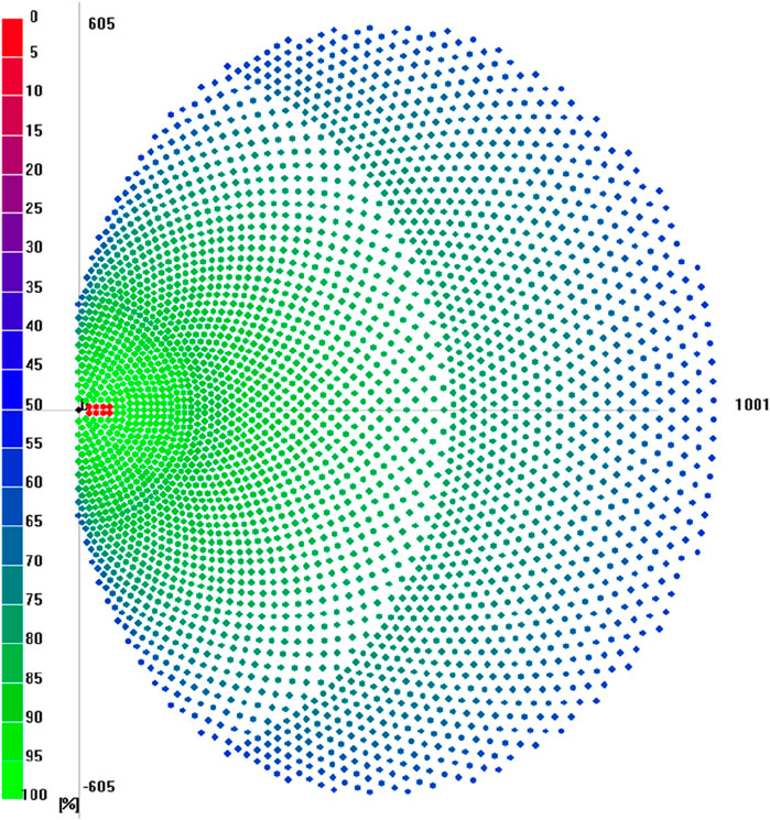
Figure 5. Heliostat field layout for an intercept power of 100 MW in Port Hedland, Australia, with a total of 3,246 heliostats.

3.2 Performance evaluation of the solar-heat-assisted SOEC system for hydrogen production

A 20-cell SOEC stack was tested at constant 80% steam utilization to evaluate stack voltage–current density and DC power and current density relationships at 650 ºC–800°C. As shown in Figure 6, higher electrolysis temperatures led to lower cell voltages, which indicates higher performance. Approximately 1.5 kW DC input was observed at 0.7 A/cm². The average cell voltages (V_cell) were analyzed via multiple regressions. This yielded V_cell (V) = 1.903551 + 0.562342 J −0.00088 T as a function of current density (J) and absolute temperature of SOEC (T) with ±4% error.

Figure 6

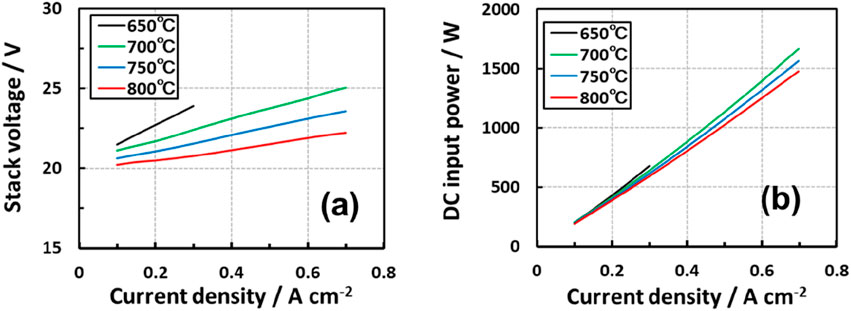
Figure 6. (a) Stack voltage vs. current density and (b) DC input power vs. current density curves for the 20-cell stack. Steam utilization was constant at 80%.

Dynamic process simulation was carried out to analyze the solar-heat-assisted hydrogen production system via SOEC steam electrolysis (H₂O → H₂ + 1/2O₂). A thermal mass of the 1 MW-class SOEC stack was considered. Solar heat fluctuation was modeled using DNI data from Port Hedland and incorporated into the model (see Figure 7a). Steam at 600°C is assumed to be instantly generated, and 82% of the steam was utilized for electrolysis (conversion rate). Recycling 12.5% fuel offgas led to 80% utilization of steam in the SOEC stack. Experimental data on 20-cell SOEC stack performance (voltage–current density characteristics) were presumed to be the same as those of a large-scale SOEC (see Figure 6a).

Figure 7

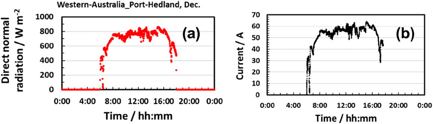
Figure 7. (a) DNI data from Port Hedland in December and (b) input current to the SOEC stack.

Numerical simulation on the 1 MW-class SOEC with solar heat for steam generation was implemented to keep the steam utilization constant even though the input solar power fluctuated. The input renewable power profile was assumed to be the same as that of DNI. At the maximum DNI points, input power and water were also maximized. As exhibited in Figure 7b, the electrolysis current was obtained according to the DNI profile. Solar heat generation and steam electrolysis responded to fluctuations in input heat and electrical power. As displayed in Figure 8a, DC power input to the SOEC stack was maximized to 916 kW. At this point, input solar heat was estimated to be 139 kW. Therefore, solar heat can save 12% more electric power than conventional hydrogen production with SOECs. Furthermore, utilization of exhausted oxygen heat for preheating water (HEX 3 in Figure 3) saved input solar power by 20%.

Figure 8

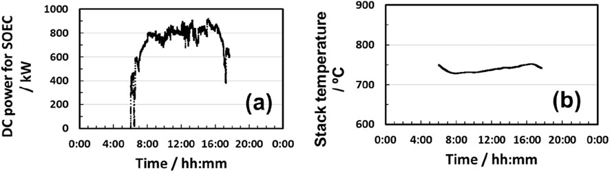
Figure 8. (a) DC power input into the SOEC stack and (b) SOEC-stack temperature deviation.

As shown in Figure 8b, a flat SOEC stack temperature profile was obtained at 729 ºC–751°C with relatively small deviations since the inlet gas temperature was controlled at 730°C. The pre-heating strategy will be effective for fluctuating power and heat operation. Figure 9 reveals that energy efficiency (electrical + thermal power to H₂) reached 92% on average (higher heating value (HHV) and alternating current base (AC)). The efficiency deviated from 90% to 99% mostly. These results suggest that energy efficiency can be maintained at 90% or higher, even under fluctuating input from renewable power sources. The total input amount of solar thermal and electrical energy was 756 kWh and 9,189 kWh, respectively, to obtain 252 kg of hydrogen during the day. Hence, the solar-heat-assisted SOEC system can be considered one of the efficient technologies for hydrogen production

Figure 9

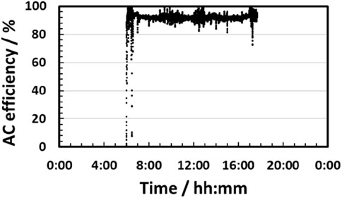
Figure 9. Alternating-current efficiency profile for the solar-heat-assisted SOEC system.

Furthermore, a cold-start of the system was simulated by assuming that heating of the SOEC starts at 6:00 a.m. using 600°C steam, with preheating from 25°C until the SOEC temperature reaches 650°C. The SOEC stack thermal mass is equivalent to 3.44 MJ/K, so it took 10.3 h for the start of electrolysis, and thermal input of 2.15 GJ and electrical input of 0.3 GJ were consumed during the heat-up process. In this case, the period of steam electrolysis operation will be limited to only 2 h during the day due to the long heating time of the SOEC stack. Only 26.1 kg of hydrogen was produced with an input electricity of 946 kWh over the last 2 h. In addition, cooling down of the SOEC will take longer than heating due to the assumed excellent thermal insulation. Therefore, daily cold-start and shutdown will not be applicable and economical. Hence, hot-standby of the SOEC stack at approximately 750°C at night will be realistic with less electricity consumption (10 kW for the 1 MW-class SOEC).

Based on the above results, the SOEC system will respond to the dynamic change in input solar heat and electrical power to attain average efficiency above 90%. Night-time standby operation of the system will consume 10 kW (AC) to maintain the SOEC stack at 750°C.

3.3 Techno-economic analysis of hydrogen production using the SOEC system

The results of the experimental investigation and simulation are used in the economic assessment. Table 3 summarizes the LCOH₂ of the economically optimized solar thermal-powered SOEC with and without TES for 2023 and 2030 starting projects. The table shows the achieved process full-load hours t_FLH, specific electrical energy demand ${\mathrm{e}}_{{\mathrm{H}}_2}$, the SOEC to solar-intercepted power ratio P_SOEC/ ${\dot{\mathrm{Q}}}_{\mathrm{INT}}$, and thermal losses Q_LOSS in relation to the annually collected solar thermal energy of the receiver Q_REC.

Table 3

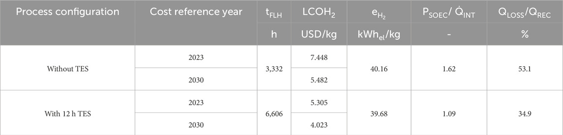
Table 3. Simulation results of the techno-economic-optimized H₂ production process with and without thermal energy storage.

In both cases, with and without TES, the solar thermal system is the same and achieves a solar thermal intercept power of 100 MW. The cost of the system and the solar thermal energy captured are the same in all cases. The SOEC power of the cost-optimized case is equal to 1.62 times the solar intercept power when no TES is used. The ratio is reduced to a factor of 1.09 when installing a storage capacity of 12 h. Higher ratios would reduce thermal losses and maximize the H₂ production rate. However, this would lead to an increase in investment costs and a decrease in ${\mathrm{t}}_{\text{FLH}}$ as the stack would be operated more often in partial load, increasing the standby electrical energy consumption. Therefore, LCOH₂ would increase. When implementing TES, the electrolysis capacity is smaller than in the case without TES. The investment cost of the electrolysis can, therefore, be reduced, and the operating hours at nominal conditions are increased for the lowest LCOH₂.

Figure 10 shows the LCOH₂ cost construction of the production process for the different cases and the cost scenario for 2023 and 2030. The cost impact of electrical energy consumption is approximately 2.10 to 2.13 USD/kg for the investigated cases as the specific electrical energy demand is at 39.68 and 40.16 kWh_el/kg for the case with and without 12 h thermal energy storage, respectively. Other relevant electrolyzer technologies have a specific electrical energy demand of 50 kWh_el/kg–55 kWh_el/kg for PEM and alkaline electrolyzers (Roeder et al., 2024). The cost contribution of the SOEC investment is 3.54 USD/kg at 3,332 h/year, which is higher than the 1.79 USD/kg at 6,606 h/year for the projects starting in 2023. However, only one stack replacement is required at the lower operating hours, while three are needed at over 6,500 h. Furthermore, one and two stack replacements are required for the process without and with TES, respectively, for the projects starting in 2030. The reduction in the number of stack replacements in the high t_FLH case is due to the ongoing SOEC developments and, therefore, lifetime improvements. The resulting specific investment costs for the SOEC system, including stack replacements, are 3,355.21 USD/kW_LHV and 3,832.42 USD/kW_LHV for projects starting in 2023. For projects starting in 2030, the costs are reduced to 2,073.29 USD/kW_LHV and 2,206.73 USD/kW_LHV, respectively. The higher costs are associated with the system using 12 h TES, which achieves higher process full-load hours. The higher annual operating full-load hours cause an earlier stack replacement, which is costlier.

Figure 10

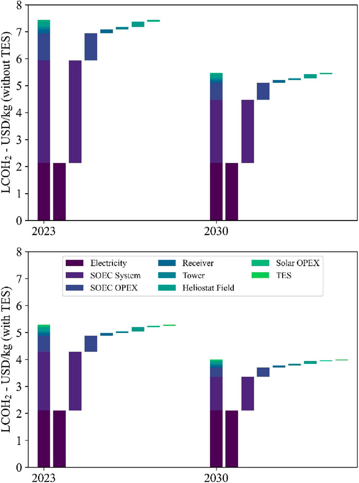
Figure 10. Levelized costs of hydrogen and cost composition of the H₂ production process for the investigated cases and the 2023 and 2030 cost scenarios.

The specific electrical energy demand of the process is calculated as follows:

${\mathrm{e}}_{{\mathrm{H}}_2}=\frac{\text{LHV}}{{{\mathrm{\eta }}_{\text{SOC}}\mathrm{\eta }}_{\text{AC}/\text{DC}}}\left(\frac{{\mathrm{f}}_{\text{SB}}\left(8760-{\mathrm{t}}_{\text{FLH}}\right)}{{\mathrm{t}}_{\text{FLH}}}+1+\frac{{\mathrm{f}}_{\mathrm{DEG}}}{2}+{\mathrm{f}}_{\text{AUX}}\right),(6)$

with the standby energy fraction (${\mathrm{f}}_{\text{SB}}$) as a function of the process full-load hours (${\mathrm{t}}_{\text{FLH}}$), the SOC efficiency (${\mathrm{\eta }}_{\text{SOC}}$), the fraction of the increased power at the end of stack life due to degradation (${\mathrm{f}}_{\mathrm{DEG}}$), and the electrical energy demand factor for all auxiliary components ${\mathrm{f}}_{\text{AUX}}$. Figure 11 shows Equation 6 plotted against the specific electrical energy demand of the optimized cases with and without 12 h TES. Therefore, Equation 6 can be used to evaluate the production and, thus, the economic potential of an SOEC with any type of electrical source as a function of process full-load hours. Furthermore, the equation can be used to compare different SOEC systems, including the electrical energy demand of the auxiliary components, the standby demand, and the degradation.

Figure 11

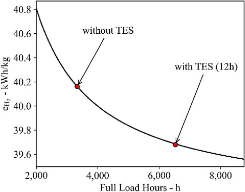
Figure 11. Specific electrical energy demand as a function of process full-load hours.

Table 4 summarizes the annual and, therefore, the daily H₂ production rate of the different process configurations. Furthermore, the specific investment costs of the liquefaction process are also given, considering a scaling factor of 0.66. For the liquefaction rate, a simultaneous operation with the SOEC is assumed and calculated by dividing the annual H₂ production rate by the achievable process full-load hours from Table 4. Although the annual production rate of the process using a TES is higher, the liquefaction rate is lower because of the smaller electrolysis capacity and higher process full-load hours. The liquefaction unit, therefore, achieves a higher capacity factor. The capital costs, the specific energy demand, and the share of operation and maintenance cost contribute to the mass-specific cost of H₂ and result in an additional an increase of 0.361 USD/kg and 0.362 USD/kg for the liquefaction process in the two configurations with and without TES, respectively. More than 99% of the mass-specific cost is due to the electrical energy demand of the liquefaction process.

Table 4

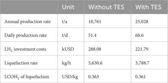
Table 4. Techno-economic results of the liquefaction process depending on the annual and, therefore, the daily H₂ production rate.

The distance between Port Hedland in Australia and the main island of Japan is approximately 9,000 km, and up to 75 tons of LH₂ can be transported per ship (Ratnakar et al., 2021). Therefore, we can calculate a cost impact of 0.439 USD/kg, which is added to the final H₂ production cost. The total LCOH₂ including the production in Western Australia, liquefaction, and transport to Japan, is shown in Table 5 for processes with and without TES, under the 2023 and 2030 cost scenarios. The production cost share is broken down into the SOEC, solar system, and TES contributions. The cost fraction of the different parts of each system is also shown. The highest cost share is allocated to the H₂ production system. When considering boiling-off losses in the range of 2.5%–7.5% of H₂ during liquefaction, storage, and transportation, the LCOH₂ increases equivalently to the loss of product.

Table 5

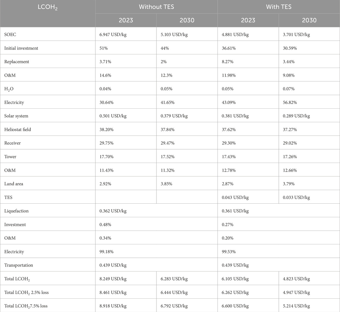
Table 5. Total techno-economic results of the solar-heat-supported SOEC process, including the transportation of LH₂ from the production site to Japan.

The production cost of the investigated process is reduced by implementing thermal energy storage as it increases the total operating hours at full-load. Previous studies of similar concepts show higher hydrogen production costs (Lin and Haussener, 2017; Mastropasqua et al., 2020). The present study considers the integration of grid electrical energy supply, which benefits from cost-optimized renewable energy supply from different sources. The electricity price is expected to be in the range of 36 USD/MWh–72 USD/MWh. Hence, Figure 12 shows the H₂ cost sensitivity due to electrical energy price changes compared to the reference case that assumes 54 USD/MWh_el. Therefore, the electrical energy accounts for the demand of the electrolysis system, according to Equation 6, and includes the specific electrical energy demand for the liquefaction process, which is 6.78 kWh_el/kg. Even for the considerably small electrical energy price change of ±18 USD/MWh_el, the LCOH₂ is expected to vary by ±0.845 to ±0.836 USD/kg for the two investigated cases.

Figure 12

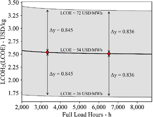
Figure 12. LCOH₂ sensitivity due to electrical energy price changes from 36 USD/MWh to 72 USD/MWh.

While the electrical energy demand can account for more than 30% of the H₂ costs, the remaining 70% is mainly caused by the capital expenditure.

Figure 13 shows the relative change in LCOH₂ for a relative change of different cost-impact factors. Changing the interest to 5% or 10% from the initial 8% has the biggest cost-change potential. The second- and third-biggest impacts are caused by changes in the electrical energy price and the SOEC investment and O&M costs. The cost for the solar system affected LCOH₂ the least as it only contributed to the thermal energy supply and accounted for only 15% of the total energy demand. However, a percentage change in electricity price of ±10% is equal to a change in levelized costs of electricity (LCOE) of ±5.4 USD/MWh. Therefore, a relative change in LCOH₂ of ±2.8% to ±5.5% with a higher impact on the case with a 12 h TES is identified. The price sensitivity used previously, i.e., an LCOE of 54 USD/MWh ±18 USD/MWh, is a 33% change in LCOE. Hence, the relative change in LCOH₂ can be as high as ±15% in the impact range of the interest rate. The reduction in the interest rate from 8% to 5% causes a reduction of −1.03 USD/kg and −0.60 USD/kg for the process without TES and projects starting in 2023 and 2030, respectively. Increasing the interest rate to 10% will cause an increase of +0.75 USD/kg and +0.47 USD/kg for the same process and project starting years. The change in interest rate to 5%, for a process with 12 h TES, results in a cost change of −0.62 USD/kg and −0.37 USD/kg for projects starting in 2023 and 2030, respectively. An increase to a 10% interest rate results in a cost change of +0.45 USD/kg and +0.27 USD/kg for the same project starting years later. The process without any TES is affected more by a change in the interest rate as the production capacity is limited by the achievable full-load hours. In contrast, when a 12 h TES is integrated into the process, full-load hours increase, and therefore, the impact of the capital expenditures is reduced. In contrast, the use of storage results in greater cost sensitivity in 2030 than in 2023 when electrical energy prices vary. This is due to the fixed electricity price of 54 USD/MWh used as the base case for both 2023 and 2030.

Figure 13

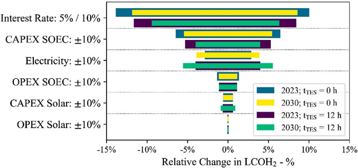
Figure 13. Tornado diagram for the cost sensitivity for the different cost-impact factors for the two different cases in 2023 and 2030.

Thus, the proposed solar-heat-integrated solid oxide electrolysis process is capable of generating hydrogen, produced in Australia and transported to Japan, at a price below 4 USD/kg for projects starting in 2030, considering the cost reduction potential from the sensitivity study. For the comparison of H₂ production costs between the presented concentrated solar-powered SOEC and a PEM electrolysis system, the same electrolysis investment cost calculation method is used for the SOEC and the PEM electrolysis system (Roeder et al., 2024). The H₂ production costs of the PEM electrolysis system will be cheaper, except for the future costs outlook in 2030 at 6,606 process full-load hours. In this case, the H₂ production costs are almost cost equivalent, 4.145 USD/kg using PEM electrolysis compared to 4.023 USD/kg for the SOEC system, including the costs of the solar thermal and thermal storage system. The SOEC will be cost-competitive in future due to the cost reduction potential and low-cost heat-integration possibilities.

4 Conclusion

For low-cost RE and hydrogen production, we conclude that Australia is an optimal region for hydrogen exportation to Japan in terms of distance and solar irradiance. Concentrated solar systems should be installed in areas with high (DNI because only direct sunlight can be concentrated, and therefore, cloudy areas are less suitable. For the investigated process, a reference scale of 100 MW solar thermal intercepting power with an appropriately sized SOEC system was investigated. The developed dynamic process simulation model resulted in an average energy efficiency (electrical + thermal to H₂) of 92% for a 1 MW-class SOEC. The reference-scale 100 MW plant achieved an annual average solar-to-thermal conversion efficiency of 51.9%. The process, therefore, requires a total land area of 1,000,000 m² to collect the incoming solar radiation and concentrate it on a central receiver. As a result, the unit cost of 1 kg of H₂ ranges from 6.105 USD/kg to 8.249 USD/kg for a system with and without thermal energy storage, respectively, both including liquefaction of H₂ and its transport from Australia to Japan. In the future, the costs are expected to decrease to 4.823 USD/kg and 6.283 USD/kg for projects starting in 2030, mainly due to a reduction in the cost of the SOEC system. The H₂ production costs can be further reduced to less than 4.0 USD/kg with lower energy prices and lower interest rates. In the future, reductions in SOEC costs and H₂ boiling-off losses are expected to lower the total hydrogen cost below that of the on-going coal-based H₂ production with CCU and transportation to Japan.

Data availability statement

The raw data supporting the conclusions of this article will be made available by the authors, without undue reservation.

Author contributions

YT: Data curation, Funding acquisition, Investigation, Methodology, Project administration, Writing – original draft, Writing – review and editing. TR: Data curation, Investigation, Methodology, Writing – original draft, Writing – review and editing, Software. NM: Funding acquisition, Project administration, Supervision, Writing – review and editing.

Funding

The author(s) declare that financial support was received for the research and/or publication of this article. This article was financially supported by the National Institute of Advanced Industrial Science and Technology and the German Aerospace Center.

Conflict of interest

The authors declare that the research was conducted in the absence of any commercial or financial relationships that could be construed as a potential conflict of interest.

Generative AI statement

The author(s) declare that no Generative AI was used in the creation of this manuscript.

Publisher’s note

All claims expressed in this article are solely those of the authors and do not necessarily represent those of their affiliated organizations, or those of the publisher, the editors and the reviewers. Any product that may be evaluated in this article, or claim that may be made by its manufacturer, is not guaranteed or endorsed by the publisher.

Footnotes

¹https://docs.scipy.org/doc/scipy/reference/generated/scipy.optimize.differential_evolution.html

References

Albrecht, F. G., König, D. H., Baucks, N., and Dietrich, R.-U. (2017). A standardized methodology for the techno-economic evaluation of alternative fuels – a case study. Fuel 194, 511–526. doi:10.1016/j.fuel.2016.12.003

CrossRef Full Text | Google Scholar

Alzahrani, A. A., and Dincer, I. (2016). Design and analysis of a solar tower based integrated system using high temperature electrolyzer for hydrogen production. Int. J. Hydrogen Energy 41, 8042–8056. doi:10.1016/j.ijhydene.2015.12.103

CrossRef Full Text | Google Scholar

Arashi, H., Naito, H., and Miura, H. (1991). Hydrogen production from high-temperature steam electrolysis using solar energy. Int. J. Hydrogen Energy 16 (9), 603–608. doi:10.1016/0360-3199(91)90083-u

CrossRef Full Text | Google Scholar

Berstad, D., Gardarsdottir, S., Roussanaly, S., Voldsund, M., Ishimoto, Y., and Nekså, P. (2022). Liquid hydrogen as prospective energy carrier: a brief review and discussion of underlying assumptions applied in value chain analysis. Renew. Sustain. Energy Rev. 154, 111772. doi:10.1016/j.rser.2021.111772

CrossRef Full Text | Google Scholar

Buck, R., and Schwarzbözl, P. (2018). “4.17 solar tower systems,” in Comprehensive energy systems (Elsevier), 692–732.

CrossRef Full Text | Google Scholar

Dersch, J., Paucar, J., Schuhbauer, C., Schweitzer, A., and Stryk, A. (2021). Blueprint for molten salt CSP power plant: final report of the research project. CSP-Reference Power Plant “Made in Germany. doi:10.1063/5.0085877

CrossRef Full Text | Google Scholar

ERIA (2020). Review of hydrogen transport cost and its perspective (liquefied hydrogen) Available online at: https://www.eria.org/uploads/media/Research-Project-Report/RPR_2020_16/11_Chapter-4-Review-of-Hydrogen-Transport-Cost-_(Liquefied-Hydrogen)_801.pdf (Accessed 12 October 2024).

Google Scholar

European Commission - Clean Hydrogen Joint Undertaking (2022). Strategic research and innovation agenda 2021 – 2027, european commission - Clean hydrogen joint undertaking. Available online at: https://www.clean-hydrogen.europa.eu/knowledge-management/sria-key-performance-indicators-kpis_en (Accessed February 8, 2023).

Google Scholar

Giostri, A., and Macchi, E. (2016). An advanced solution to boost sun-to-electricity efficiency of parabolic dish. Sol. Energy 139, 337–354. doi:10.1016/j.solener.2016.10.001

CrossRef Full Text | Google Scholar

Guccione, S., Trevisan, S., Guedez, R., Laumert, B., Maccarini, S., and Traverso, A. (2022). “Techno-economic optimization of a hybrid PV-CSP plant with molten salt thermal energy storage and supercritical CO2 brayton power cycle,”. Cycle innovations; cycle innovations (Rotterdam, Netherlands), 4, GT2022–80376.Energy Storage. doi:10.1115/GT2022-80376

CrossRef Full Text | Google Scholar

Houaijia, A., Breuer, S., Thomey, D., Brosig, C., Säck, J.-P., Roeb, M., et al. (2014). Solar hydrogen by high-temperature electrolysis: flowsheeting and experimental analysis of a tube-type receiver concept for superheated steam production. Energy Procedia 49, 1960–1969. doi:10.1016/j.egypro.2014.03.208

CrossRef Full Text | Google Scholar

Hugall, I., Lee, K., Pinnegar, M., Son, A., and Wymond, B. (2024). Lelevised cost of electricity - review. Clean. Energy Counc. Available online at: https://cleanenergycouncil.org.au/getmedia/2c81080a-cd54-4845-904e-4846606c26cf/levelised-cost-of-electricity-review.pdf (Accessed September 10, 2024).

Google Scholar

IRENA (2024). Green hydrogen strategy: a guide to design. Int. Renew. Energy Agency.

Google Scholar

Kadohiro, Y., Risthaus, K., Monnerie, N., and Sattler, C. (2024). Numerical investigation and comparison of tubular solar cavity receivers for simultaneous generation of superheated steam and hot air. Appl. Therm. Eng. 238, 122222. doi:10.1016/j.applthermaleng.2023.122222

CrossRef Full Text | Google Scholar

Kadohiro, Y., Roeder, T., Risthaus, K., Laaber, D., Monnerie, N., and Sattler, C. (2025). Experimental demonstration and validation of tubular solar cavity receivers for simultaneous generation of superheated steam and hot air. Appl. Energy 380, 125042. doi:10.1016/j.apenergy.2024.125042

CrossRef Full Text | Google Scholar

Kadohiro, Y., Thanda, V. K., Lachmann, B., Risthaus, K., Monnerie, N., Roeb, M., et al. (2023). Cavity-shaped direct solar steam generator employing conical helical tube for high-temperature application: model development, experimental testing and numerical analysis. Energy Convers. Manag. X 18, 100366. doi:10.1016/j.ecmx.2023.100366

CrossRef Full Text | Google Scholar

Lin, M., and Haussener, S. (2017). Techno-economic modeling and optimization of solar-driven high-temperature electrolysis systems. Sol. Energy 155, 1389–1402. doi:10.1016/j.solener.2017.07.077

CrossRef Full Text | Google Scholar

Lin, M., Suter, C., Diethelm, S., van Herle, J., and Haussener, S. (2022). Integrated solar-driven high-temperature electrolysis operating with concentrated irradiation. Joule 6 (9), 2102–2121. doi:10.1016/j.joule.2022.07.013

CrossRef Full Text | Google Scholar

Ma, Z., and Martinek, J. (2024). ‘Integration of concentrating solar power with high temperature electrolysis for hydrogen production', SolarPACES Conf. Proc., SolarPACES Conf. Proc., 2. doi:10.52825/solarpaces.v2i.973

CrossRef Full Text | Google Scholar

Martins, J. H. S., Roeder, T., Rosenstiel, A., and Monnerie, N. (2024). “Solar hydrogen production: techno-economic evaluation of concentrated solar power plant and high-temperature electrolysis integration”, Int. Sol. Energy Soc., 1–13. doi:10.18086/eurosun.2024.09.05

CrossRef Full Text | Google Scholar

Mastropasqua, L., Pecenati, I., Giostri, A., and Campanari, S. (2020). Solar hydrogen production: techno-Economic analysis of a parabolic dish-supported high-temperature electrolysis system. Appl. Energy 261, 114392. doi:10.1016/j.apenergy.2019.114392

CrossRef Full Text | Google Scholar

Meteotest AG (2024). Meteonorm (V8.2.0). Available online at: https://meteonorm.com/.

Google Scholar

Mohammadi, A., and Mehrpooya, M. (2019). Thermodynamic and economic analyses of hydrogen production system using high temperature solid oxide electrolyzer integrated with parabolic trough collector. J. Clean. Prod. 212, 713–726. doi:10.1016/j.jclepro.2018.11.261

CrossRef Full Text | Google Scholar

Monnerie, N., von Storch, H., Houaijia, A., Roeb, M., and Sattler, C. (2017). Hydrogen production by coupling pressurized high temperature electrolyser with solar tower technology. Int. J. Hydrogen Energy 42, 13498–13509. doi:10.1016/j.ijhydene.2016.11.034

CrossRef Full Text | Google Scholar

Niermann, M., Timmerberg, S., Drünert, S., and Kaltschmitt, M. (2021). 'liquid organic hydrogen carriers and alternatives for international transport of renewable hydrogen. Renew. Sustain. Energy Rev. 135, 110171. doi:10.1016/j.rser.2020.110171

CrossRef Full Text | Google Scholar

Prasad, A. A., Taylor, R. A., and Kay, M. (2015). Assessment of direct normal irradiance and cloud connections using satellite data over Australia. Appl. Energy 143, 301–311. doi:10.1016/j.apenergy.2015.01.050

CrossRef Full Text | Google Scholar

Puig-Samper, G., Bargiacchi, E., Iribarren, D., and Dufour, J. (2022). Assessing the prospective environmental performance of hydrogen from high-temperature electrolysis coupled with concentrated solar power. Renew. Energy 196, 1258–1268. doi:10.1016/j.renene.2022.07.066

CrossRef Full Text | Google Scholar

Ratnakar, R. R., Gupta, N., Zhang, K., van Doorne, C., Fesmire, J., Dindoruk, B., et al. (2021). Hydrogen supply chain and challenges in large-scale LH2 storage and transportation. Int. J. Hydrogen Energy 46 (47), 24149–24168. doi:10.1016/j.ijhydene.2021.05.025

CrossRef Full Text | Google Scholar

Roeder, T., Rosenstiel, A., Monnerie, N., and Sattler, C. (2024). Impact of expected cost reduction and lifetime extension of electrolysis stacks on hydrogen production costs. Int. J. Hydrogen Energy 95, 1242–1251. doi:10.1016/j.ijhydene.2024.08.015

CrossRef Full Text | Google Scholar

Schiller, G., Lang, M., Szabo, P., Monnerie, N., Storch, H. von, Reinhold, J., et al. (2019). Solar heat integrated solid oxide steam electrolysis for highly efficient hydrogen production. J. Power Sources 416, 72–78. doi:10.1016/j.jpowsour.2019.01.059

CrossRef Full Text | Google Scholar

Schwarzbözl, P., Schmitz, M., and Pitz-Paal, R. (2009). “Visual HFLCAL - a software tool for layout and optimisation of heliostat fields,” in SolarPACES 2009.

Google Scholar

Smolinka, T., Wiebe, N., Sterchele, P., Palzer, A., Lehner, F., Jansen, M., et al. (2018). Studie: IndWEDe Industrialisierung der Wasser-elektrolyse in -Deutschland: -chancen und -Herausforderungen für nachhaltigen Wasserstoff für Verkehr, Strom und -Wärme. Available online at: https://www.ise.fraunhofer.de/de/veroeffentlichungen/studien/indwede.html (Accessed December 22, 2023).

Google Scholar

Storn, R., and Price, K. (1997). Differential evolution – a simple and efficient heuristic for global optimization over continuous spaces. J. Glob. Optim. 11 (4), 341–359. doi:10.1023/a:1008202821328

CrossRef Full Text | Google Scholar

Wajima, K., Hasegawa, Y., Hasegawa, O., Koga, J., and Yawata, N. (2014). “GART Series” large capacity centrifugal chillers achieved high efficiency, downsizing. Mitsubishi Heavy Ind. Tech. Rev. 51 (2), 26–31. Available online at: https://www.mhi.com/technology/review/sites/g/files/jwhtju2326/files/tr/pdf/e512/e512026.pdf.

Google Scholar

Wehrle, L., Wang, Y., Boldrin, P., Brandon, N. P., Deutschmann, O., and Banerjee, A. (2022). Optimizing solid oxide fuel cell performance to Re-evaluate its role in the mobility sector. ACS Environ. 2, 42–64. doi:10.1021/acsenvironau.1c00014

PubMed Abstract | CrossRef Full Text | Google Scholar

Weinrebe, G., Reeken, F. von, Wöhrbach, M., Plaz, T., Göcke, V., and Balz, M. (2014). Towards holistic power tower system optimization. Energy Procedia 49, 1573–1581. doi:10.1016/j.egypro.2014.03.166

CrossRef Full Text | Google Scholar

Nomenclature

${\mathbf{A}}_{\mathbf{\text{HF}}}$ Heliostat field mirror area (m²)

ACC Annual capital costs

CAPEX Capital expenditure (USD)

CEPCI Chemical engineering plant cost index

CCS Carbon capture and storage

${\mathbf{C}}_{\mathbf{\text{el}}}$ Electricity costs (USD)

${\mathbf{C}}_{{\mathbf{H}}_{\mathbf{2}}\mathbf{O}}$ Water costs (USD)

$\mathbf{\text{DNI}}$ Direct normal irradiation (kWh/m²)

EC Equipment costs (USD)

${\mathbf{e}}_{{\mathbf{H}}_{\mathbf{2}}}$ Hydrogen mass specific electrical energy demand (kWh/kg)

FCI Fixed capital investment (USD)

DEG f_DEG, f_AUX, f_SB– Power fraction for the Degradation (DEG), Auxiliary components (AUX), an Standby (SB)

AUX Auxiliary components

SB Standby

${\mathbf{f}}_{\mathbf{\text{add}}}$ Additional cost factor

HEX Heat exchanger

HHV Higher heating value

i Interest rate (%)

J Current density (A/cm²)

LCOE Levelized costs of electricity (USD/kWh)

${\mathbf{\text{LCOH}}}_{\mathbf{2}}$ Levelized costs of hydrogen (USD/kg)

LHV Lower heating value of hydrogen (kWh/kg)

LH₂ Liquefied hydrogen

MFC Mass flow controller

${\mathbf{m}}_{{\mathbf{H}}_{\mathbf{2}}}$ Total mass of produced hydrogen (kg)

${\dot{\mathbf{m}}}_{{\mathbf{H}}_{\mathbf{2}}\mathbf{O}}$ Mass flow rate (kg/h)

${\mathbf{n}}_{\mathbf{\text{Project}}}$ Project duration

${\dot{\mathbf{n}}}_{{\mathbf{H}}_{\mathbf{2}}},{\dot{\mathbf{n}}}_{{\mathbf{H}}_{\mathbf{2}}\mathit{O}}$ Molar flow rate (mol/h)

OPEX Operational expenditures (USD)

O&M Operation and maintenance

PEM Polymer–electrolyte membrane

${\mathbf{P}}_{\mathbf{\text{SOEC}}}$ Nominal electrolysis power (MW)

${\mathbf{P}}_{\mathbf{\text{SOEC}},\mathbf{\text{SB}}}$ Electrolysis standby power (MW)

${\mathbf{P}}_{\mathbf{\text{AUX}}}$ Auxiliary power demand (MW)

${\mathbf{P}}_{\mathbf{DEG}}$ Additional energy consumption due to degradation (MW)

${\mathbf{Q}}_{\mathbf{\text{TES}},\mathbf{max}}$ Storage capacity (MWh)

${\mathbf{Q}}_{\mathbf{\text{TES}},\mathbf{D}}$ Storage discharge power (MWh)

${\dot{\mathbf{Q}}}_{\mathbf{\text{TES}},\mathbf{C}}$ Storage charge power (MW)

${\dot{\mathbf{Q}}}_{\mathbf{INT}}$ Solar intercept power (MW)

${\dot{\mathbf{Q}}}_{\mathbf{\text{LOSS}}}$ Thermal losses (MW)

${\dot{\mathbf{Q}}}_{\mathbf{\text{SOEC}}}$ Thermal power demand of the electrolysis (MW)

${\dot{\mathbf{Q}}}_{\mathbf{\text{REC}}}$ Receiver outlet power (MW)

${\mathbf{q}}_{\mathbf{\text{SOEC}}}$ kWh/kg, hydrogen mass specific electrolysis thermal energy demand

${\mathbf{r}}_{\mathbf{\text{SB}}}$ Electrolysis standby ratio

SOEC Solid oxide electrolysis cell

${\mathbf{\text{SOC}}}_{\mathbf{\text{TES}}}$ Storage state of charge

SU Steam utilization

T Temperature (°C)

TES Thermal energy storage

${\mathbf{t}}_{\mathbf{\text{FLH}}}$ Annual process full load hours (h)

${\mathbf{t}}_{\mathbf{\text{TES}}}$ Storage discharge duration (h)

V Voltage (V)

${\mathbf{\eta }}_{\mathbf{\text{AC}}/\mathbf{\text{DC}}}$ AC/DC conversion efficiency (%)

${\mathbf{\eta }}_{\mathbf{\text{SOEC}}}$ Electrolysis efficiency (%)

${\mathbf{\eta }}_{\mathbf{\text{REC}}}$ Solar receiver efficiency (%)

${\mathbf{\eta }}_{\mathbf{\text{HF}}}$ Heliostat field efficiency (%)

${\mathbf{\eta }}_{\mathbf{\text{TES}}}$ Thermal energy storage efficiency (%)