A new stochastic multi-objective model for the optimal management of a PV/wind integrated energy system with demand response, P2G, and energy storage devices

Optimal energy hub scheduling (EHS) has emerged as a promising strategy for improving the efficiency and flexibility of power systems. Energy hubs (EHs) offer several advantages over conventional power grids, including enhanced flexibility, reduced emissions, and improved efficiency. However, EHS poses several challenges, including uncertainty, complexity, and computational burden. To tackle these challenges, this paper proposes an innovative optimal scheme for the operation of an integrated PV/wind energy system. The scheme incorporates a comprehensive set of components, including combined heat and power (CHP), power-to-gas (P2G), energy storage systems (ESSs), heat storage systems (HSSs), gas storage (GS), and electric boilers (EBs) and gas boilers (GBs). A demand response (DR) program is implemented for both electric and thermal loads to address the inherent uncertainty of renewable energy sources (RESs) and electrical load fluctuations. The proposed optimal management model is a multi-objective optimization problem aiming to minimize total losses, cost, and emissions while meeting energy demands. This novel approach offers significant advantages for utilities in terms of reducing losses, cost, and air pollution, contributing to a more sustainable energy system. The optimal management scheme is designed based on the optimized objective functions and implemented through steady-state energy analysis. Non-dominated sorting genetic algorithm III (NSGA-III) is employed to efficiently search for the optimal solutions. Scenario analysis is adopted to address the stochastic nature of RESs and load demand, and the Sim&Corrloss clustering strategy is used to reduce the computational burden. To demonstrate the effectiveness of the proposed approach, the results obtained from applying the proposed algorithm are compared with the results from analyzing the problem using GAMS software and the multi-objective seagull optimization algorithm (MOSOA). The proposed method enhances flexibility and ultimately increases system stability while maintaining diversity in energy sources. Additionally, the utilization of equipment such as various storage devices and P2G enhances system resilience, reducing load fluctuations and improving resource utilization. The results demonstrate that the proposed method significantly improves system performance and can effectively contribute to energy management in multi-energy systems. The superior performance of the proposed algorithm is demonstrated under various operating scenarios.

1 Introduction

The increasing demand for energy due to economic growth has driven researchers to explore innovative solutions for enhancing energy efficiency and improving economic efficiency in power systems. Integrated energy systems (IESs), inspired by the energy hub concept and advancements in energy conversion technologies, have emerged as a promising solution to meet these challenges. Unlike traditional separate energy systems, the IES integrates multiple energy carriers such as electricity, heat, and gas, offering a holistic approach to energy management that can optimize resource utilization and improve overall system efficiency. It offers greater flexibility in energy supply due to its integrated structure. Energy hubs (EHs) within IESs provide significant advantages over conventional power grids, including greater flexibility, reduced emissions, and enhanced operational efficiency. However, optimal energy hub scheduling (EHS) introduces complexities such as uncertainty in renewable energy sources (RESs), computational burden, and the need to balance multiple objectives like cost, losses, and environmental impact. These challenges necessitate advanced modeling and optimization techniques to ensure reliable and sustainable energy system operation. Studies on IESs have targeted on optimizing costs, reducing pollution, and enhancing safety, reflecting diverse efforts to address energy system challenges such as renewable uncertainty and computational complexity. These investigations provide a foundation for advancing energy management in modern contexts.

In IES optimization and management, Li et al. (2020) proposed a Stackelberg game-based model integrating demand response (DR) and renewables to cut costs and boost profits, though limited by complexity and forecasting needs. Duan et al. (2021) enhanced flexibility under uncertainty with power-to-gas (P2G) and demand response, constrained by computational demands. Jiang et al. (2018) introduced a multi-energy model with heat pumps and storage for local energy use, hindered by real-time complexity. Jin et al. (2016) offered cost-effective scheduling for renewable integration, restricted by forecasting and simplifications. Li et al. (2015) developed a nonlinear model using wind power to reduce curtailment in electric–thermal systems, which required careful coordination.

For EH and multi-energy system design, Thang et al. (2018) presented a stochastic model that minimized electricity and gas costs with multiple carriers and P2G, which was limited by real-time computational burdens. Zhong et al. (2018) proposed a hierarchical strategy to lower costs and improve benefits in energy hubs, which was practical yet forecast-dependent.

In renewable energy integration and uncertainty management, Turk et al. (2020) used P2G to reduce costs and enhance efficiency, though the scalability was limited by complexity. Wu and Li (2020) developed a 24-h model addressing uncertainties, which showed economic benefits but was constrained by forecasting. Shahrabi et al. (2021) introduced a robust optimization framework for energy hubs, which reduced costs and emissions, whereas Alghamdi et al. (2023) optimized EH components with an improved algorithm. Yadollahi et al. (2024) proposed an RL-based system to minimize costs and emissions, which improved efficiency with a tabular approach.

In demand response and load management, Lv et al. (2019) modeled dynamic heat loads to optimize costs and satisfaction, limited by complexity and assumptions. Sadeghi et al. (2024) designed an EH for smart islands by integrating water–electricity with advanced forecasting, which addressed diverse demands.

For decentralized and cooperative energy system management, Chen et al. (2020) introduced a cooperative IES model with a decentralized algorithm for thermal–electrical integration, which was promising but was restricted by data and implementation issues.

In power system optimization and control, Naderi et al. (2021) tackled grid stability and renewables with mathematical programming, facing multi-objective challenges. Darbandi et al. (2024) proposed an RL-based system for PV-integrated hubs, optimizing policies with robustness across seasons.

In multi-carrier microgrid management, Shekari et al. (2019) offered an MILP model for electricity–gas systems, which achieved efficiency but was limited by simplified dynamics and data needs.

Despite significant progress, existing studies have notable gaps. Most conventional energy management systems (EMSs) do not fully consider the state variables of the three subsystems (electricity, heat, and gas) in the IES. Additionally, prior studies often fail to simultaneously incorporate key components such as combined heat and power (CHP), P2G, energy storage systems (ESSs), heat storage systems (HSSs), gas storage (GS), RESs, electric boilers (EBs), and gas boilers (GBs). Furthermore, uncertainties in solar irradiance, wind velocity, and load demand are typically treated separately rather than in an integrated manner. To address the inherent uncertainty of RESs, electrical load demand, and the correlation between random variables, we introduce a novel clustering technique that considers the interaction between stochastic variables. This technique significantly improves the computational efficiency of the model and enhances its reliability. Moreover, we employ an accurate model of district heating systems (DHSs) and natural gas systems (GHSs) to accurately calculate the total heat loss and power loss, which depend on temperature and pressure drops, respectively. This point was not considered in previous works. The proposed model is implemented using NSGA-III, a multi-objective optimization algorithm, to determine the optimal operation of the IES under short-term stochastic conditions. The effectiveness of the model is evaluated using the multi-objective seagull optimization algorithm (MOSOA) method, and the correctness and feasibility of the proposed strategy are confirmed by comparing the two optimization algorithms. The key contributions of our work are as follows:

1. A novel multi-objective optimization model for IES management

◦Unlike prior works, which focuses on a deterministic optimization framework, our study proposes a stochastic multi-objective optimization model that considers both total IES loss and cost as objective functions.

◦Our model uniquely integrates electric load flow, thermal mass flow, and gas flow analysis into the optimization framework, ensuring a holistic representation of the system’s dynamics.

2. Uncertainty consideration and risk mitigation

◦Whereas previous works treat uncertainties in load demand and RESs separately, our model simultaneously considers uncertainties in demand for electric load and RESs, enhancing robustness.

◦To mitigate parameter uncertainty, we incorporate ESSs, HSSs, and GS, ensuring system reliability under varying conditions.

3. System flexibility and demand response implementation

◦Our study implements demand response programs for both electric and thermal loads, a feature often overlooked in previous studies.

◦Unlike prior works, we also integrate P2G technology, significantly enhancing system flexibility by converting excess electricity into storable gas energy.

4. Computational efficiency and optimization

◦To efficiently manage the computational burden, our study introduces the Sim&Corrloss clustering method, which reduces scenario complexity while preserving accuracy. This approach significantly improves computational efficiency compared to conventional methods.

◦The NSGA-III algorithm is applied to achieve optimal scheduling, which outperforms traditional methods in finding high-quality Pareto-optimal solutions.

5. Comparative performance evaluation

◦We have conducted a detailed comparative analysis (Tables 11–14), showing the superiority of our approach over existing methods, particularly in terms of accuracy and system performance.

◦The proposed methodology has been validated by comparing its results with those obtained using GAMS-based solutions and MOSOA optimization, demonstrating improved efficiency and operational performance.

The remainder of the paper is organized as follows: Section 2 introduces the IES model, Section 3 presents a 24-h operating model and its solution procedure, Section 4 conducts contextual studies, and finally, Section 5 summarizes the conclusion.

2 The IES modeling

The paper proposes a novel approach to coordinating an IES by incorporating energy exchange mechanisms and considering the inherent uncertainty of RES and load demands. The integration of various coupling devices, such as P2G, boilers, CHP, and storage systems, enables efficient energy management and optimization across the interconnected systems.

2.1 Mathematical modeling of the electric power system (EPS) in the IES

To ensure the EPS’s ability to meet load demands, a detailed power flow analysis is essential. This analysis employs Equations 1, 2 to establish equality constraints, which are further refined in Equations 3, 4. Equation 5 extends the power flow balance equation to incorporate CHP, P2G, SPV, and wind turbines, with the corresponding operating constraints provided in Equations 6, 7.

$\mathrm{P}{\mathrm{G}}_i-\mathrm{P}{\mathrm{D}}_i=\left|V_i\right|{\displaystyle \sum _{j=1}^n}\left|V_i\right|\left|Y_{\text{ij}}\right|\cos \left({\delta }_i-{\delta }_j-{\theta }_{\text{ij}}\right),(1)$

$\mathrm{Q}{\mathrm{G}}_i-\mathrm{Q}{\mathrm{D}}_i=\left|V_i\right|{\displaystyle \sum _{j=1}^n}\left|V_i\right|\left|Y_{\text{ij}}\right|\sin \left({\delta }_i-{\delta }_j-{\theta }_{\text{ij}}\right),(2)$

${P_{\text{Gi}}}^{\min }\le \mathrm{P}{\mathrm{G}}_i\le {P_{\text{Gi}}}^{\max },(3)$

${V_i}^{\min }\le V_i\le {V_i}^{\max },(4)$

${\displaystyle \sum _{k=1}^G}{P}_k\left(t\right)+{\mathrm{P}}_{\text{CHP}}+P_{\text{Wt}}+P_{\text{PV}}+P_{\text{ESS}}-D_{\text{EB}}-D_{\mathrm{P}2\mathrm{G}}-D_L-D_{\text{Loss}}={\displaystyle \sum _{j=1}^n}\left|V_n\right|\left|V_m\right|\left|Y_{\text{nm}}\right|\cos \left({\delta }_n-{\delta }_n-{\theta }_{\text{nm}}\right),(5)$

$0\le P_{\text{WT}}\le {P_{\text{Wt}}}^{\max },(6)$

$0\le P_{\text{PV}}\le {P_{\text{PV}}}^{\max }.(7)$

Here, ${\mathrm{D}}_1\left(\mathrm{t}\right)$ is the electric load of the EPS (Dong et al., 2019; Leung, 2015; Yu et al., 2018).

2.2 The probabilistic model of the RES

This article investigates the impact of demand-side management (DSM) and hybrid renewable energy storage system (HESS) on the performance of the IES. In this context, a detailed model of these technologies is presented.

2.2.1 Stochastic photovoltaic unit model

Photovoltaic (PV) systems are among the most extensively employed sustainable power plants in energy systems (EPS). However, due to the inherent variability of solar irradiance, accurately modeling their performance is crucial. To this end, solar irradiance must be treated as a random variable. Based on extensive research, the β distribution function emerges as a suitable representation of solar irradiance, as exemplified by Equations 8–10:

${\mathrm{f}\left({\mathrm{r}}^{\prime }\right)}_{\mathrm{i}}=\left\{\begin{array}{l}\left\{\frac{\mathrm{\Gamma }\left(\mathrm{\alpha }+\mathrm{\beta }\right)}{\mathrm{\Gamma }\left(\mathrm{\alpha }\right)\mathrm{\Gamma }\left(\mathrm{\beta }\right)}{\left({\mathrm{r}}^{\prime }\right)}^{\left(\mathrm{\alpha }-1\right)}{\left(1-{\mathrm{r}}^{\prime }\right)}^{\left(\mathrm{\alpha }-1\right)}\right.,0\le {\mathrm{r}}^{\prime }\le 1,\\ 0,\text{otherwise},\end{array}\right.(8)$

$\mathrm{\beta }=\left(1-\mathrm{\mu }\right)(\frac{\mathrm{\mu }\left(1-\mathrm{\mu }\right)}{{\mathrm{\sigma }}^2}-1,(9)$

$\mathrm{\alpha }=\left(\frac{\mathrm{\mu }\mathrm{\beta }}{\left(1-\mathrm{\mu }\right)}\right),(10)$

${\mathrm{P}}_{\text{PV}}=\left\{\begin{array}{l}{\mathrm{P}}_{\text{rated}}\times \left(\frac{{\mathrm{r}}^2}{{\mathrm{r}}_{\text{STD}}{\mathrm{r}}_{\mathrm{c}}}\right),\mathrm{r}\le {\mathrm{r}}_{\mathrm{c}},\\ {\mathrm{P}}_{\text{rated}}\times \left(\frac{\mathrm{r}}{{\mathrm{r}}_{\text{STD}}}\right),\mathrm{r}\le {\mathrm{r}}_{\mathrm{c}}\le {\mathrm{r}}_{\text{STD}},\\ {\mathrm{P}}_{\text{rated},}\mathrm{r}\ge {\mathrm{r}}_{\text{STD}}.\end{array}\right.(11)$

The model uses the β distribution function ($\mathrm{f}\left({\mathrm{r}}^{\prime }\right)$) to represent the solar irradiance (${\mathrm{r}}^{\prime }$) as a random variable. The mean (µ) and standard deviation (σ) of the solar irradiance are calculated using the gamma function (Γ(◦)). The PV output power is calculated using Equation 11 and is represented by P_PV. The PV output power (P_PV) is primarily influenced by the light intensity in each time window.

2.2.2 Stochastic wind turbine unit model

To effectively model a wind turbine, a comprehensive understanding of the wind speed distribution and the turbine’s power production characteristics is essential (Li and Zio, 2012; Quan et al., 2018). For this purpose, the Weibull distribution is frequently employed to represent the probability distribution of wind speed, as shown in Equation 12 (Quan et al., 2018):

$\mathrm{f}\left(\mathrm{v}\right)=\raisebox{1ex}{$u$}\!\left/ \!\raisebox{-1ex}{$z$}\right.{\left(\raisebox{1ex}{$v$}\!\left/ \!\raisebox{-1ex}{$z$}\right.\right)}^{u-1}\exp \left[-{\left(\raisebox{1ex}{$v$}\!\left/ \!\raisebox{-1ex}{$z$}\right.\right)}^u\right].(12)$

The wind speed, shape factor, and scale factor are v, u, and z, respectively. P_wt is the wind turbine’s output power, given by Equation 13

${\mathrm{P}}_{\text{wt}}=\left\{\begin{array}{l}0,\mathrm{v}<{\mathrm{v}}_{\text{in}},\mathrm{v}\ge {\mathrm{v}}_{\text{out}}\\ {\mathrm{P}}_{\mathrm{e}}\times \left(\frac{\mathrm{v}-{\mathrm{v}}_{\text{in}}}{{\mathrm{v}}_{\mathrm{e}}-{\mathrm{v}}_{\text{in}}}\right),{\mathrm{v}}_{\text{in}}\le \mathrm{v}\le {\mathrm{v}}_{\mathrm{e}},\\ {\mathrm{P}}_{\mathrm{e},}{\mathrm{v}}_{\text{in}}\le \mathrm{v}\le {\mathrm{v}}_{\text{out}}\end{array}\right.(13)$

The parameters of this equation are defined as follows: P_e represents the wind turbine power output, v_e denotes the rated wind speed, v_in is the cut-in wind speed, and v_out represents the cut-out wind speed. The probability density function (PDF) of P_wt is given as Equation 14

$\mathrm{f}\left({\mathrm{P}}_{\text{wt}}\right)=\left\{\begin{array}{l}0,{\mathrm{P}}_{\text{wt}}<0\\ 1-\exp \left\{-\right.{\left[\left(1+\raisebox{1ex}{${\text{hP}}_{\text{wt}}$}\!\left/ \!\raisebox{-1ex}{${\mathrm{P}}_{\mathrm{e}}$}\right.\right)\left(\raisebox{1ex}{${\mathrm{v}}_{\text{in}}$}\!\left/ \!\raisebox{-1ex}{$z$}\right.\right)\right]}^u+\exp {\left[-\left(\raisebox{1ex}{${\mathrm{v}}_{\text{out}}$}\!\left/ \!\raisebox{-1ex}{$z$}\right.\right)\right]}^u,0\le {\mathrm{P}}_{\text{wt}}<{\mathrm{P}}_{\mathrm{e}}\\ 1_{,}{\mathrm{P}}_{\text{wt}}\ge {\mathrm{P}}_{\mathrm{e}}\end{array}\right..(14)$

where h = (v_e/v_in)−1.

2.2.3 Stochastic electrical load model

In general, the uncertainty of various load demands is often represented by the normal probability distribution function (PDF). This paper utilizes the normal PDF to model the randomness of load demand as shown in the Equation 15 (Quan et al., 2018):

$\mathrm{f}\left(\mathrm{L}\right)=\raisebox{1ex}{$1$}\!\left/ \!\raisebox{-1ex}{$\sqrt{2\pi {\sigma }_L}$}\right.\exp \left[\frac{{\left(L-{\mu }_L\right)}^2}{2{{\sigma }_L}^2}\right].(15)$

Here, L, σ, and µ represent electrical loads, the mean, and the standard deviation of the loads, respectively (Li et al., 2015; Quan et al., 2018).

2.2.4 DR program

DR programs (DRPs) are a way to improve coordination among system components, compensate for insufficient production capacity, and increase system efficiency. DR programs are implemented by reducing unnecessary loads at certain times, which can save energy and reduce peak demand on the grid. DR programs can be classified into two main categories: price-based and incentive-based programs. Price-based DR programs incentivize consumers to reduce their energy consumption by adjusting the price of electricity during peak demand periods. Incentive-based DR programs reward consumers for participating in demand response events by offering financial incentives. The proposed edition focuses on the execution of DR in the form of electrical and thermal load shifting (Duan et al., 2021; Ghaffarpour 2020; Nojavan et al., 2018). Equations 16–18 are used for modeling the load response program.

${\displaystyle \sum _s}{\displaystyle \sum _{h=1}^{24}}{DR}^{up}\left(h,s\right)={\displaystyle \sum _s}{\displaystyle \sum _{h=1}^{24}}{DR}^{dn}\left(h,s\right),(16)$

$0\le {DR}^{up}\left(h,s\right)\le {{DR}^{up}\left(h,s\right)}^{\mathit{max}},(17)$

$0\le {DR}^{dn}\left(h,s\right)\le {{DR}^{dn}\left(h,s\right)}^{\mathit{max}},(18)$

${{DR}^{up}\left(h,s\right)}^{\mathit{max}}={\gamma }^{DR}d\left(h,s\right),(19)$

${{DR}^{dn}\left(h,s\right)}^{\mathit{max}}={\gamma }^{DR}d\left(h,s\right),(20)$

$d^{RD}\left(h,s\right)=d^{RD}\left(h,s\right)-{DR}^{dn}\left(h,s\right)+{DR}^{up}\left(h,s\right).(21)$

The constraints governing the relationship between the maximum adaptive load and load consumption are formulated in Equations 19, 20. γ^DR represents the adaptable load factor. Ultimately, Equation 21 is used to determine the total load demand of the EH after its participation in the DRP.

2.2.5 Ramp rate constraints

Optimal management programs require unit commitment due to their multilevel nature. To ensure feasibility, ramp rate constraints must be imposed for each thermal power (TP) unit and CHP unit, which are defined according to Equations 22, 23:

${-\mathrm{r}}_{\mathrm{d},\mathrm{i}}^{\text{TP}}\le {\mathrm{P}}_{\mathrm{i},\mathrm{t}}^{\text{TP}}-{\mathrm{P}}_{\mathrm{i},\mathrm{t}-1}^{\text{TP}}\le {\mathrm{r}}_{\mathrm{u},\mathrm{i}}^{\text{TP}},(22)$

${-\mathrm{r}}_{\mathrm{d},\mathrm{i}}^{\text{CHP}}\le {\mathrm{P}}_{\mathrm{i},\mathrm{t}}^{\text{CHP}}-{\mathrm{P}}_{\mathrm{i},\mathrm{t}-1}^{\text{CHP}}\le {\mathrm{r}}_{\mathrm{u},\mathrm{i}}^{\text{CHP}}.(23)$

Here, r^TP_d,i and r^TP_u,i are the ramp-down and ramp-up rate of the thermal power (TP) unit i, respectively, and r^CHP_d and r^CHP_u are the ramp-down and ramp-up rate of the CHP unit, respectively (Shaabani et al., 2017).

2.3 Mathematical modeling of the district heating system in the IES

DHSs transport thermal energy between sources and consumers using networks of supply and return pipelines. Each node in the DHS has three distinct temperatures: supply, return, and ambient temperatures. The return temperature is always lower than the supply temperature due to energy consumption. Thermal and hydraulic modeling is essential to analyze the DHS. The hydraulic model ensures the continuity of mass flow, and the thermal model governs heat balance, temperature drop, and temperature mixing at the nodes. The modeling of the district heating system is based on Equations 24–30. Equation 26 quantifies the temperature reduction within a pipe, which is influenced by the heat transfer coefficient and the pipe diameter. It is important to acknowledge that heat loss along the pipe inevitably occurs because of the disparity between the water temperature and the ambient temperature. In this study, the total heat loss of the DHS is defined as the summation of individual heat losses across all pipes (Ghaffarpour, 2020; Klinkel, 2020; Liu, 2013). The operational limits are determined using Equations 29, 30.

${\displaystyle \sum _{m\in \mathrm{\Lambda }n}}{m}_{mn,t}=0,\forall m,n\in {\mathrm{\Lambda }}^{DHS},\forall t\in \mathrm{T},(24)$

${\mathrm{H}}_{\text{CHP}}+\left({H_{HS}}^{in}-{H_{HS}}^{OUT}\right)+{\mathrm{H}}_{\text{GB}}+{\mathrm{H}}_{\text{EB}}-{\mathrm{H}}_L-{\mathrm{H}}_{Loss}={\mathrm{C}}_P.m_{mn}.\left({{\tau }_{mn}}^{in}-{{\tau }_{mn}}^{out}\right),\forall m,n\in {\mathrm{\Lambda }}^{DHS},(25)$

${{\tau }_{mn}}^{in}-{{\tau }_{mn}}^a={\mathrm{e}}^{\frac{{\lambda }_{mn}.L_{mn}}{{\mathrm{C}}_P.m_{mn}}}.\left({{\tau }_{mn}}^{out}-{{\tau }_{mn}}^a\right),\forall m,n\in {\mathrm{\Lambda }}^{DHS},(26)$

${{\tau }_{mn}}^{out}{\displaystyle \sum _{m\in \mathrm{\Lambda }n}}{m}_{mn}={\displaystyle \sum _{m\in \mathrm{\Lambda }n}}\left(m_{mn.{{\tau }_{mn}}^{in}}\right),\forall m,n\in {\mathrm{\Lambda }}^{DHS},(27)$

${{\tau }_{mn}}^{{in/out}^{\mathit{min}}}\le {{\tau }_{mn}}^{\frac{in}{out}}\le {{\tau }_{mn}}^{{\frac{in}{out}}^{\mathit{max}}},(28)$

${H_{\text{CHP}}}^{\min }\le H_{CHP}\le {H_{\text{CHP}}}^{\max },(29)$

${m_{\text{mn}}}^{\min }\le m_{mn}\le {m_{\text{mn}}}^{\max }.(30)$

2.4 Mathematical modeling of the natural gas system (NGS) in the IES

The NGS network comprises loads, pipelines, gas compressors (GCs), storage units, and P2G units. The following equations were employed for the NGS modeling process. Equation 31 represents the pipeline flow equation under a constant gas pressure condition. Additionally, the gas flow balance at each node is governed by Equation 32. Equation 33 quantifies the gas consumption of the GC, and the constraints governing the NGS variables are defined in Equations 34, 35.

${P_{n,t}}^2-{P_{m,t}}^2=Z_{mn}\left({S_{mn}}^2\right),\forall m,n\in {\mathrm{\Lambda }}^{NGS},\forall t\in \mathrm{T},(31)$

${\displaystyle \sum _{g\in {\mathrm{\Omega }}_{GS}}}{Q}_{g,t}^{GS}+\left({Q_{GS}}^{in}-{Q_{GS}}^{out}\right)Q_{GB}{Q}_{CHP}-Q_{GC}+Q_{P2G}-Q_L={\displaystyle \sum _{m\in {\mathrm{\Lambda }}^{NGS}}}{S}_{mn,t},\forall m,n\in {\mathrm{\Lambda }}^{NGS},\forall t\in \mathrm{T},(32)$

${H_k}^{GC}=B_k\left(S_k\right).\left({\left(\frac{P_{out}}{P_{in}}\right)}^{Z_b}-1\right),(33)$

${\left({P_{n,t}}^2\right)}^{\min }\le {P_{n,t}}^2\le {\left({P_{n,t}}^2\right)}^{\max },(34)$

${S_{\text{mn}}}^{\min }\le S_{mn}\le {S_{\text{mn}}}^{\max }.(35)$

Here, S_mn is the gas flow in a pipe of length m-n; P_m and P_n are the pressures at nodes m and n, respectively; and Z_mn is a fixed number; in addition, Z_k and B_k are constants related to the compression factor and the working conditions of the compressor, respectively. S_k is the gas flow through the compressor k, and P_in and P_out are the compressor inlet and outlet pressures, respectively. For GCs, τ represents the gas flow consumed by compressor k and can be expressed as follows (Equation 36):

${\tau }_k=\alpha +\beta H_k+\gamma {H_k}^2.(36)$

Here, $\mathrm{\alpha }$, $\mathrm{\beta }$, and $\mathrm{\gamma }$ are compressor consumption coefficients (Wei and Wang, 2020; Li et al., 2003; Woldeyohannes and Abd Majid, 2021).

2.5 Modeling of coupling components

2.5.1 CHP

CHP serves as the first coupling element in an IES, in which electricity and heat are simultaneously produced via natural gas consumption. This interrelationship establishes a direct connection between electricity and heat generation. Additionally, the gas consumption of the CHP plant can be calculated using Equations 37, 38.

${\mathrm{P}}_{j,t}^{CHP}={{\mathrm{D}}_{j,t}}^{CHP}.{\mathrm{\eta }}_j^e,\mathrm{j}\in {\mathrm{\Omega }}^{CHP},\forall t\in T,(37)$

${\mathrm{H}}_{j,t}^{CHP}={{\mathrm{D}}_{j,t}}^{CHP}.{\mathrm{\eta }}_j^h,\mathrm{j}\in {\mathrm{\Omega }}^{CHP},\forall t\in T.(38)$

2.5.2 P2G unit

P2G technology utilizes electricity to produce hydrogen via two distinct processes, namely, electrolysis and methanation, enabling the provision of methane to gas consumers (Bhesdadiya et al., 2016). The gas production and electricity consumption of this device are quantified using Equation 39.

${\mathrm{Q}}_{k,t}^{P2G}={\mathrm{D}}_{k,t}^{P2G}.{\mathrm{\eta }}_k^{P2G},\mathrm{k}\in {\mathrm{\Omega }}^{P2G},\forall t\in T.(39)$

Undoubtedly, energy storage devices can greatly improve the operation of the system.

2.5.3 ESS units

Due to the optimized charge and discharge control algorithm, the ESS is used to optimize power production in the EPS, thereby providing a solution to this optimization problem. The modeling of the ESS units is based on Equations 40–42.

${\text{SOC}}_{ESS}\left(t+1\right)={\text{SOC}}_{ESS}\left(t\right)-\frac{{\eta }_{ESS}{P}_{ESS}\left(t\right)}{{\mathrm{C}}_{ESS}},(40)$

${\text{SOC}}_{ESS}^{\mathit{min}}\left(t\right)\le {\text{SOC}}_{ESS}\left(t+1\right)\le {\text{SOC}}_{ESS}^{\mathit{max}}\left(t\right),(41)$

${\mathrm{P}}_{ESS}^{\mathit{min}}\left(t\right)\le {\mathrm{P}}_{ESS}\left(t\right)\le {\mathrm{P}}_{ESS}^{\mathit{max}}\left(t\right).(42)$

Here, P^min_ESS(t) and P^max_ESS(t) are the lower and upper charge/discharge powers of the ESS device, respectively. This constraint denotes the limits set by the manufacturer for the charging and discharging power of energy storage devices. SOC_ESS(t), η_ESS(t), and C_ESS are the state of charge, charge/discharge efficiency, and storage capacity, respectively. The limits of SOC are defined by SOC^min_ESS(t) and SOC^max_ESS(t), and Equation 40 is used to define the dynamics of the SOC during charging and discharging modes (Chen et al., 2020).

2.5.4 Heat storage units

Heat can be stored in thermal storage. This storage is used to optimize heat production. Equations 43–47 constrain its operation, where η^HS defines the charging and discharging efficiency of the unit. z^HS_r represents the charging and discharging state used to integrate the storage model into the network model (Chen et al., 2020).

${\mathrm{E}}_{r,t+1}^{HS}={\mathrm{E}}_{r,t}^{HS}-\frac{h^{HS+}}{{\eta }^{HS}}-{\eta }^{HS}{h}_{r,t}^{HS-},(43)$

$0\le h_{r,t}^{HS+}\le {Z_r}^{HS-}{.h}_r^{HS},(44)$

$0\le h_{r,t}^{HS-}\le \left(1-{Z_r}^{HS}\right){.h}_r^{HS-},(45)$

$0\le {\mathrm{E}}_{r,t}^{HS}\le {\mathrm{E}}^{HS-},(46)$

${\mathrm{E}}_{r,1}^{HS}={\mathrm{E}}_{r,T}^{HS}={\mathrm{E}}_{r0}^{HS}.(47)$

2.5.5 Gas storage units

As mentioned earlier, gas storage is used to optimize gas production. Similar to heat storage the modeling of the gas storage is based on Equations 48–50.

$\text{sog}\left(t\right)=\text{sog}\left(t-1\right)+\frac{{{Q_s}^{in}\left(t\right){\eta }^{ch}}_g\Delta t}{{\mathrm{S}}_n^{cap}}\frac{{Q_s}^{out}\left(t\right)\Delta t}{{\mathrm{S}}_n^{cap}.{\eta }_g^{dis}},(48)$

${\text{sog}}^{\mathit{min}}\le \text{sog}\le {\text{sog}}^{\mathit{max}},(49)$

${\text{sog}}^T={\text{sog}}^T.(50)$

Here, ${Q_s}^{in}$ and ${Q_s}^{out}$ are the gas input and output to and from the storage, respectively; η^ch_g and η^dis_g are the charging/discharging efficiency of the unit, respectively; S^cap_n is the storage capacity; and sog^min and sog^max are the lower and upper sogs of the gas storage, respectively (Wei and Wang, 2020).

3 Optimal operation model and solution

The optimal day-ahead operation method of the IES is employed to formulate a multi-objective optimization problem that is solved using NSGA-III. The algorithm takes as inputs energy prices; outputs from distributed energy resource (DER) units; electric, heat, and natural gas loads; and conditions resulting from the DR program, and it produces as outputs the schedule of optimized variables for the next 24 h. The algorithm performs energy analysis, power flow, heat and mass flow, and natural gas flow calculations for day-ahead optimal management.

3.1 Multi-objective optimization (MOO) definition

The MOO emerges as a method for solving an optimization problem with more than one objective. It is based on Equation 51:

$\text{Minimize}\left(\mathrm{F}\left(\mathrm{x}\right)\right)=\min \left[{\mathrm{f}}_1\left(\mathrm{x}\right),{\mathrm{f}}_2\left(\mathrm{x}\right),\dots ,{\mathrm{f}}_n\left(\mathrm{x}\right)\right]\left\{\begin{array}{c}{\mathrm{h}}_i\left(\mathrm{x}\right)=0,\mathrm{i}=1,2,\dots ,\mathrm{m},\\ {\mathrm{g}}_i\left(\mathrm{x}\right)\le 0,\mathrm{i}=1,2,\dots ,\mathrm{p}.\end{array}\right.(51)$

Here, x = [x₁, x₂, . . ., x_k]^T is the vector of decision variables, g_i is the ith unequal condition, h_i is the ith equality condition, m is the number of unequal conditions, and p is the number of equality conditions (Bhesdadiya et al., 2016; Dhiman et al., 2020; Zhang et al., 2021). The objective functions are formulated as follows:

3.2 Objective functions

This study formulates the optimization problem for minimizing losses and total cost in the optimal operation of the IES as a multi-objective problem. Different scenarios for loads and generating units are considered. The formulations for minimizing total losses and total costs are presented in Shaabani et al. (2017), Bhesdadiya et al. (2016), Yuan et al. (2020), Chen and Wang (2020), and Pansota et al. (2021).

3.2.1 The loss reduction objective function

The first objective function of the IES is defined to minimize the total losses of the system, as shown in Equation 52.

$F_1={\displaystyle \sum _{t=1}^{24}}\left({Loss}_E\left(t\right)+{Loss}_G\left(t\right)+{Loss}_H\left(t\right)\right).(52)$

Here, Loss_E is the active power loss in the electrical power network, Loss_H is the total heat loss in the thermal energy network, and Loss_G is the loss due to pressure drop in the gas energy network. The calculation of losses in subnetworks is based on Equations 53–57.

${Loss}_E={\displaystyle \sum _{k=1}^{N_l}}{g}_k({V_i}^2+{V_i}^2-2V_i{V}_j\cos \left({\delta }_i-{\delta }_j\right),(53)$

${Loss}_H={\displaystyle \sum _{l=1}^{N_{pipe}}}{Q}_{s,Loss}+{\displaystyle \sum _{l=1}^{N_{pipe}}}{Q}_{r,Loss},(54)$

$Q_{s,Loss}=C_P\dot{m}\left(T_{s,i}-T_{s,j}\right),(55)$

$Q_{r,Loss}=C_P\dot{m}\left(T_{r,i}-T_{r,j}\right),(56)$

${Loss}_G={\displaystyle \sum _{l=1}^{N_{pipe}}}{∆\mathrm{P}}_{ij}.F_i.(57)$

The parameters of these equations are categorized into three groups:

1. Electrical network parameters: This group includes the conductance of the branch k (g_k), the magnitudes of the voltages at the sending and receiving buses (V_i and V_j), the phase angle at the ith bus (δ_i), the number of buses (N_b), and the number of lines (N_l).

2. Heat network parameters: This group includes the supply and return temperatures of the node (T_s and T_r), the specific heat capacity of water (C_p), the mass flow rate in the pipe ($\dot{\mathrm{m}}$), and the number of lines (N_pipe).

3. Gas network parameters: This group includes the pressure at the sending and receiving nodes of the pipe (P_i and P_j), the gas flow rate in the pipe number l (F_l), and the number of lines (N_pipe).

In addition, S is the number of scenarios for the hourly day-ahead optimization. The objective of the optimal day-ahead operation is to achieve the optimal operation scheme. Therefore, the objective functions are provided in Equation 58 and Equation 59 to minimize the total losses of the system and the total operating and emission costs.

3.2.2 The cost objective function

The economic objective function of an IES is to minimize the daily operation and emission cost of the system, as shown in Equation 58.

$F_3={\displaystyle \sum _{t=1}^{24}}\begin{array}{c}\left({Cost}_{fuel}\left(t\right)+{Cost}_{EDRP}\left(t\right)+{Cost}_{TDRP}\left(t\right){+Cost}_{WT}\left(t\right){+Cost}_{PV}\left(t\right){+Cost}_{P2G}\left(t\right)\right.\\ \left.{+Cost}_{ES}\left(t\right){+Cost}_{HS}\left(t\right){+Cost}_{GS}\left(t\right){+Cost}_{CHP}\left(t\right){+Cost}_{GB}\left(t\right){+Cost}_{EB}\left(t\right){+Cost}_{Emission}\left(t\right)\right)\end{array}.(58)$

The operating costs of power generation units in the EPS and the DHN are determined by the costs associated with power plants, CHPs, boilers, thermal storage devices, wind turbines, solar arrays, P2G, electric storage devices, heat storage devices, and gas storage devices. In Equation 58, Cost_EDRP is the cost of electrical power in a demand response program, and Cost_TDRP is the cost of thermal power in a demand response program. In the calculation procedure of Cost_fuel, the fuel cost function of the different units is defined as Equations 59–62:

$C_i\left(P_i\right)=\alpha +\beta P_i+\gamma {P_i}^2,(59)$

$C_i\left(O_i,H_i\right)={\alpha }_i+{\beta }_i{O}_i+\gamma {O_i}^2+{\delta }_i{H}_i+{\theta }_i{H_i}^2+{\xi }_i{O}_i{H}_i,(60)$

$C_k\left(T_k\right)={\alpha }_k+{\delta }_k{T}_k+{\theta }_k{T_k}^2,(61)$

${Cost}_{fuel}={\displaystyle \sum _{i=1}^{N_b}}{C}_i\left(P_i\right)+{\displaystyle \sum _{j=1}^{N_c}}{C}_j\left(O_j,H_j\right)+{\displaystyle \sum _{k=1}^{N_h}}{C}_k\left(T_k\right).(62)$

Here, ${\alpha }_i$, ${\beta }_i$, and ${\gamma }_i$ are the generator cost function parameters; ${\alpha }_j$, ${\beta }_j$, ${\gamma }_j$, ${\delta }_j$, ${\theta }_j$, and ${\xi }_j$ are CHP cost function parameters; and ${\alpha }_k$, ${\delta }_k$, and ${\theta }_k$ are heat-only unit cost function parameters (Shaabani et al., 2017). Energy hubs can assume a significant role in the emission of greenhouse gases such as nitrogen oxide (NO_x), carbon monoxide (CO), and sulfur dioxide (SO₂). Energy efficiency can reduce climate change caused by emissions (Shaabani et al., 2017). In this regard, the cost function related to air pollution is defined according to the Equations 63–65:

${\text{Cost}}_{\mathrm{E}\mathbf{m}\text{ission}}={\mathrm{E}}_{\mathrm{s}}+{\mathrm{E}}_{\mathrm{c}},(63)$

${\mathrm{E}}_{\mathrm{c}}={\displaystyle \sum _{\mathrm{i}=1}^{\text{Np}}}{\mathrm{\tau }}_{\mathrm{i}}{\mathrm{P}}_{\mathrm{i}}+{\displaystyle \sum _{\mathrm{j}=1}^{\text{Nc}}}{\mathrm{\psi }}_{\mathrm{j}}{\mathrm{O}}_{\mathrm{j}}+{\displaystyle \sum _{\mathrm{k}=1}^{\text{Nh}}}{\mathrm{T}}_{\mathrm{k}}{\sigma }_{\mathrm{k}},(64)$

${\mathrm{E}}_{\mathrm{S}}={\displaystyle \sum _{\mathrm{i}=1}^{\text{Np}}}\left[{\mathrm{\alpha }}_{\mathrm{i}}+{\mathrm{\beta }}_{\mathrm{i}}{\mathrm{P}}_{\mathrm{i}}+{\mathrm{\gamma }}_{\mathrm{i}}{{\mathrm{P}}_{\mathrm{i}}}^2+{\mathrm{\xi }}_{\mathrm{i}}{\mathrm{e}}^{\left({\mathrm{\lambda }}_{\mathrm{i}}{\mathrm{P}}_{\mathrm{i}}\right)}\right]+{\displaystyle \sum _{\mathrm{j}=1}^{\text{Nc}}}{\mathrm{O}}_{\mathrm{j}}\left({\mathrm{\theta }}_{\mathrm{j}},{\mathrm{\eta }}_{\mathrm{j}}\right)+{\displaystyle \sum _{\mathrm{k}=1}^{\text{Nh}}}{\mathrm{T}}_{\mathrm{k}}\left({\mathrm{\pi }}_{\mathrm{k}}+{\mathrm{\rho }}_{\mathrm{k}}\right).(65)$

The aim is to achieve the most economic and technical operation scheme. Due to the reduction of peak load and the purchase of cheaper electricity and gas with emissions, the ratio of the peak load to average load (PAR) is used to reflect the reduction in energy sources used. It is defined as the ratio between the maximum input power and the average total input power during a given time slot. Reducing the PAR increases system stability and reduces consumer costs. During the unscheduled operation of the energy hub, the peak load can reduce the reliability of the system. It is calculated based on Equation 66.

$PAR=\frac{\max P_{\alpha }^{in}\left(t\right)}{{\displaystyle {\sum }_{\tau }}{P}_{\alpha }^{in}\left(t\right)/24}.(66)$

To compare the performance of different optimization algorithms, the improvement percentage is used. This metric quantifies the relative change in the quality of solutions obtained by one algorithm compared to another. It is calculated based on Equation 67, where R₁ and R₂ represent the obtained results of two algorithms.

$IP=\frac{R_2-R_1}{R_1}.(67)$

3.3 Proposed optimization approach

The proposed EMS introduces a robust decision-making framework for optimizing the operation of an IES 24 h in advance. It effectively addresses the uncertainties inherent in RESs, electrical loads, and demand response. The proposed model encompasses two objective functions: minimizing the overall energy cost and emissions and minimizing the overall energy loss. Due to the model’s highly nonlinear nature, especially concerning thermal and gas system variables, an iterative approach utilizing the NSGA-III algorithm is employed to address the complex optimization problem. The optimal solution is obtained via solution reproduction during the iterative process.

3.3.1 Scenario generation

This study employed a scenario generation method that involved randomly defining 1,000 scenarios of the variables within a 24-h period for uncertainty analysis. To enhance the efficiency of optimization algorithms and reduce computational time, the proposed strategy utilizes a multi-objective optimization technique and a clustering algorithm.

3.3.2 NSGA-III

In this study, NSGA-III is used to solve the optimal management problem of the IES, which is formulated in Section 4. NSGA-III is a multi-objective evolutionary algorithm designed for many-objective problems (Chen et al., 2020; Pansota et al., 2021; Niu et al., 2021). It generates a pool of diverse solutions through non-dominated sorting and reproduction processes. This algorithm is an extension of NSGA-II and was proposed with the aim of improving the performance of NSGA-II. It adds the idea of reference points to improve the efficiency of NSGA-II (Chen et al., 2020), which is mainly used to handle multi-objective problems. The detailed flow of NSGA-III is shown in Figure 1. This algorithm has been described in detail in Chen et al. (2020).

Figure 1

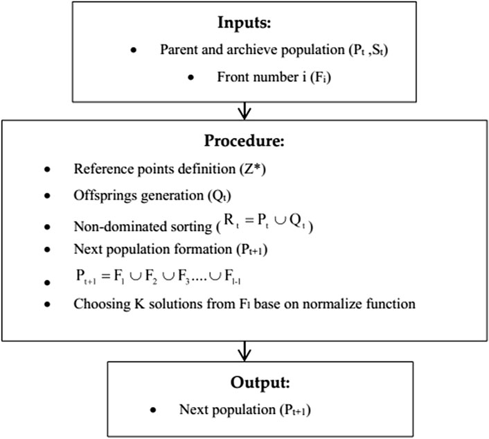
Figure 1. NSGA-III flowchart.

3.3.3 MOSOA

MOSOA is a metaheuristic algorithm in the field of overall optimization that has improved the globally optimum convergence. It is inspired by the foraging behavior of seagulls. It is a relatively new algorithm, but it has been shown to be effective for solving a variety of optimization problems, including multi-objective optimization problems. Its whole detailed process is described in more detail in Pansota et al. (2021).

3.4 Sim&Corrloss clustering method

In this paper, a clustering method called the Sim&Corrloss algorithm is used in scenario analysis to avoid unreliable decision-making. Unreliability results from the interaction between random variables and their correlations. The clustering algorithm used is based on the similarity and dependence of the saved scenarios after their reduction. The clustering method must be designed to preserve the correlation between the random variables. In the Sim&Corrloss clustering method, the objective function is developed based on the correlation loss and similarity functions as Equations 68–70:

$\mathit{max}{\displaystyle \sum _{m=1}^{\stackrel{\sim }{N_l}}}{\displaystyle \sum _{i\in I_m}}\left(Sim\left({\xi }_i-{\xi }_m\right)-\beta Corrloss\left({\xi }_i-{\xi }_m\right)\right)s.t\bigcup _{m=1}^{N_l}={\mathrm{\Omega }}_l,{\displaystyle \sum _{i\in {\mathrm{\Omega }}_l}}{p}_i=1{\mathrm{I}}_m\cap {\mathrm{I}}_{m^{\prime }}=0,\forall m\ne m^{\prime },m,m^{\prime }\in 1,2,\dots ,N_l,(68)$

$sim\left({\xi }_i,{\xi }_j\right)=\frac{1}{d}\left[{\displaystyle \sum _{k=1}^d}\left(1-\frac{p_i{p}_j}{p_i{+p}_j}\right)\frac{\left|{{\xi }_i}^k-,{{\xi }_j}^k\right.}{\left|\max \left\{{{\xi }_l}^k\right\}-\min \left.\left\{{{\xi }_l}^k\right\}\right|+\epsilon \right.}\right],(69)$

$corloss\left({\xi }_i,{\xi }_j\right)={\displaystyle \sum _{i=1}^{d-1}}{\displaystyle \sum _{j=i+1}^d}{\left({\Delta \rho }_{ij}\right)}^2.(70)$

In the Sim&Corrloss clustering algorithm, the parameters are chosen based on a balance between maintaining similarity between the original scenario set and minimizing correlation loss during the scenario reduction process. In this algorithm, the ratio β is crucial as it controls the trade-off between the correlation loss and the similarity during scenario reduction, and the objective is to find an optimal value of β that yields the best performance while ensuring stability in the reduced scenario set. In this paper, β is tested one by one from 0 to 1 with a 0.1 interval through a large number of simulation tests. This method is explained in more detail in Hu and Li (2019). To lessen the scenarios, the average values of solar irradiance, wind speed, and load demand over 24 h are calculated, and then the Sim&Corrloss clustering method is used.

4 Results and discussion

In order to validate the contributions of this work, a test IES was studied, including several electrical power sources, a CHP plant, a P2G unit, two heat boilers, and three storage devices. In this section, simulation is performed to illustrate the validity and effectiveness of our model of operation.

4.1 The test IES

The test IES used to validate the proposed optimal management strategy is shown in Figure 2. All the data used in the study can be found in Yu et al. (2018). The simulation is performed over a period of 1 day, and the results of the energy analysis are obtained in hourly intervals. The parameters of the algorithms are listed in Table 1. The values of the parameters required for the simulation are presented in Tables 2–10. As shown in Figure 2, the test case system contains various energy components, including an electric boiler, a gas boiler transformer, a CHP plant, an ESS, an HSS, a GS, a P2G converter, a wind turbine, an SPV unit, a hot water pipeline, a compressor, and a gas pipeline. Each subsystem in the IES has its own converters with unique energy dispatch coefficients and energy conversion efficiencies. The required parameters of the components are listed in Table 3. In summary, both electric and heat loads are included in the DRP. The maximum generation of the wind turbine is set to 50 MW, and the capacity of the SPV unit is set to 27 MW. Additional data required for these sources can be found in Yu et al. (2018). To demonstrate the validity of the proposed technique, 1,000 scenarios are generated with random variables, which are then reduced to 30 scenarios using a clustering algorithm.

Figure 2

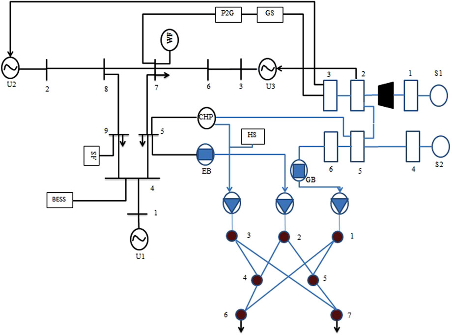
Figure 2. Test case of the IES.

Table 1

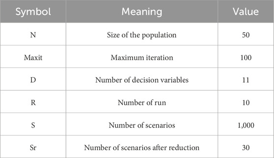
Table 1. Parameters of NSGA-III and MOSOA.

Table 2

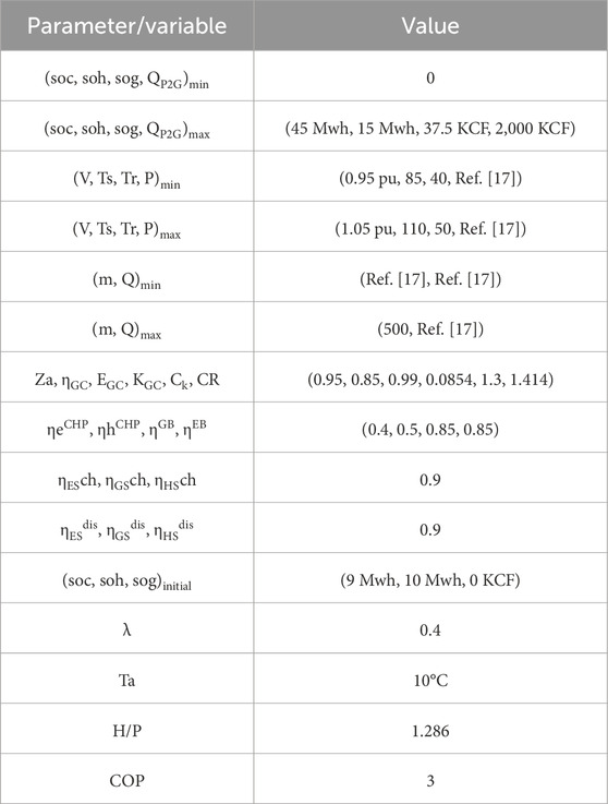
Table 2. Values and limits of variables and parameters in the test IES.

Table 3

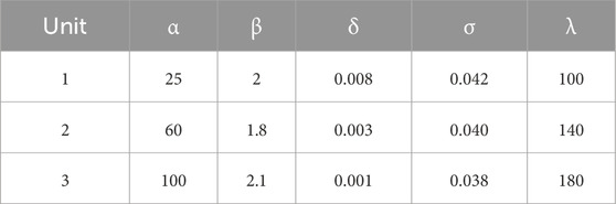
Table 3. Generator cost function parameters and CHP cost function parameters.

Table 4

Table 4. CHP cost function parameters.

Table 5

Table 5. Heat-only cost function parameters.

Table 6

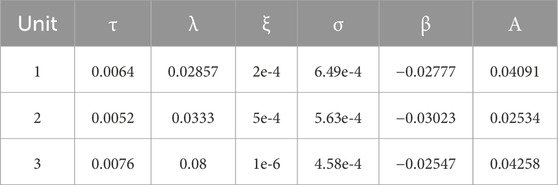
Table 6. Emission cost parameters of the power-only units.

Table 7

Table 7. Emission cost parameters of the CHP.

Table 8

Table 8. Emission cost parameters of the heat-only units.

Table 9

Table 9. Values of the marginal cost of each generating unit and storage.

Table 10

Table 10. Start-up and shut-down cost.

The optimal scheduling of the IES in the most probable scenario, aiming to minimize the total losses and total operating and emission costs, is presented in Figures 3–5. Power generation units such as the SPV unit, wind turbines, and CHP plant are assumed to be capable of injecting both active (P) and reactive (Q) power, and their installation location is considered to be the PQ bus. The optimal Pareto front obtained in the scenario with the highest probability of occurrence is shown in Figure 6, which depicts the total losses and total operating costs of the system over a 24-h period. The statistical analysis of the objective functions defined in the optimization process is presented in Table 11. These results indicate that the changes in the objective functions remain within the specified range when the load demand, wind speed, and solar irradiance change. This suggests that the proposed method can effectively handle changes in input variables and their impact on output variables. Additionally, it emphasizes the importance of considering all aspects of the problem in short-term studies. Finally, the obtained statistical values are compared to the results obtained using MOSOA. The optimal Pareto front presented in Figure 6 shows the compromise point determined using NSGA-III for the optimization problem. The total operating and emission costs are 1.1602 E+05 $, and the total loss value is 0.1188 E+02 MW. The corresponding values for the objective functions obtained using MOSOA are 1.1593 E+05 $ and 0.1189 E+02 MW. When it comes to reducing the loss value for a true operating point, NSGA-III demonstrates superior performance, whereas MOSOA performs better in reducing total costs. As a result, a trade-off must be struck between minimizing loss and minimizing cost in operational optimization.

Figure 3

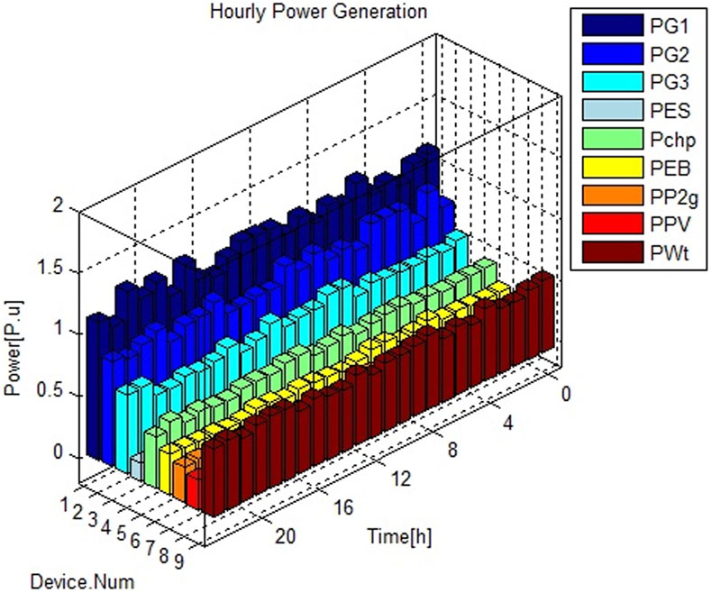
Figure 3. Optimal daily dispatch of the power generation units.

Figure 4

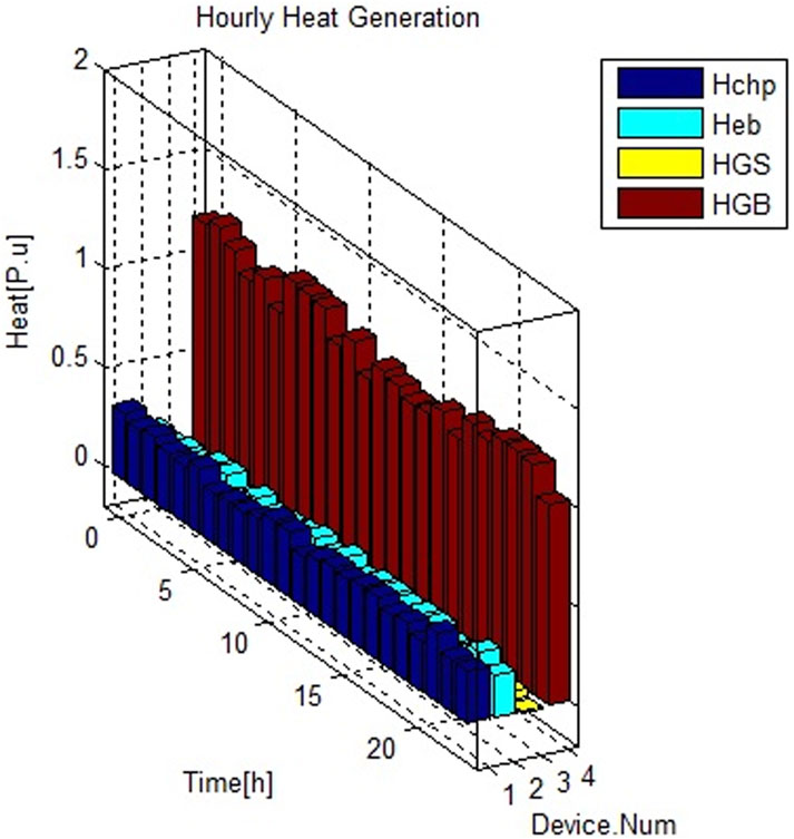
Figure 4. Optimal daily dispatch of the heat generation units.

Figure 5

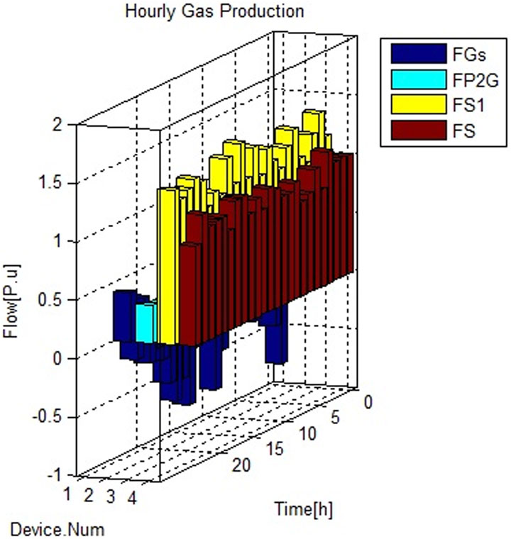
Figure 5. Optimal daily dispatch of the gas generation units.

Figure 6

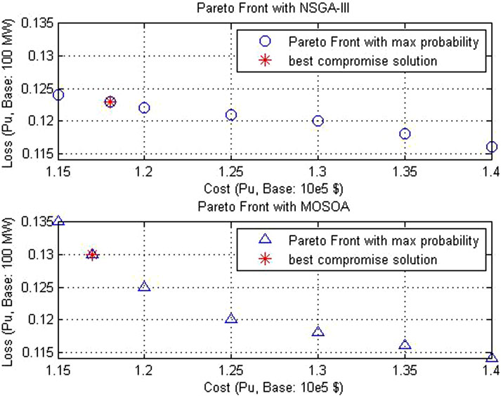
Figure 6. Pareto front obtained through NSGA-III and MOSOA.

Table 11

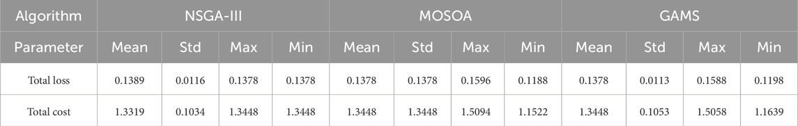
Table 11. Statistical analysis of the objective functions.

During the time intervals [01:00, 07:00] and [21:00, 24:00], the SPV plant does not generate any electricity, and the electricity demand is met by other power sources, whereas the ESS is charged. The CHP plant also supplies electricity during these periods. When the SPV plant generates more electricity, the net consumption of the electric boiler and P2G increases to meet the heat and gas demand. During the periods of low wind power generation, the load on the P2G decreases, but the output of thermal power plants increases. The operational results of the heat generation units and storage device are depicted in Figure 4. As shown, the dispatchable unit’s heat generation increases, whereas the gas boiler’s heat generation decreases. This necessitates an expansion of both gas and electricity generation. Heat storage ensures that the heat surplus or deficit throughout the day is compensated.

The power generated by the RES is proportional to wind speed and solar irradiance, and this is taken into account in the optimization process. However, the charging and discharging of storage devices are generally proportional to energy consumption, considering the type of load in each subsystem. This means that storage devices should be charged when energy consumption is low and discharged when consumption is high. Optimal management is implemented with a DRP for electrical and thermal loads. Load shifting is employed to smooth the load profile.

These figures demonstrate that the integration of renewable energy sources and energy storage enhances system sustainability, resilience, and flexibility to address critical conditions.

As shown in Figure 7, by implementing DRPs and shifting loads to off-peak hours, storage devices are expected to discharge during peak demand periods and charge during off-peak hours. This optimizes storage utilization, reduces load fluctuations, and enhances system robustness.

Figure 7

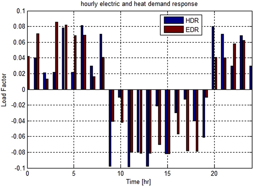
Figure 7. Optimal electrical and heat load factors in the presence of a DRP.

A statistical analysis of the objective functions defined in the optimization process is presented in Table 11. It contains quantitative statistical analysis of the objective functions, total loss and total cost, for the three algorithms: NSGA-III, MOSOA, and GAMS. The headers represent statistical metrics: mean (average value), Std (standard deviation), max (maximum value), and min (minimum value). The associated data entries are the computed values for total loss (in per-unit, Pu, with base 1e5 MW) and total cost (in per-unit, Pu, with base 1e5 $). The minimum and maximum values of the objective functions for total loss and total cost are found to be within the ranges [0.1178–0.1581] and [1.1521–1.5095], respectively. Statistical analysis of the optimization process reveals that the objective functions, total loss and total cost, are constrained within specified ranges. It is important to note that in statistical analysis, the average value represents the central tendency of the data, w the standard deviation quantifies the dispersion of the data around the mean value. Correspondingly, the average values for the loss function and the total cost function are found to be 0.1389 and 1.3319, respectively. The standard deviations for the loss function and the total cost function are 0.0116 and 0.1034, respectively. These results suggest that the changes in the objective functions, namely, total loss and total cost, will be constrained within the specified ranges when the load demand, wind speed, and solar irradiance undergo variations. This indicates the effective capture of input–output relationships by the proposed method. Moreover, the inherent complexity of energy problems underscores the significance of statistical analysis in short-term studies for optimal energy management systems. The obtained statistical values are compared with those obtained via the MOSOA algorithm and GAMS solver.

A comparative analysis was conducted among NSGA-III, MOSOA, and the GAMS solver. The findings clearly indicate that NSGA-III is superior to MOSOA in minimizing the cost function. Conversely, as the cost function decreases, the loss function tends to increase, suggesting a trade-off between these two objectives. However, it is important to note that the performance of both algorithms may vary depending on the specific characteristics of the problem. Table 12 shows this conclusion. As shown in Table 13, in the scenario with the highest probability of occurrence, PAR is decreased by 5.4247% and 0.1691% in the electrical and gas networks, respectively. In the unscheduled operation scenario, where there is no optimization or scheduling, the PAR in both the electric and gas networks is the highest. This indicates greater pressure on the network during peak times, signifying inefficient energy usage and higher operational stress. In comparison, it can be said that with NSGA-III, the PAR decreases in both the electric and gas networks.

Table 12

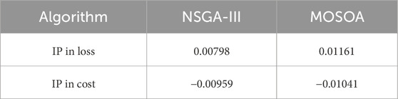
Table 12. Improvement percentage (IP).

Table 13

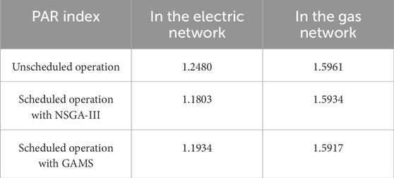
Table 13. PAR index.

In addition, in the energy hub, based on the definition of an index to measure the energy performance of an energy hub, the total energy input is compared to the total energy output. This index is defined as the ratio between the total energy output and the total energy input. It is expressed as an energy efficiency index (EEI), whose higher value indicates higher efficiency and lower total energy loss. This index is evaluated under three operational modes. As shown in Table 14, in the scenario with the highest probability of occurrence, the results indicate that scheduling with both NSGA-III and GAMS algorithms improved the energy efficiency, with NSGA-III showing a more significant improvement.

Table 14

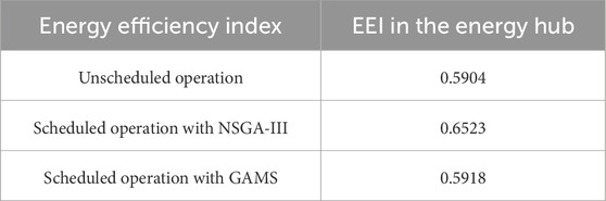
Table 14. EEI.

4.2 Highlighted preferences of the proposed approach

• Most conventional energy management systems (EMSs) do not fully consider the state variables of the three subsystems in the IES. In contrast, the proposed approach comprehensively captures all the state variables based on load flow analysis, heat flow analysis, and gas flow analysis in the EPS, DHS, and NGS, respectively. This enables the optimization of loss function and cost function.

• The IES model in existing studies does not incorporate all the components simultaneously, including CHP, P2G, ESS, HSS, GS, RES, EB, and GS. However, the proposed model integrates these components simultaneously for a more comprehensive and holistic representation of the IES.

• None of the previous studies employed minimization of heat losses and reduction of power losses associated with pressure drop as objective functions.

• Although previous studies focused primarily on electrical load control, the proposed model extends to both electrical and thermal load control. This broader perspective enables more effective optimization of the system’s performance.

• The uncertainty of solar radiation, wind speed, and electric load demand is simultaneously considered in the proposed EMS. This sets it apart from existing studies that only treat these variables individually. The comprehensive treatment of uncertainty enhances the robustness and adaptability of the proposed model to real-world conditions.

• None of the mentioned studies considered the correlation between random variables. The proposed model addresses this gap by employing the Sim&Corrloss clustering method. This clustering method facilitates efficient and reliable optimization, making the proposed approach more robust.

• The optimization problem of EMS is defined as a stochastic multi-objective model, allowing for considering multiple objective functions simultaneously. NSGA-III is employed due to its efficiency and ability to find optimal solutions.

4.3 The limitations of the proposed approach

• The model does not consider the connection to upstream electricity, gas, and heat networks. This simplification was made to focus on the local energy system optimization. However, future research could explore the impact of interactions with larger networks and the potential for energy exchange.

• The scenario tree was not employed to define the 24-h scenarios. Although scenario trees are a powerful tool for modeling uncertainty, their use can lead to a significant increase in computational burden, especially over a 24-h period.

• The convex optimization was not performed. Due to the complexity of the model and the presence of non-linear constraints, direct application of convex optimization was not possible. Future research could explore the use of linear approximation methods to transform the model into a format suitable for convex optimization.

It is important to note that these limitations do not diminish the value of this study but rather highlight potential avenues for future research and the development of more comprehensive models.

5 Conclusion

This paper introduces an optimal energy management approach for an IES based on the NSGA-III algorithm. The proposed approach effectively addresses the challenges posed by uncertainty, renewable energy integration, and cost optimization in power systems. By employing the Sim&Corrloss clustering technique, the computational complexity of the optimization problem is significantly reduced. To manage the impact of parameter uncertainty, a comprehensive range of storage devices is utilized. Moreover, a DRP is implemented to compensate for generation capacity limitations and enhance energy efficiency. The optimization objectives encompass minimizing total losses, emissions, and operating costs. The performance of the proposed approach is evaluated based on its ability to effectively utilize RES units and storage devices, thereby reducing overall losses and operating expenses across all three subsystems. Simulation results are compared with those obtained using the multi-objective simulated annealing (MOSOA) and GAMS solver, demonstrating the superior performance of the proposed approach. Based on the numerical findings obtained from the test system, the following conclusions can be drawn:

• The proposed model provides accurate solutions to the optimization problem, making it an invaluable tool for energy management.

• The proposed optimization technique achieves near-optimal solutions by striking a suitable balance between the conflicting objectives.

• The proposed IES enhances the flexibility of the power system through efficient management of RES and storage resources.

• By converting excess RES energy into converter units, the proposed approach effectively mitigates the impact of RES power constraints and optimizes system performance.

In conclusion, the proposed energy management approach offers a robust and reliable solution for optimizing energy consumption, reducing costs, and enhancing the flexibility of power systems. Its ability to handle uncertainty, integrate RES, and balance multiple objectives makes it a valuable tool for the future of energy management.

Data availability statement

The raw data supporting the conclusions of this article will be made available by the authors, without undue reservation.

Author contributions

HF: writing – original draft and writing – review and editing. NG: conceptualization, methodology, supervision, and writing – review and editing. FS: methodology, supervision, and writing – review and editing.

Funding

The author(s) declare that no financial support was received for the research and/or publication of this article.

Conflict of interest

The authors declare that the research was conducted in the absence of any commercial or financial relationships that could be construed as a potential conflict of interest.

Generative AI statement

The author(s) declare that no Generative AI was used in the creation of this manuscript.

Publisher’s note

All claims expressed in this article are solely those of the authors and do not necessarily represent those of their affiliated organizations, or those of the publisher, the editors and the reviewers. Any product that may be evaluated in this article, or claim that may be made by its manufacturer, is not guaranteed or endorsed by the publisher.

References

Alghamdi, A., Alanazi, M., Alanazi, A., Qasaymeh, Y., Zubair, M., Awan, A. B., et al. (2023). Energy hub optimal scheduling and management in the day-ahead market considering renewable energy sources, CHP, electric vehicles, and storage systems using improved fick’s law algorithm. Appl. Sci. 13, 3526. doi:10.3390/app13063526

CrossRef Full Text | Google Scholar

Bhesdadiya, R. H., Trivedi, I. N., Jangir, P., Jangir, N., and Kumar, A. (2016). An NSGA-III algorithm for solving multi-objective economic/environmental dispatch problem. Cogent Eng. 3, 1269383. doi:10.1080/23311916.2016.1269383

CrossRef Full Text | Google Scholar

Chen, S., and Wang, S. (2020). An optimization method for an integrated energy system scheduling process based on NSGA-II improved by tent mapping chaotic algorithms. Processes 8, 426. doi:10.3390/pr8040426

CrossRef Full Text | Google Scholar

Chen, Y., Zhang, Y., Wang, J., and Lu, Z. (2020). Optimal operation for integrated electricity–heat system with improved heat pump and storage model to enhance local energy utilization. Energies 13, 6729. doi:10.3390/en13246729

CrossRef Full Text | Google Scholar

Darbandi, B., Brockmann, G., Ni, S., and Kriegel, M. (2024). Energy scheduling strategy for energy hubs using reinforcement learning approach. J. Build. Eng. 98, 111030. doi:10.1016/j.jobe.2024.111030

CrossRef Full Text | Google Scholar

Dhiman, G., Singh, K. K., Soni, M., Nagar, A., Dehghani, M., Slowik, A., et al. (2020). MOSOA: a new multi-objective seagull optimization algorithm. Expert Syst. Appl. 143, 114150. doi:10.1016/j.eswa.2020.114150

CrossRef Full Text | Google Scholar

Dong, Q., Sun, Q., Huang, Y., Li, Z., and Cheng, C. (2019). Hybrid possibilistic-probabilistic energy flow assessment for multi-energy carrier systems. IEEE Access 7, 176115–176126. doi:10.1109/access.2019.2943998

CrossRef Full Text | Google Scholar

Duan, J., Liu, F., Yang, Y., and Jin, Z. (2021). Flexible dispatch for integrated power and gas systems considering power-to-gas and demand response. Energies 14, 5554. doi:10.3390/en14175554

CrossRef Full Text | Google Scholar

Ghaffarpour, R. (2020). Stochastic optimization of operation of power to gas included energy hub considering carbon trading, demand response and district heating market. J. Energy Manag. Technol. (JEMT) 4 (3). doi:10.22109/jemt.2020.190206.1183

CrossRef Full Text | Google Scholar

Hu, J., and Li, H. (2019). A new clustering approach for scenario reduction in multi-stochastic variable programming. IEEE Trans. Power Syst. 34 (5), 3813–3825. doi:10.1109/tpwrs.2019.2901545

CrossRef Full Text | Google Scholar

Jiang, T., Deng, H., Bai, L., Zhang, R., and Chen, H. (2018). Optimal energy flow and nodal energy pricing in carbon emission-embedded integrated energy systems. CSEE J. Power Energy Syst. 4 (2), 179–187. doi:10.17775/cseejpes.2018.00030

CrossRef Full Text | Google Scholar

Jin, X., Mua, Y., Jia, H., Wu, J., Xu, X., and Yu, X. (2016). Optimal day ahead scheduling of integrated urban energy systems. Appl. Energy 180, 1–13. doi:10.1016/j.apenergy.2016.07.071

CrossRef Full Text | Google Scholar

Klinkel, K. (2020). Combined simulation of district heating and electrical power networks. Eindhoven, Netherlands: Eindhoven University of Technology.

Google Scholar

Leung, T. (2015). Coupled natural gas and electric power systems. Massachusetts Institute of Technology.

Google Scholar

Li, J., Fang, J., Zeng, Q., and Chen, Z. (2015). Optimal operation of the integrated electrical and heating systems to accommodate the intermittent renewable sources. Appl. Energy 167, 244–254. doi:10.1016/j.apenergy.2015.10.054

CrossRef Full Text | Google Scholar

Li, Q., An, S., and Gedra, T. W. (2003). “Solving natural gas loadflow problems using electric loadflow techniques,” Engineering.

Google Scholar

Li, Y., Wang, C., Li, G., and Chen, C. (2020). Optimal scheduling of integrated demand response-enabled integrated energy systems with uncertain renewable generations: a Stackelberg game approach. Energy Convers. Manag. 235, 113996. doi:10.1016/j.enconman.2021.113996

CrossRef Full Text | Google Scholar

Li, Y., and Zio, E. (2012). Uncertainty analysis of the adequacy assessment model of a distributed generation system. Renew. Energy 41, 235–244. doi:10.1016/j.renene.2011.10.025

CrossRef Full Text | Google Scholar

Liu, X. (2013). Combined analysis of electricity and heat networks. Institute of Energy, Cardiff University.

Google Scholar

Lv, J., Zhang, S., Cheng, H., and Fang, S. (2019). Optimal day ahead operation of user-level integrated energy system considering dynamic behaviour of heat loads and customers' heat satisfaction. IET Smart Grid 2 (3), 320–326. doi:10.1049/iet-stg.2019.0065

CrossRef Full Text | Google Scholar

Naderi, E., Narimani, H., Pourakbari-Kasmaei, M., Cerna, F. V., Marzband, M., and Lehtonen, M. (2021). State-of-the-Art of optimal active and reactive power flow: a comprehensive review from various standpoints. Processes 9, 1319. doi:10.3390/pr9081319

CrossRef Full Text | Google Scholar

Niu, B., et al. (2021). A population-based clustering technique using particle swarm optimization and k-means. Springer Science+Business Media Dordrecht.

Google Scholar

Nojavan, S., Majidi, M., and Zare, K. (2018). Optimal scheduling of heating and power hubs under economic and environment issues in the presence of peak load management. Energy Convers. Manag. 156, 34–44. doi:10.1016/j.enconman.2017.11.007

CrossRef Full Text | Google Scholar

Pansota, M. S., et al. (2021). Scheduling and sizing of campus microgrid considering demand response and economic analysis. Energy, Sustain. Soc.

Google Scholar

Quan, H., Yang, D., Khambadkone, A. M., and Srinivasan, D. (2018). A stochastic power flow study to investigate the effects of renewable energy integration. IEEE, 978-1-5386-4291–7/18/$31.00c.

Google Scholar

Sadeghi, A., Ahmadian, A., Diabat, A., and Elkamel, A. (2024). Modeling energy management of an energy hub with hybrid energy storage systems for a smart island considering water–electricity nexus. Int. J. Hydrogen Energy 71, 600–616. doi:10.1016/j.ijhydene.2024.05.250

CrossRef Full Text | Google Scholar

Shaabani, Y. A., Seifi, A. R., and Kouhanjani, M. J. (2017). Stochastic Multi-objective optimization of combined heat and power economic/emission dispatch. Energy 141, 1892–1904. doi:10.1016/j.energy.2017.11.124

CrossRef Full Text | Google Scholar

Shahrabi, H., Hakimi, S. M., Hasankhani, A., Derakhshan, G., and Abdi, B. (2021). Developing optimal energy management of energy hub in the presence of stochastic renewable energy resources. Sustain. Energy, Grids Netw. 26, 100428. doi:10.1016/j.segan.2020.100428

CrossRef Full Text | Google Scholar

Shekari, T., Gholami, A., and Aminifar, F. (2019). Optimal energy management in multi-carrier microgrids: an MILP approach. Clean. Energy 7 (4), 876–886. doi:10.1007/s40565-019-0509-6

CrossRef Full Text | Google Scholar

Thang, V. V., Zhang, Y., Ha, T., and Liu, S. (2018). Optimal operation of energy hub in competitive electricity market considering uncertainties. Int. J. Energy Environ. Eng. 9, 351–362. doi:10.1007/s40095-018-0274-8

CrossRef Full Text | Google Scholar

Turk, A., Zeng, A., Wu, Q., Nielsen, Q., and Hejde, A. (2020). Optimal operation of integrated electrical, district heating and natural gas system in wind dominated power system. Int. J. Smart Grid Clean Energy 9 (2), 237–246. doi:10.12720/sgce.9.2.237-246

CrossRef Full Text | Google Scholar

Wei, W., and Wang, J. (2020). Modeling and optimization of interdependent energy infrastructures. Switzerland: Springer Nature. 978-3-030-25958-7.

Google Scholar

Woldeyohannes, A. D., and Abd Majid, M. A. (2021). Simulation model for natural gas transmission pipeline network system. Simul. Model. Pract. Theory 19, 196–212. doi:10.1016/j.simpat.2010.06.006

CrossRef Full Text | Google Scholar

Wu, H., Li, H., and Gu, X. (2020). Optimal energy management for microgrids considering uncertainties in renewable energy generation and load demand. Processes 8, 1086. doi:10.3390/pr8091086

CrossRef Full Text | Google Scholar

Yadollahi, G., Gharibi, R., Dashti, R., and Torabi Jahromi, A. (2024). Optimal energy management of energy hub: a reinforcement learning approach. Sustain. Cities Soc. 102, 105179. doi:10.1016/j.scs.2024.105179

CrossRef Full Text | Google Scholar

Yu, J., Guo, L., Ma, M., Kamel, S., Li, W., and Song, X. (2018). Risk assessment of integrated electrical, natural gas and district heating systems considering solar thermal CHP plants and electric boilers. Electr. Power Energy Syst. 103, 277–287. doi:10.1016/j.ijepes.2018.06.009

CrossRef Full Text | Google Scholar

Yuan, Z., Alizadeh, A., Nojavan, S., and Jermsittiparsert, K. (2020). RETRACTED: probabilistic scheduling of power-to-gas storage system in renewable energy hub integrated with demand response program. J. Energy Storage 29, 101393. doi:10.1016/j.est.2020.101393

CrossRef Full Text | Google Scholar

Zhang, H., Wang, G.-G., Dong, J., and Gandomi, A. H. (2021). Improved NSGA-III with second-order difference random strategy for dynamic multi-objective optimization. Processes 9, 911. doi:10.3390/pr9060911

CrossRef Full Text | Google Scholar

Zhong, Y., Xie, D., Zhai, S., and Sun, Y. (2018). Day ahead hierarchical steady state optimal operation for integrated energy system based on energy hub. Energies 11, 2765. doi:10.3390/en11102765

CrossRef Full Text | Google Scholar