Future marine biofuels in the port of Seattle region

Marine transportation, a vital global sector, emits 3% of global annual greenhouse gas emissions, which are predicted to increase in the future. Marine biofuels derived from biomass or waste sources like wood residue, waste oil and municipal solid waste can be used for decarbonization. However, limited studies have explored if sufficient marine biofuels could be produced and supplied to major regional ports given feedstock, supply chain and technological constraints. We fill this gap by evaluating the feasibility of supplying marine biofuels to the Port of Seattle. The Regional Bio-Economy Model (RBEM) and the Freight and Fuel Transportation Optimization Tool (FTOT) are used to build scenarios for simulating marine biofuel production in the Port region. We harmonized technoeconomic assumptions for RBEM and FTOT, input FTOT feedstock utilization and routing outputs into RBEM, and modelled conversion, feedstock, and policy scenario variations in RBEM. In RBEM, overall biofuel production was constrained primarily by the biofuel cost, and then by feedstock availability. Providing policy incentives and reducing permitting time frames alleviated these constraints and spurred the buildout of a robust industry through industrial learning dynamics in the initial years. With these measures in place, the RBEM results show that 100% of fuel demand at the Port can be supplied by biofuels with policy incentives and suitable technoeconomic conditions, but the addition of transportation cost considerations using FTOT led to 27.8% of demand being able to be met by biofuels at reasonable fuel delivery cost.

1 Introduction

Marine transportation plays a vital role in the global economy, accounting for more than 80% of global trade by volume (UNCTAD, 2012). The shipping industry is also responsible for approximately 3% of total global greenhouse gas (GHG) emissions, and its emissions are projected to increase between 50% and 250% by 2050 if no action to decarbonize marine fuels is taken (IRENA, 2021). One approach to reduce the contribution of maritime emissions is to shift toward sustainable marine fuels, including biofuels. Several entities have set targets for decarbonizing the shipping industry, which will likely drive the adoption of marine biofuels. For instance, the International Maritime Organization (IMO) has set a target of reducing the shipping industry’s GHG emissions by at least 80% by 2040 compared to 2008 emissions and for net zero carbon emissions “by or around, i.e., close to” 2050 (IMO Marine Environment Protection Committee, 2023). The European Union (EU) has followed suit, setting the same target as the IMO (European Commission, 2023; Saul and Abnett, 2021).

Marine diesel engines, which are more efficient than gasoline engines, are used to power marine transportation. These engines primarily use marine gas oil, marine diesel oil, intermediate fuel oil, marine fuel oil and heavy fuel oil. These marine fuels have a higher density and flashpoint and a lower cetane number than conventional automotive diesel (Mohd Noor et al., 2018). Biofuels have fuel characteristics and combustion properties very close to heavy fuel or marine diesel oils and have been identified as promising solutions for meeting emissions targets by the IMO (Kesieme et al., 2019). Marine biofuels can be derived from different biomass sources—such as wood waste, waste oils, and other organic materials—and have the potential to reduce GHG emissions by up to 90% compared to fossil fuels (Simonsen et al., 2021). The market penetration of marine biofuels is currently low, accounting for less than 1% of total marine fuel consumption (Kesieme et al., 2019). However, several pilot projects, case studies, and other deployment projects have been initiated to test the performance and feasibility of marine biofuels in real-world settings.

In 2020, bp and Maersk Tankers conducted successful trials of B30 (30% biodiesel) marine fuel using a combination of used cooking oil and other waste materials as feedstocks. Similarly, ExxonMobil completed two commercial deliveries in 2022, using a B25 blend made from vegetable oils (ExxonMobil, 2022). Exxon estimates the blend could reduce GHG emissions by up to 40% compared to conventional marine fuels (ExxonMobil, 2024). French container ship company CMA CGM has also conducted several successful biofuel trials and had set a goal of replacing 10% of total fuel usage with alternative fuels in 2023 (CMA CGM 2022a; 2022b).

In addition to established biofuels that provide drop-in replacements for diesel or other petroleum-based fuels, other advanced marine fuels such as hydrogen, ammonia, and methanol are being developed and tested but face challenges related to infrastructure investment, competition, safety and handling, and cost competitiveness.

Commercial ship owners are investing in vessels that are technologically prepared to burn alternative fuels. As of 2022, 6.0% of the fleet on the water and 48.8% of the orderbook in tonnage terms could use alternative fuels for propulsion. A record 55% of newbuild orders by tonnage were for alternative fuel vessels (Ovcina Mandra, 2024). However, large vessels have long lifespans, and overall fleet turnover is likely to take decades.

The wider uptake of near-term alternative fuels in the sector is likely to depend on several factors, including policies and regulations, carbon pricing, and new business models focused on low carbon footprint as part of the transport service (Hsieh and Felby 2017; Simonsen et al., 2021).

Recent studies suggest the market penetration of marine biofuels could increase significantly in the coming years and biofuels could supply 15%–20% of marine fuel demand by 2050 (Simonsen et al., 2021; Tan et al., 2021a) with particular opportunities for biofuel production from waste and residues (Tan et al., 2021a). The World Bioenergy Association has also projected significant growth in the marine biofuel market, with a potential market share of up to 5% or 5.2 billion gallons of biofuel by 2030 (Tan et al., 2021b).

Though there are numerous studies on marine fuel options, few explore how alternative marine fuels could be produced and supplied to major regional ports. Currently, there is one study known to the authors providing region-specific supply chain analysis for marine biofuels (Gartland and Pruyn, 2022), which focuses on marine biofuel supply in the EU produced from five feedstocks—agricultural residues, forestry residues, livestock residues, biowaste, and sewage—via three conversion pathways: anaerobic digestion, pyrolysis/hydrolysis, and gasification. The study found the available supply of biomass in the EU is sufficient to meet shipping demand in the foreseeable future. The largest impediment to the adoption of these fuels is the available refining potential in Europe (Gartland and Pruyn, 2022). Outside the EU, no other regional analysis has been conducted.

The objective of this study is to develop a framework to explore the potential for marine biofuels to fulfill regional fuel demand using data on existing potential feedstocks, optimized transportation routes, techno-economics of conversion pathways, policy and economic drivers, and fuel markets to simulate the production and growth of the regional marine biofuels industry. The analytical framework for this analysis leverages the complementarity of two models—the Regional Bio-Economy Model (RBEM) (Inman et al., 2023) and the Freight and Fuel Transportation Optimization Tool (Volpe National Transportation Systems Center 2024). This framework is applied to explore options to meet marine fuel demand with regionally produced, waste-based alternative fuels for the Port of Seattle in the State of Washington based on projected industry development and maturation and geospatial options for the delivery of feedstocks and fuels. The approach outlined herein not only elucidates the potential opportunities for marine biofuels in the Seattle region but demonstrates an analytical approach that can be applied to other regions and fuel production pathways and supply chains.

2 Methods

2.1 Marine biofuels supply chain structure

Delivery of marine biofuels to a port is preceded by a multi-step upstream supply chain (see Figure 1). Waste and woody feedstocks—which we considered in this study—are collected and transported to a biorefinery, where they are processed into biofuels. These biofuels may then be further transported to a blending terminal, where they are (or can be) blended with petroleum fuels before being available for bunkering (refueling) at a port. In this study, we answer key questions about the development of the biofuels industry around the Port of Seattle: Given economic constraints of transportation and the techno-economics of conversion pathways, how much feedstock is viable for marine biofuel production and where are the optimal biorefinery locations? How much biofuel relative to the demand at the port can be produced using the viable feedstock and refinery capacities in the region? How do these geospatial and technology constraints affect the growth of the biofuels industry in the region? Can policies and investments spur biofuels production and technological development through 2040 in the Pacific Northwest (PNW)? Both FTOT and RBEM were leveraged in this analysis to answer these questions.

Figure 1

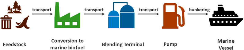
Figure 1. The marine biofuel supply chain.

2.2 Freight and fuel transportation optimization tool

The Freight and Fuel Transportation Optimization Tool is a supply-chain-focused transportation model developed by the Volpe National Transportation Systems Center in Cambridge, MA in support of the Federal Aviation Administration, Office of Naval Research, and Department of Energy. It uses mixed integer linear programming to optimize the transportation of raw and processed materials in a supply chain over a multimodal transportation network to maximize delivery while minimizing transportation costs and/or CO₂ emissions. FTOT uses a geographic information system network that is translated into Python for optimization and analysis. As a geospatially explicit model, FTOT is inherently focused on commodity flows in the region of interest. The user defines a set of origins and production amounts, destinations and demand amounts, and, if desired, definitions for intermediate processing facilities and their size, input/output relationships (i.e., conversion efficiency and product slate determining outputs from processing facilities), and cost to build (if not already built). FTOT attaches these facility locations to the transportation network and uses cost and/or emissions along with various adjustable factors related to routing decisions (e.g., weightings to encourage flows on larger/higher-speed roadways rather than smaller roads) and supply-chain-specific considerations (e.g., facility size, conversion efficiency, product slates) to deliver materials through the supply chain—resulting in delivery of the final product to demand centers. The optimal solution provides transportation routing and flows over the network for the scenario as well as associated transport cost, emissions, vehicle miles traveled (VMT), and miles of network used by commodity and mode. FTOT is a publicly available, open-source tool with extensive documentation, instructional videos, and other materials (Volpe National Transportation Systems Center, 2024).

In this analysis, feedstock locations and projected amounts, conversion techno-economics for marine biofuel pathways, locations of existing refineries and blending terminals in the region, and projected fuel demand at the Port of Seattle were used as inputs for FTOT. FTOT’s default multimodal contiguous U.S. network—consisting of roadways, railroads, inland and costal waterways, and crude and product pipelines—was used for the analysis. FTOT was run optimizing on transportation costs only.

2.3 Regional bio-economy model

The Regional Bio-Economy Model is a system dynamics (SD) model developed at NREL (Inman et al., 2023). System dynamics is an established modeling methodology (Sterman et al., 2003) that demonstrates the potential interactions within and among systems as they evolve over time using stocks and flows and how these interactions could change with different external factors (e.g., policy). Stocks represent accumulations such as inventories or production capacities. Flows represent activities—such as producing, consuming, or investing—that cause accumulations to grow or decline over time. The RBEM model was created using Stella software (IRENA, 2021), which allows the building of system dynamics models that can incorporate feedback loops, time delays, and other important features of complex systems.

RBEM is organized into a set of six modules, each of which houses a component of the feedstock-to-biofuels system. For this analysis, we modified the model to represent feedstocks and conversion pathways that are being considered for marine biofuel. The model contains separate modules for fats, oils, and greases (FOG); municipal solid waste (MSW); sludge; and woody feedstock sources that represent feedstock availability, transport, and prices. A single conversion module is used to represent five distinct conversion processes (Figure 2). It simulates the potential buildout of biorefineries based on feedstock availability and price, conversion pathway techno-economic data, policy incentives, and a net-present-value-based investment logic. An end-use module tracks the disposition of fuels; it represents the current conventional fuels markets and is used by the conversion module to evaluate competition between conventional fuels and biofuels. The model simulation runs from 2020 through 2040. More information on the model can be found in Inman et al. (2023).

Figure 2

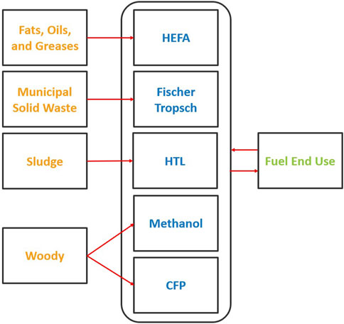
Figure 2. Structure of RBEM. The bold black lines represent modules in the model.

RBEM renders itself to scenario and sensitivity analysis to explore dynamics of the bioeconomy. In this analysis, local feedstock availability and pricing in PNW, conversion techno-economics for marine biofuel pathways, industrial learning, policy inputs, and permitting time frames were used as inputs for RBEM to simulate potential regional industry development to supply marine biofuels to the Port of Seattle.

2.4 Coordinated analysis using FTOT and RBEM

RBEM and FTOT are complementary to one another: FTOT focuses on identifying optimized supply chain transport routes for alternative fuels and can help assess likely transport costs and emissions whereas RBEM provides a view of the biofuel industry development trajectory and impacts of policy. In this analysis, the two models leveraged some of the same data inputs regarding the techno-economics of conversion pathways (e.g., processing facility capacity, capital expenditure, operating expenditure, and revenue streams), per-ton-mile transport costs for feedstock and product, and fuel slates. Feedstock availability within “near,” “medium,” and “far” distance categorizations from optimally located biorefineries calculated from FTOT-generated results, along with transportation distances for feedstock and fuels, were fed into RBEM to align the two models (Figure 3).

Figure 3

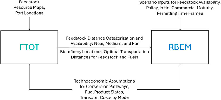
Figure 3. Data flow for coordinated FTOT and RBEM analysis.

2.5 Study overview

This study focused on the potential of biofuel supply chains in the PNW to supply marine fuel demand at the Port of Seattle. A total of 307 million diesel gallon equivalents (DGE) of marine fuel was projected as potential demand in 2040 at the port based on analysis of historical oil transactions from January 2007 to December 2019 for bunker oil, diesel, and other marine fuels (State of Washington, 2021). Because there was no strong trend toward growth or decline in fuel transfers at the Port of Seattle over this time (Figure 4), the average annual fuel demand from 2007 to 2019 was used to project the fuel demand in 2040.

Figure 4

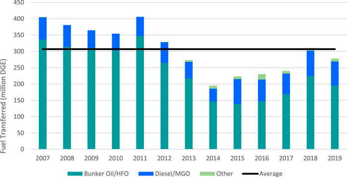
Figure 4. Historical data and average annual fuel demand at the Port of Seattle. For this study, the average value (307,013,838 DGE) was used as the demand value for 2040 at the Port of Seattle. HFO, heavy fuel oil; MGO, marine gasoil.

Given economic and environmental benefits of using waste-based biofuels, the scenarios focused on existing wastes that could be leveraged as biofuel feedstocks in the region: FOG, MSW, sewage sludge, and woody forest and mill residues. These were assumed to be processed using hydroprocessed esters and fatty acids (HEFA) conversion, Fischer-Tropsch (FT) gasification and biorefinery processing, hydrothermal liquefaction (HTL) with mild hydrotreating and blending of biocrude, and coprocessing in existing refining facilities with catalytic fast pyrolysis (CFP), or methanol production, respectively. The pathways selected were chosen due to their relative technological maturity, with one pathway selected per waste feedstock besides the choice between CFP and methanol for wood residues. Other waste-based biofuels pathways were outside the scope of this analysis. Table 1 shows the pathways considered in this study along with regional feedstock descriptions. Pathways 1 through 4b were considered in RBEM whereas FTOT also analyzed an additional Pathway 4c. This additional pathway models CFP from Pathway 4a and methanolization from Pathway 4b together in competition for the wood residues feedstock. The Supplementary Material (SI) includes detailed information on feedstock sourcing and prices (Supplementary Table S4), techno-economic information for conversion processes (Supplementary Table S1), and biorefinery product yields (Supplementary Table S2).

Table 1

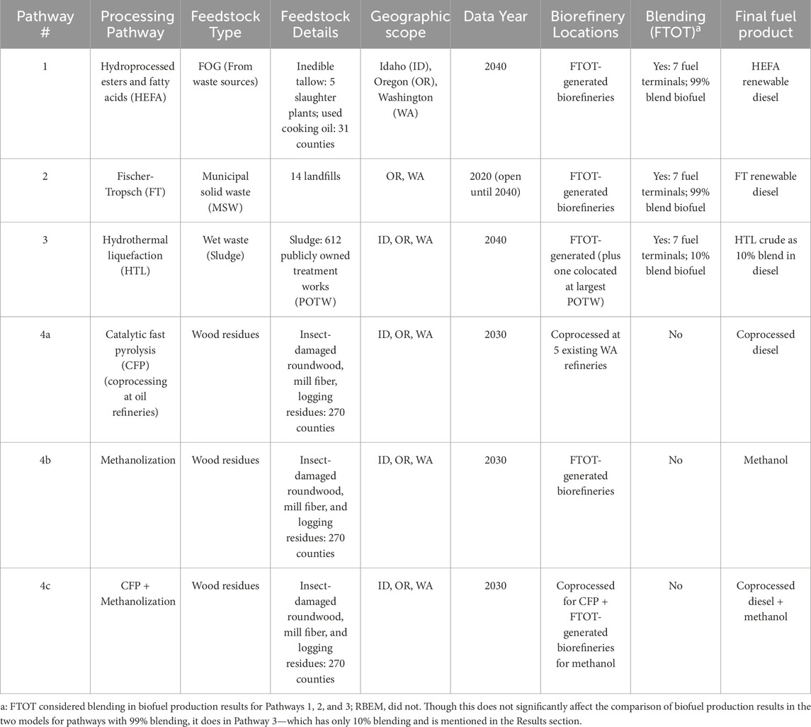
Table 1. Feedstock descriptions and sourcing and associated conversion pathways.

2.6 Scenario analysis

2.6.1 Analysis in FTOT

Each fuel pathway was modeled separately in FTOT to determine a potential fuel supply chain for each feedstock source, optimizing for fuel delivery to the Port of Seattle while minimizing transportation costs and other supply chain costs (e.g., construction of new biorefineries or coprocessing facilities). For Pathways 1 (FOG to HEFA), 2 (MSW to FT), 3 (sludge to HTL), and 4b (wood residues to methanol), FTOT was set up to generate potential biorefinery locations for processing feedstock to fuel based on feedstock locations and amounts, transport cost, and biorefinery capacity and capital cost. For Pathway 3 (sludge to HTL), a potential biorefinery location was also preselected to be co-located with the largest of the publicly owned treatment works (POTW), since this facility has a sludge capacity greater than 110 dry tons per day, an amount economical to support an HTL plant, and as the cost of transporting wet sludge is high (Milbrandt and Badgett, 2024; Snowden-Swan et al., 2017). For Pathway 4a (wood residues to CFP), coprocessing of wood residues was completed at existing refineries in Washington. An additional scenario (Pathway 4c) combined wood residue conversion via CFP and methanolization options into a single scenario to identify which process would be selected if competing against one another for the same feedstock from a transportation cost perspective. Each pathway also includes a maximum feedstock transport distance to account for real-world limitations on the distance feedstock is transported before it is processed into fuel.

For Pathways 1, 2, and 3, FTOT modeled a blending step in the fuel supply chain prior to delivery to the Port of Seattle to reflect policy conditions for biofuels (e.g., blending credits) as well as potential to avoid the cost of upgrading of HTL biocrude by blending directly with diesel at a lower percentage. Therefore, Pathways 1 and 2 produce renewable diesel, which is blended in a 99-to-1 ratio with petroleum-based diesel to provide the port with 99% bio-based fuel. Pathway 3 produces HTL biocrude, which is blended into diesel at a 10-to-90 ratio, so the fuel provided to the port is only 10% biofuel. A 10% blend was chosen for HTL because the water and total acid number (TAN) specifications required make upgrading via hydrotreating an expensive option (Tan and Kaul, 2023). The SI includes detailed schematics for each pathway modeled in FTOT with relevant facility and supply chain data (Supplementary Figures S1 through S5).

Based on the potential facility locations and feedstock availability, FTOT computed a cost-optimized routing solution for transporting feedstock to a subset of candidate biorefineries or coprocessing locations and transporting fuel products from refineries to the blender (when included) and port for each pathway scenario.

Fuel delivery within FTOT is driven by an adjustable parameter called the unmet demand penalty, which penalizes the failure to satisfy fuel demand at the end destination—in this case, the Port of Seattle. This parameter is weighed against the cost of transport and facility build cost and provides a mechanism to tune the model to produce reasonable fuel processing and delivery costs. For each pathway, sensitivity analysis was performed on the unmet demand penalty to find the right balance of feedstock use and demand fulfillment at minimal transport cost to achieve a cost of transport per gallon of delivered biofuel within a realistic range ($0.05 to $0.20) whenever possible.

2.6.2 Processing of FTOT outputs into RBEM inputs

The FTOT solutions were used to generate a list of optimal and nonoptimal combinations of feedstock sources, transportation distances from feedstock sources to a biorefinery or existing refinery, and the quantity of feedstock transported. These outputs were processed to place feedstock production in three distance categories (near, medium, and far, defined in the next paragraph) and passed to RBEM, which represents transport costs categorically and applies an average transport cost for each category. The FTOT outputs thus informed the quantity of feedstock available in RBEM along with the average feedstock transport distance for each of the three categories and the mode used to transport feedstock and product in the routing solution.

FTOT generates an optimal solution for the scenario and utilizes the subset of feedstock sources that contribute to the least-cost outcome. However, other feedstock sources are not necessarily unrealistic. Because RBEM is an SD model that performs a higher-level analysis at the economy wide level, it was allowed to access all available feedstock, even if not used in the FTOT optimal solution. Feedstock was thus placed in the near, medium, and far categories in RBEM based on the percentage of total available feedstock from the PNW region used by FTOT. For MSW and FOG, more than 50% of available feedstock was used in the optimal FTOT solutions. The feedstock quantities and transport distances of optimal locations of MSW and FOG were divided into two groups using a weighted average to inform the near and medium group distances in RBEM. The nonoptimal feedstock locations and associated quantities were used for the far group. Thus, RBEM used feedstock from all locations present in the FTOT scenario, whereas FTOT used feedstock only from the optimal FTOT solution to compute results. Consequently, all available MSW and 68% of available FOG was used in the RBEM inputs in the near, medium, and far groups. For woody biomass, less than 50% of feedstock was used in the optimal FTOT solution, and thus the optimal solution was used for near RBEM inputs. The nonoptimal feedstock locations and associated quantities were divided into two groups using the weighted average to create the medium and far group distances for RBEM; 31% and 14% of available woody feedstock were used for the RBEM inputs in the methanol and CFP scenarios, respectively. For sludge, FTOT co-located all processing at the POTW. The feedstock quantities in the optimal solution were used to create the near group. The feedstock quantities associated with the nonoptimal feedstock locations were used to create the far group. No medium group was created, and all feedstock transport distances were zero because biorefineries were co-located. A total of 40% of available sludge feedstock was used for the RBEM inputs. Table 2 summarizes the translation of feedstock availability and distance from FTOT outputs to RBEM inputs.

Table 2

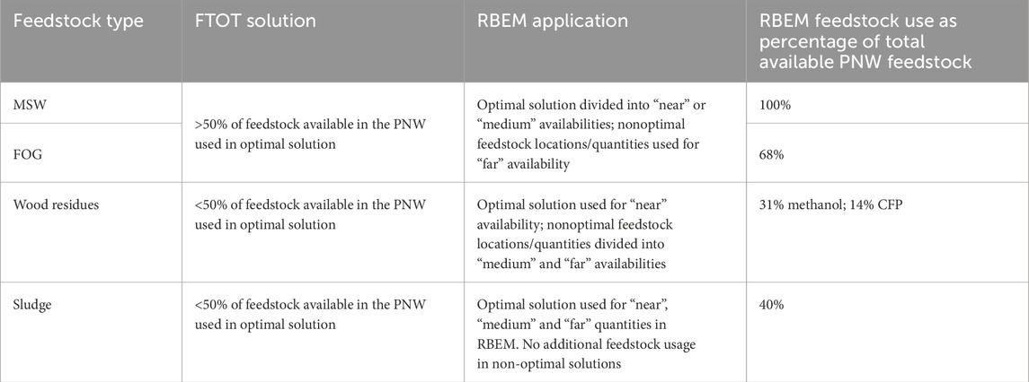
Table 2. Feedstock differentiation in FTOT and RBEM.

The FTOT outputs for the transport of fuel products informed the product transportation distances in RBEM. The weighted-average fuel product transportation distances for each conversion technology were used as the input fuel product transportation distance in RBEM. Finally, FTOT outputs distinguish between modes of transport (e.g., road, rail, or pipeline). The weighted-average travel distance for each feedstock by mode was used to create an overall percent of travel mode for each feedstock and fuel product in RBEM. These percentages were used as inputs in RBEM, with associated costs for each travel mode that aligned with the costs used in FTOT.

2.6.3 Analysis in RBEM

RBEM defines vignettes (a characteristic of the model that can be varied) and variations (options for varying the vignettes) to explore the dynamics of fuel economy. In this study, RBEM vignettes were used to analyze the effect of feedstock availability, policy incentives, permitting time frames, and commercial maturities of conversion pathways at the beginning of the simulation period. In addition, a vignette was created to toggle between the CFP and methanolization pathways because only one of these pathways can use the wood residue feedstock at a time.

Scenarios in RBEM were created using all combinations of possible variation values for each vignette. Table 3 describes the vignettes and variations used in RBEM, whether the vignette is based on FTOT inputs, and whether the variation is a baseline case defined for the analysis.

Table 3

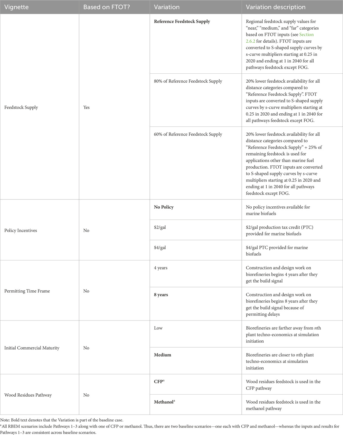
Table 3. Vignettes and variations used in RBEM.

3 Results and discussion

FTOT provides results about the transport costs and modes, amount of used feedstock, biorefineries built, and the amount of biofuel produced.

Table 4 shows the full set of FTOT model results. Transport costs range from $0.16 to $0.65 per DGE of delivered biofuel. The low end of the transport costs range is associated with Pathway 4b (wood residues to methanol), but similar costs are found for Pathway 2 (MSW to FT) and Pathway 3 (sludge to HTL) as well. The high end of the transport costs range is associated with Pathway 1 (FOG to HEFA) and can be attributed to lack of feedstock availability. To satisfy the minimum operating requirements of the HEFA biorefinery, almost all FOG available in PNW is transported to one central location, resulting in high transport costs. Even so, this still leads to an effective minimum turndown (output relative to biorefinery capacity) of 33% at the biorefinery.

Table 4

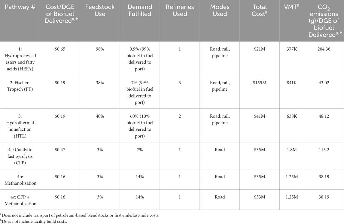
Table 4. Summary table of FTOT model results by pathway to meet projected 2040 demand of 307 million DGE at the Port of Seattle.

Projected fuel demand in 2040 met at the port by individual fuel pathways ranges from 0.9% for Pathway 1 to 60% for Pathway 3, though because of the blending specifications of Pathway 3, only 10% of that delivered fuel is bio-based. Pathways 2, 4a, and 4b—which provide a higher proportion of biofuel to the port—can meet 7%, 7%, and 14% of projected demand, respectively.

RBEM simulations incorporate identical technoeconomic assumptions as FTOT. In addition, they incorporate feedstock availability and transportation costs from FTOT model runs. RBEM simulations incorporate one-to-one mappings of feedstock to conversion pathways, using separate simulations to map woody feedstocks to CFP or to methanol (unlike pathway 4c in FTOT).

Analyses conducted using RBEM in this study highlight how biofuels could be deployed in the PNW region based on feedstock availability, potential policy, techno-economics, and permitting timeframes. Although model outputs may highlight specific quantities, the primary use of the model lies in scenario analysis and comparison of the magnitude and timing of how the industry evolves given differing assumptions and policy scenarios. The baseline scenarios assume feedstock supply as calculated from FTOT results, an 8-year permitting time frame for biorefineries, a medium level of initial commercial maturities for conversion pathways, and no policy incentives. Because wood residues can be used by either CFP or methanolization pathways, two baseline scenarios are shown in each results figure where all results other than those for CFP and methanolization stay constant.

Figure 5 presents RBEM results for the baseline scenarios, along with all variations for the feedstock supply, policy incentive, and wood residues pathway vignettes. Total production from four pathways—each denoted by a color—is summed to compare to the demand at the Port of Seattle on a DGE basis. As seen in comparing the left and right sets of results, whether biofuels produced using feedstocks in PNW can satisfy demand at the port depends on whether wood residues are being routed to CFP or methanol. When wood residues are routed to CFP, the baseline scenario (top left graph in Figure 4) does not reach a production level that meets the Port of Seattle fuel demand in 2040; when they are routed to methanol, the baseline scenario production exceeds the Port of Seattle fuel demand, with the methanol pathway contributing to 95% of fuel production. The following sections explore the FTOT feedstock use, transport, and conversion and RBEM biofuel production results for individual conversion pathways. Later, biofuel production results are analyzed on a regional scale to compare with port demand.

Figure 5

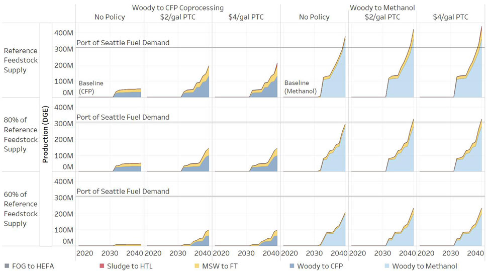
Figure 5. Biofuel production for different pathways, from 2020 to 2040, given differing assumptions on feedstock availability and policy. Reference line shows projected 2040 demand of 307 million DGE at the Port of Seattle.

3.1 Pathway 1: hydroprocessed esters and fatty acids processing of lipids

Results from FTOT show the HEFA pathway is constrained primarily by regional feedstock availability. Even though the feedstock has more flexibility in transport (e.g., no maximum transport distance constraint), absolute feedstock availability is sufficient for input to only one biorefinery and even then, only when the biorefinery is allowed to operate below 50% of maximum capacity. Therefore, though 98% of available feedstock is used, only 0.9% of fuel demand is met. In the FTOT sensitivity analysis around the unmet demand penalty parameter, only one scenario led to any fuel delivered to the Port of Seattle. That scenario sourced feedstock across all three states in PNW and located the biorefinery at a “centralized” location in eastern Washington state. The solution is inelastic to any additional incentive to meet port demand; the minimum operating capacity of the biorefinery is a hard cutoff and operating near that minimum level leads to a solution with high transport cost of delivered biofuel of $0.65/DGE. In RBEM, no HEFA facilities are built in the baseline scenario—this is because the minimum fuel selling price (MFSP) of HEFA is higher than expected returns. When policy incentives of $2/gal or $4/gal are provided, the available feedstock can support only one HEFA plant through 2040, keeping the production lower than 2 million DGE and meeting 0.6% of the port demand.

3.2 Pathway 2: Fischer-Tropsch processing of municipal solid waste

In FTOT results, 38% of MSW feedstock in PNW was used to meet 7% of fuel demand with a fuel that is 99% bio-based. This pathway has relatively few feedstock locations with a large amount of material available at each site. As a result, the FTOT optimal result uses biorefineries—each operating at maximum capacity—essentially co-located at the three landfills from which it is cheapest to transport to the Port of Seattle. FT renewable diesel is transported by rail from northern Oregon landfills to a blending facility near the port. Sensitivity testing in FTOT shows increasing the transportation incentive through the unmet demand penalty parameter leads to five more landfills along the I-5 corridor being used for feedstock, though at significant cost (raising the transport cost per DGE of delivered biofuel from $0.19 to $0.53).

In RBEM, scenarios were run with feedstock supply based on FTOT inputs (in this case, 38% MSW feedstock from PNW; see Section 1.1 for details), with additional variations of 80% and 60% of the baseline feedstock supply to evaluate the sensitivity of FT production to feedstock availability. FT from MSW is produced in the baseline RBEM scenario (Figure 5) because FT is a commercially available technology and MSW is a low-cost feedstock compared to other feedstocks in this analysis. FT production was found to be restricted by feedstock availability especially when a policy to incentivize production is implemented. MSW to FT production is about 18 million DGE in 2040 in the baseline case (5.9% of port fuel demand) and about 61 million DGE (19.9% of port fuel demand) when $2/gal and $4/gal policy incentives are provided. When the availability of feedstock is reduced to 80% or 60% with policy incentives present, MSW to FT production in 2040 increases only to 45 and 35 million DGE, respectively, because not enough feedstock is available to construct more than seven FT plants through 2040.

3.3 Pathway 3: hydrothermal liquefaction processing of sewage sludge

In FTOT results, 40% of feedstock is used, meeting 60% of fuel demand but with a fuel that is only 10% bio-based. HTL crude is not an upgraded fuel and is thus limited to 10% of the final delivered fuel, which is the primary constraint for this scenario along with a strict maximum transport distance constraint of 100 miles to minimize transport of wet sludge. FTOT selects two HTL facilities co-located with two large, centrally located sludge feedstock facilities, leading to a low transport cost in the FTOT optimal solution—though build cost is significant (∼$38M across facilities). In the RBEM analysis, sludge-to-HTL production is neither observed in the baseline case nor in the cases policy incentives In RBEM, HTL has a low initial maturity and high MFSP of $6.23/gal, compared to FTOT which uses nth plant economics for the HTL pathway. Additionally, because the throughput capacity of an HTL plant is 329,000 tons/year of sludge, the available sludge cannot initiate the construction of a sludge-to-HTL facility. To test the sensitivity of sludge to feedstock availability and economics, we performed runs which allowed a sludge-to-HTL facility to be built if 110 dry tons/day instead of 1,000 dry tons/day of sludge feedstock is projected to be available In this case, HTL production is seen in cases with $2/gal or $4/gal policy incentives, and is limited by availability of feedstock (Figure 5, Supplementary Figure S6). In FTOT, this feedstock constraint is not observed because of differences in modeling the pathway.

3.4 Pathways 4a–c: catalytic fast pyrolysis and methanolization of wood residues

For Pathway 4a in FTOT, 3% of feedstock is used, meeting 7% of fuel demand at the port with 100% biofuel. Because locations for coprocessing are constrained to existing refineries, the feedstock locations available for use are subject to the 150 miles maximum transport distance constraint around those locations. The optimal scenario uses one refinery at maximum capacity, sourcing from 26 feedstock locations (17 logging, seven milling, two roundwood). For Pathway 4b, 3% of feedstock is used, but 14% of fuel demand at the port is met—at a lower transport cost per DGE of delivered biofuel. In comparing pathways for wood residues, the CFP route requires fewer materials for construction because the biofuel will be coprocessed at existing petroleum refineries; therefore, it could be more attractive than methanolization if supplies of steel, concrete, and other materials become constrained. In addition, CFP would be transported via existing infrastructure whereas methanol may require entirely new infrastructure to be used in the marine sector. These additional costs were not considered. Thus, in FTOT, the CFP pathway is comparatively more expensive than the methanol pathway competing for the same feedstock because of higher capital and transport costs. The majority of transport costs for this scenario are transporting wood residues to the coprocessing refinery, and transport cost is a relatively high fraction of total cost (28%). The density of feedstock sources leads to a road-only solution (because FTOT incentivizes the use of road for short-haul transport). The capital investment for biorefineries for Pathway 4a and Pathway 4b is similar, but the methanol conversion has higher output when adjusted for DGE (∼60 DGE/dry ton for methanol vs ∼30 DGE/dry ton for CFP). In addition, the methanol facilities are not constrained to existing locations and so can be sited near larger sources of wood residues. Pathway 4c—the combined scenario of CFP and methanol in FTOT—confirms the preference for methanolization. In Pathway 4c, 3% of the wood residue feedstock is used whereas 14% of fuel demand is met solely by methanol. FTOT generates the same solution in Pathway 4c as with Pathway 4b, the methanol-only scenario.

For the processing of wood residues, methanolization always shows greater production than CFP in RBEM scenario analyses because methanolization is a more mature technology than CFP with more favorable techno-economics. In the RBEM scenarios, wood residues to CFP production reach 33 million DGE (10.7% of port fuel demand) by 2040 in the baseline case. This ramps up to 133 million DGE by 2040 if policy incentives are provided. When 80% woody feedstock of the baseline case is available for use in CFP production, the production ramps up to only 99 million gallons when policy incentives are provided because the available feedstock can support the construction of only 4 CFP plants through 2040. On the other hand, for wood-to-methanol, the increase in 2040 production is negligible even when policy incentives are provided—woody feedstock availability constrains the buildout of the industry even without policy incentives.

3.5 Combined results synthesis

Scenarios in RBEM combine fuel production across all conversion pathways considered to estimate the total amount of biofuel that could be supplied to the Port of Seattle by 2040. Overall production of biofuels is constrained by a combination of two factors: MFSP and feedstock availability. A high MFSP constrains production when no policy incentives are provided for all pathways except wood-to-methanol. For sludge-to-HTL, feedstock availability prevents the construction of facilities and thus there is no fuel production even when policy incentives are present. For MSW-to-FT, FOG-to-HEFA, and wood-to-CFP, a $2/gal policy makes facilities favorable to invest, but production reduces with, and is thus constrained by, feedstock availability (row variations in Figure 5). Feedstock availability was modeled as s-curves for all feedstocks except FOG. Thus, adequate feedstock availability (the baseline variation) combined with policy incentives in the earlier years leads to the development of the biofuels industry through building more plants and learning dynamics, allowing use of the available feedstock in the later years of the simulation. If feedstock availability decreases to 80%, 2040 production levels in the $2/gal case decrease by 26% (when woody feedstock is used for CFP) or 22% (when woody feedstock is used for methanol).

In FTOT, combining FOG, MSW, and wood residue (converting to methanol) feedstock pathways, the amount of DGE demand fulfilled while maintaining a reasonable transport cost per DGE of delivered biofuel is around 22% of projected 2040 Port of Seattle marine fuel demand (all with fuel that is 99% or higher bio-based). The vast majority of the remainder of the demand at the port (60% out of the 78%) can be satisfied by sludge-based HTL crude blended with diesel, though only 10% of that delivered fuel is bio-based because of the blending model assumptions (which will equate to a biofuel supply of 27.8% of the Port demand). Though FOG is feedstock constrained (and MSW to a lesser extent), wood residues and sludge have plenty of available feedstock remaining in the region and are limited only by techno-economic constraints and feedstock transport cost. The constraints on demand fulfillment for these supply chains come primarily from the capital cost for each new biorefinery as well as associated transport cost to source nearby feedstock, which make it uneconomical to build more than one to three biorefineries at a reasonable transport cost per DGE of biofuel delivered. In each of the sensitivity analyses around FTOT’s transport incentive (unmet demand penalty) parameter for Pathways 2 and 4a–c, more biorefineries can be added for a higher cost of biofuel delivery. Once a biorefinery is brought online, it is used to 100% utilization for MSW and wood residues, signaling feedstock is available in the region around each additional biorefinery. Technological advancements in higher processing efficiencies or more flexible scaling of processing capacity—as well as monetary incentives for providing biofuel—would lead to higher demand fulfilled by fuels with a larger biofuel percentage.

Figure 6 shows the potential impact of assumptions around initial commercial maturity and permitting timeframes. Permitting timelines have a huge impact on when facilities can begin construction. These impacts linger in 2040 for FT, CFP, and methanol. When facilities are built sooner (permitting time frame of 4 years with a design and construction time frame of 3 years), the resultant industrial learning through production from these facilities increases the commercial maturity of these pathways—decreasing their MFSP and leading to investment in more facilities. This reinforcing cycle leads to increased production even without support from policy, as observed for FT around 2036 for the No Policy and 4-year-permitting-timeframe scenarios. Assumptions around commercial maturity significantly impact the economics of conversion pathways where being further away from nth plant techno-economic numbers (low commercial maturity) makes investment less viable. In this study, wood-to-methanol has a stark difference in production in the low and medium commercial maturity scenarios (top two rows vs bottom two rows in Figure 6). However, a $2/gal PTC could alleviate this loss in economic competitiveness. Woody to CFP pathway has a very low maturity and resulting in a high MFSP in both the low and medium commercial maturity scenarios and thus production across the variations is same for this pathway.

Figure 6

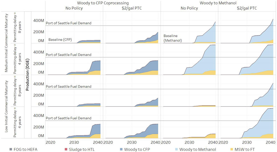
Figure 6. Biofuel production for different pathways, from 2020 to 2040, given differing assumptions on permitting delays, policy, and initial commercial maturity. Reference line shows projected 2040 demand of 307 million DGE at the Port of Seattle.

4 Conclusion

The RBEM analysis presented herein shows the potential for significant fuel demand fulfillment at the Port of Seattle using the biomass-based feedstocks and processing pathways analyzed—but only when feedstock is available and policy incentives are in place to promote the production of marine biofuels. In RBEM, Pathways 1, 2, and 4a are considered feedstock-constrained at a policy level of $2/gal and Pathway 4b is feedstock constrained at all policy levels. This is generally consistent with the FTOT analyses presented for Pathways 1 and 2. RBEM shows more of the port fuel demand could be met by biofuels than FTOT, assuming there is no competition for feedstock from other sectors and if policy is available for marine biofuels. This is an expected result because RBEM does not consider the optimal transportation routing of feedstock and finished fuels. RBEM shows the timing of biofuel deployment could be greatly influenced by feedstock competition, policy incentives, and permitting and construction timelines. These factors could also influence the routing and location of optimal feedstock sources in FTOT results.

RBEM does not consider routing and is not an optimization model. Therefore, its results will differ from those of FTOT. Yet geospatial supply chain analysis with FTOT also suggests alternative fuel supply chains in the PNW could supply significant volumes of marine biofuels to the Port of Seattle based on geospatially explicit feedstock availability and transport cost requirements. The potential demand fulfillment in the FTOT analyses is dominated by sewage-sludge-based HTL fuels at a 10% blend level (without upgrading), a blending constraint that is not applied in the RBEM modeling. Wood-residue-based fuels (via CFP or methanolization) could fulfill 7%–14% of demand, MSW 7% of demand, and HEFA 0.9% of demand based on feedstock transport constraints and fuel production techno-economics. The combination of these fuels could fulfill 81.9% of forecasted demand at the Port of Seattle.

This study, to the authors’ knowledge, is a first of its kind evaluation of region-specific supply chains for marine biofuels in the U.S. A prior analysis from the Netherlands, which does not include system dynamics analysis in its methodology concluded similarly for the port of Rotterdam–that the available supply of biomass can meet port fuel demand. However, the regions considered, scale of the analysis and pathways modeled differ significantly from this study.

This analysis shows the importance of considering multiple types of constraints when estimating performance potential for alternative fuels at a given destination. Future work could further investigate demographic and policy factors that may impact facility siting in FTOT and consider blending constraints in RBEM. Additional analyses at other ports and the potential for expanded supply chain geographies could be explored in both tools to add to the larger context in which these regional supply chains will develop.

Data availability statement

The original contributions presented in the study are included in the article/Supplementary Material, further inquiries can be directed to the corresponding author.

Author contributions

SA: Conceptualization, Methodology, Formal Analysis, Writing – original draft. KZ: Conceptualization, Methodology, Formal Analysis, Writing – original draft. KK: Formal Analysis, Writing – original draft. KL: Conceptualization, Methodology, Writing – original draft. EN: Conceptualization, Methodology, Project administration, Writing – original draft. DC: Data curation, Writing – review and editing. SP: Conceptualization, Methodology, Writing – review and editing.

Funding

The author(s) declare that financial support was received for the research and/or publication of this article. This work was authored by the National Renewable Energy Laboratory for the U.S. Department of Energy (DOE) under Contract No. DE-AC36-08GO28308 and by the U.S. Department of Transportation’s Volpe National Transportation Systems Center under an Interagency Agreement with DOE (Contract No. 89243423SEE000152). Funding provided by U.S. Department of Energy Office of Energy Efficiency and Renewable Energy Bioenergy Technologies Office. The views expressed in the article do not necessarily represent the views of the DOE or the U.S. Government. The U.S. Government retains and the publisher, by accepting the article for publication, acknowledges that the U.S. Government retains a nonexclusive, paid-up, irrevocable, worldwide license to publish or reproduce the published form of this work, or allow others to do so, for U.S. Government purposes.

Acknowledgments

We would like to thank Michael Shell and Joshua Messner of the U.S. Department of Energy (DOE) Bioenergy Technologies Office for their support of this work in addition to Danny Inman, Dan Bilello and Emily Horvath (NREL) and Gregg Fleming, Daniel Flynn, and Erika Sudderth (Volpe) for reviewing versions of this paper. We would also like to offer our gratitude to Kristin Brandt (Washington State University) and Anelia Milbrandt (NREL) for providing feedstock data and Eric Tan, Nick Carlson, and Mike Talmadge (NREL) for providing techno-economic information.

Conflict of interest

The authors declare that the research was conducted in the absence of any commercial or financial relationships that could be construed as a potential conflict of interest.

Generative AI statement

The author(s) declare that no Generative AI was used in the creation of this manuscript.

Publisher’s note

All claims expressed in this article are solely those of the authors and do not necessarily represent those of their affiliated organizations, or those of the publisher, the editors and the reviewers. Any product that may be evaluated in this article, or claim that may be made by its manufacturer, is not guaranteed or endorsed by the publisher.

Supplementary material

The Supplementary Material for this article can be found online at: https://www.frontiersin.org/articles/10.3389/fenrg.2025.1550093/full#supplementary-material

References

CMA, C. G. M. (2022b). CMA CGM and Electrolux make significant move toward sustainable shipping. [WWW Document]. Available online at: https://www.cma-cgm.com/news/4078/cma-cgm-and-electrolux-make-significant-move-toward-sustainable-shipping (Accessed May 21, 24).

Google Scholar

CMA CGM (2022a). CMA CGM launches global biofuel bunkering trial in Singapore. [WWW Document]. Available online at: https://www.cma-cgm.com/news/4082/cma-cgm-launches-global-biofuel-bunkering-trial-in-singapore (Accessed October 4, 23).

Google Scholar

European Commission (2023). Commission welcomes IMO climate ambition [WWW Document]. Maritime transport emissions: Commission welcomes new IMO climate ambition for 2030, 2040 and 2050 and calls to set transition in motion. Available online at: https://ec.europa.eu/commission/presscorner/detail/en/ip_23_3745 (Accessed April 3, 24).

Google Scholar

ExxonMobil (2022). ExxonMobil completes two commercial bio-based marine fuel deliveries. The Maritime Executive.

Google Scholar

ExxonMobil (2024). High science on the high seas. [WWW Document]. High Science on the High Seas. Available online at: https://corporate.exxonmobil.com/What-we-do/Transforming-transportation/lower-emission-fuels/shipping#Workingtoloweremissions (Accessed May 21, 24).

Google Scholar

Gartland, N., and Pruyn, J. (2022). Marine biofuels costs and emissions study for the European supply chain till 2030. Front. Energy Res. 10. doi:10.3389/fenrg.2022.894555

CrossRef Full Text | Google Scholar

Hsieh, C.-W. C., and Felby, C. (2017). Biofuels for the marine shipping sector. IEA Bioenergy.

Google Scholar

IMO Marine Environment Protection Committee (2023). Annex 15, resolution MEPC.377(80), 2023 IMO strategy on reduction of GHG emissions from SHIPS. International Maritime Organization.

Google Scholar

Inman, D., Peterson, S., and Newes, E. (2023). Overview of the regional bio-economy model (RBEM) (No. TP-6A20-85090). Golden, CO: National Renewable Energy Laboratory.

Google Scholar

IRENA (2021). A pathway to decarbonise the shipping sector by 2050. isee systems, 2023. Stella Professional [WWW Document]. Products. Available online at: https://www.iseesystems.com/store/products/stella-professional.aspx (Accessed February 6, 23).

Google Scholar

Kesieme, U., Pazouki, K., Murphy, A., and Chrysanthou, A. (2019). Biofuel as an alternative shipping fuel: technological, environmental and economic assessment. Sustain. Energy Fuels 3, 899–909. doi:10.1039/C8SE00466H

CrossRef Full Text | Google Scholar

Milbrandt, A., and Badgett, A. (2024). Chapter 3: waste resources and byproducts In 2023 Billion-Ton Report. Editor M. H. Langholtz Oak Ridge, TN: Oak Ridge National Laboratory. doi:10.23720/BT2023/2316168

CrossRef Full Text | Google Scholar

Mohd Noor, C. W., Noor, M. M., and Mamat, R. (2018). Biodiesel as alternative fuel for marine diesel engine applications: a review. Renew. Sustain. Energy Rev. 94, 127–142. doi:10.1016/j.rser.2018.05.031

CrossRef Full Text | Google Scholar

Ovcina Mandra, J. (2024). Clarksons: 45% of ships ordered in 2023 embrace alternative fuels, with LNG still in the lead. [WWW Document]. Offshore Energy. Available online at: https://www.offshore-energy.biz/clarksons-45-of-ships-ordered-in-2023-embrace-alternative-fuels-with-lng-still-in-the-lead/(Accessed March 21, 24).

Google Scholar

Saul, J., and Abnett, K. (2021). EU proposes adding shipping to its carbon trading market. [WWW Document]. Reuters. Available online at: https://www.reuters.com/business/sustainable-business/eu-proposes-adding-shipping-its-carbon-trading-market-2021-07-14/(Accessed October 4, 23).

Google Scholar

Simonsen, T. I., Weiss, N. D., van Dyk, S., van Thuijl, E., and Thomsen, S. T. (2021). Progress towards biofuels for marine shipping: status and identification of barriers for utilization of advanced biofuels in the marine sector. IEA Bioenergy.

Google Scholar

Snowden-Swan, L. J., Zhu, Y., Bearden, M. D., Seiple, T. E., Jones, S. B., Schmidt, A. J., et al. (2017). Conceptual biorefinery design and research targeted for 2022: hydrothermal liquefacation processing of wet waste to fuels (No. PNNL--27186, 1415710). doi:10.2172/1415710

CrossRef Full Text | Google Scholar

State of Washington (2021). Vessel to vessel oil transfer.

Google Scholar

Sterman, J., Morrison, J., and Repenning, N. (2003). System dynamics for business policy. [WWW Document]. Sloan School of Management|MIT OpenCourseWare. Available online at: https://dspace.mit.edu/bitstream/handle/1721.1/91162/15-874-fall-2003/contents/index.htm (Accessed October 28, 16).

Google Scholar

Tan, E. C. D., Harris, K., Tifft, S., Steward, Da., and Kinchin, C. (2021a). Adoption of biofuels for the marine shipping industry: a long-term price and scalability assessment (No. NREL/TP-5100-78237). Golden, CO: National Renewable Energy Laboratory.

Google Scholar

Tan, E. C. D., Hawkins, T. R., Lee, U., Tao, L., Meyer, P. A., Wang, M., et al. (2021b). Biofuel options for marine applications: technoeconomic and life-cycle analyses. Environ. Sci. Technol. 55, 7561–7570. doi:10.1021/acs.est.0c06141

PubMed Abstract | CrossRef Full Text | Google Scholar

Tan, E. C. D., and Kaul, B. C. (2023). Bio-intermediates and bio-residuals as marine fuels (Washington D.C.: Advanced Bioeconomy Leadership Conference).

Google Scholar

UNCTAD (2022). Review of Maritime Transport 2022: Navigating stormy waters. United Nations. (Geneva: Elsevier), Available online at: https://unctad.org/system/files/official-document/rmt2022_en.pdf

Google Scholar

Volpe National Transportation Systems Center (2024). Freight and fuel transportation optimization tool (FTOT) Cambridge, MA.

Google Scholar