Application of quasi-oppositional driving training-based optimization for a feasible optimal power flow solution of renewable power systems with a unified power flow controller

The current study’s objective is to reveal the best possible solution for an optimal power flow (OPF) problem. The driving training-based optimization (DTBO) technique has been applied in this work to achieve the goal where quasi-oppositional based learning (QOBL) has been integrated with DTBO and referred to as quasi-oppositional driving training-based optimization (QODTBO). The experiments have been carried out on IEEE 57 & 118 bus systems. Four different test scenarios have been considered here. The first one is the traditional IEEE 57 bus network; the IEEE 57 bus with renewable energy sources (RESs) (i.e., solar and wind units) is chosen in the second one, and the third one considers the IEEE 57 bus with RESs and unified power flow controller (UPFC) and finally the IEEE 118 bus network with RESs and UPFC. In each test scenario, there are four objective functions, among which one is single objective and three of them are multi-objective. Obtaining minimum total cost comes under the single-objective function. Simultaneous reduction in the overall cost and emission, concurrent reduction in overall cost and voltage deviation (VD), and simultaneous reduction in overall cost and voltage stability index come under multi-objective cases. The acquired test outcomes by QODTBO have been contrasted with the outcomes found by the use of DTBO, backtracking search optimization algorithm (BSA), and sine cosine algorithm (SCA). The effect of inherent uncertainties within RESs is gauged in the current study by the choice of appropriate probability density functions (PDF). Based on the experimental outcomes using different optimization techniques over thirty trials, a statistical report has been prepared that ascertains that QODTBO is the most robust optimization scheme among the optimization tools taken into consideration in this study. To represent the statistical analysis, pictorially box plots and error-bar plots are provided. One-way analysis of variance (ANOVA) tests have also been conducted on test outcomes to enhance the degree of reliability of the inferences made based on statistical results. From this work, it is also explored that integrating RESs and UPFC with the traditional IEEE-57 bus system can improve the overall execution of the test system. If the performances of the conventional system, RES-based system, and RES- and UPFC-based system are observed, it can be noticed that for cost reduction, the RES-based system gives a better result by 1.364790635% and the RES- and UPFC-based system gives a better result by 2.175247484% better result as compared to the conventional system.

1 Introduction

Mitigating the issue of the optimal power flow (OPF) (Burchett et al., 1984) has become an indispensable challenge in the current energy system scenario for the sake of satisfactory electric power production, operation, monitoring and control. OPF is an inherent non-linear problem. The objective of the OPF is to obtain an optimal solution for the design variables of the grid or network that minimizes the objective function under several operating constraints. Design variables include the active power of the generator, generator voltage, and transformer tap settings of the transformer. The capacity of the generators, the equations of power flow, the thermal limit of the lines, the limits of the bus voltage, etc. belong to system constraints. Objective functions may belong to single- or multi-objective categories (Roy and Mandal, 2012). In the single-objective category, there is only one objective to be fulfilled, while in the multi-objective category, simultaneously more than one objective has to be met. These goals can include minimizing the fuel costs of power generation, reducing power plant emissions, reducing power losses, and improving voltage stability (Roy et al., 2012). It is very evident that conventional energy resources stocks are decreasing over time. In addition to that, conventional energy sources, such as fossil fuels, have an adverse effect on the atmosphere. These lead to an increase in the usage of RESs (Riaz et al., 2021). Whenever RESs are introduced with conventional sources, the uncertainties present within RESs become a matter of important concern. To maintain several attributes of power quality, flexible AC transmission system (FACTs) tools have been increasingly used in recent times. Incorporating RES and FACTs devices with the existing network increases the overall complexity of the power network.

1.1 Literature review

Several schemes and techniques have been developed for solving OPF issues during the last couple of years. These approaches can be categorized into classical means, evolutionary-based approaches, and methods based on metaheuristic algorithms (Riaz et al., 2021).Numerical approaches like the interior point algorithm (Yan and Quintana, 1999), Newton–Raphson algorithm (Zhang and Irving, 1994; Sun et al., 1984), linear programming (Olofsson et al., 1995), and quadratic programming (Burchett et al., 1984), referred as classical approaches, were being used for resolving OPF problems. But these conventional methods have some severe demerits such as prolonged computational periods and sticking into local optimums instead of global optimums (Mohamed et al., 2021). Existing non-linearities within the OPF problem also reduce the effectiveness of these methods. In the evolutionary algorithm, the best possible solutions are computed by the concept of evolution where the next generation is produced by the process of matting from parentages. To find OPF solutions, two widespread evolutionary algorithms genetic algorithm (Devaraj and Yegnanarayana, 2005), (Moeini-Aghtaie et al., 2014), (Bakirtzis et al., 2002), and differential evolution (Biswas et al., 2018a) are employed. Optimization algorithms that are developed from the social activities of living species or the physical rules of nature are metaheuristic algorithms, for example, particle swarm optimization (PSO) (Ben Attous and Labbi, 2009), whale optimization algorithm (WOA) (Papi Naidu et al., 2021), the moth-swarm algorithm (MSA) (Ali Mohamed et al., 2017), elephant herding optimization (EHO) (Bentouati et al., 2017), gray wolf optimization (GWO) (Siavash et al., 2017a), and gravitational search algorithm (GSA) (Roy et al., 2012).

Various optimization techniques found in literature which were used to resolve OPF problems are presented below. The effectiveness of the modified sine–cosine algorithm on different types of IEEE bus systems to improve economic and operational aspects has been inspected by Attia et al. (2018). To find the solution to OPF issues, the PSO-based fuzzy satisfaction maximization technique is adopted in Surender Reddy (2017). In Bouchekara et al. (2016), improved colliding bodies optimization was presented. Siavash et al. (2017b) demonstrated that the application of GWO to resolve the OPF issue considering the wind unit gave superior results than the use of the genetic algorithm. Ullah Khan et al. (2020) had also utilized GWO to solve OPF issues for different bus systems. To minimize power loss in transmission lines, minimize the operating cost, and improving voltage stability, the teaching learning-based optimization algorithm has been implemented by Maheshwari et al. (2022) on the modified IEEE 30-bus test system including RESs (solar, wind and tidal energy systems). For RESs on the IEEE 30-bus, by using jellyfish search (JS) optimizer, Farhat et al. (2021) have minimized the total generation cost. Guvenc et al. (2021) had tested the distance balance-based adaptive guided differential evolution (AGDE) algorithm on the IEEE 30 node test system including RESs. To solve the OPF problem (for minimizing emission, the fuel cost, voltage deviation, and real power loss), the utility of the equilibrium optimizer technique (EO) was examined by Nusair and Alhmoud (2020), where solar photovoltaic (PV) and wind are integrated. Over different bus systems, Shaheen et al. (2021) had applied the Chaotic hunger games search (CHGS) optimization algorithm for minimizing fuel cost and appropriate positioning of RESs. In Alasali et al. (2021), manta ray foraging optimization (MRFO) had been utilized to obtain feasible OPF with RESs included. The flower pollination algorithm was tested by Abdullah et al. (2020). Over several IEEE bus systems, the performance of the modified JAYA algorithm has been inspected by Elattar and ElSayed (2019) to extract the best possible solution. To find optimal results on different bus test systems, Shaheen $etal$ have used the heap optimization algorithm in (Mohamed et al., 2021) and considered RESs. Biogeography-based optimization was tested by Mosbah et al. (2018) to curtail power losses and to achieve the optimal size and location of photovoltaic-based DG. In Shilaja (2021), cost- and time-effective solutions have been shown for IEEE buses of 30 & 57 using chaotic PSO and GSA. The use of levy coyote optimization to satisfy multiple objectives in the OPF (having RESs on the IEEE 30/57/118 bus system) is shown by Kaymaz et al. (2021). Duman et al. (2021) have tested the symbiotic organisms search algorithm on numerous IEEE bus systems where RESs (solar, wind, and tidal) had been taken into account. Hoang Bao Huy et al. (2022) suggested the multi-objective group search algorithm (MOSGA) to solve the OPF issue on IEEE 30-bus and 57-bus systems with solar and wind energy aiming to reduce emissions, real power loss, and total cost. Pandya and Jariwala (2020) suggested use of non-dominated sort multi-objective GWO for solving the OPF problem with RESs (wind and solar) on the IEEE-30 bus system. To minimize generation cost, power loss, and simultaneously cost and emission, barnacles mating optimizer has been tried on modified IEEE 30 & 57-bus systems by Herwan Sulaiman and Mustaffa (2021). To solve the OPF problem, the competence and firmness of the circle search algorithm have been verified by Shaheen et al. (2022) on the IEEE 57 & 118-bus test network allied with RESs (wind and solar). Targeting to reduce total fuel cost, total emission, voltage magnitude deviation, and active power loss, Kumar Avvari and Vinod Kumar (2022) have offered a new multi-objective evolutionary algorithm which is established on hybrid decomposition, for IEEE 30, 57 & 118 bus systems associated with RESs (solar and wind) and its needful PDFs to handling its uncertainties. The mayfly algorithm has been employed to reduce power loss, fuel cost, emissions, and keep voltage security index (VSI) on the 30 bus with RESs (solar and wind) in order to solve the OPF problem by Khamees et al. (2023). In most of the systems where RESs are included, appropriate PDFs like lognormal, Weibull, and Gumbel were considered to overcome the volatility within RESs (Maheshwari et al., 2022), (Nusair and Alhmoud, 2020), (Duman et al., 2021), (Kumar Avvari and Vinod Kumar, 2022), (Khamees et al., 2023). Hybridization of more than one optimization technique is done often to enhance the searching ability globally. The heftiness and performance of the joined PSO-GWO algorithm on the modified IEEE 30-bus containing RESs (solar and wind) have been verified by Riaz et al. (2021). Alghamdi $etal$ had carried out combined firefly and JAYA algorithms (Ali, 2022) to solve the OPF problem for a 30-bus IEEE network. Ullah et al. (2019) have attained the OPF results via mutual phasor PSO and glowworm swarm optimization (GSO) on the IEEE 30-bus test system with RESs (solar and wind). Annapandi et al. (2021) have described the OPF problem using combined spotted hyena optimization and EHO including RESs (wind and solar), battery, and fuel cell. Hassan et al. (2024) applied a hybrid approach for solving the OPF problem with the consideration of RESs like wind, solar, and electric vehicle (EV) for optimal solutions. The enhanced wombat optimization algorithm has been used by Nagarajan et al. (2025) to find OPF solutions under RESs and EV-based power network. Hassan et al. (2023) used the hybrid AEO-CGO algorithm Hassan $etal$ to resolve RESs including the OPF issue. Optimization of proton exchange membrane fuel Cell (PEMFC) models through the depth information-based differential evolution (Di-DE) algorithm was performed by Jangir et al. (2024a). Mutational Northern goshawk and Elite opposition learning-based artificial rabbits optimizer (MNEARO) was used by Jangir et al. (2024b) in their recent endeavor employing enhanced versions of the artificial hummingbird algorithm, as shown in Jangir et al. (2024c). In Jangir et al. (2025), a cooperative strategy-based differential evolution algorithm is utilized. In order to solve the stochastic OPF problem with optimal integration of RESs and a thyristor controlled series compensator (TCSC), Mohamed et al. (2023) suggests a modified version of the Runge Kutta optimizer (MRUN). Adaptive Lightning Attachment Procedure Optimizer (ALAPO) with RES integration was used by Adhikari et al. (2023) study to solve the stochastic OPF problem. Ebeed et al. (2018) performed a thorough analysis of contemporary optimization methods for resolving optimal power flow issues Ebeed $etal$. In order to solve the issues of the normal Gorilla Troops Optimizer being susceptible to local optima and the potential for stagnation, Jamal et al. (2024) using suggests an effective modified Gorilla Troops Optimizer. Zhang et al. (2024) suggests an approach for calculating OPF that takes demand-side responsiveness and RES uncertainty into account. An enhanced chaotic flower pollination algorithm was presented by Daqaq et al. (2022) in order to address the OPF problem by incorporating RESs and producing the best control variable settings. An optimal power flow model that accounts for the uncertainty in the probability distribution of wind power was proposed by Dai et al. (2024).

Contemporary researchers are engaged in solving OPF problems considering FACTs tools within the system, which improves the power quality attributes. In the following part, few such studies are presented. In the OPF problem, optimal positioning and sizing of certain FACTS devices were accomplished by Amal et al. (2022) using a hybrid gradient-based optimizer with moth–flame optimization algorithm. Fruitful placement and sizing of the FACTS devices in the IEEE 30-bus system (including wind farms) for lessening transmission costs, generation costs, and power losses and concurrently protecting voltage profile were analyzed by Aghaebrahimi et al. (2016) using honey-bees mating optimization. To resolve difficult nonlinear OPF problems for the IEEE 30-bus test system integrating RES and FACTs devices, Nusair et al. (2021) tested four biology and nature-inspired optimization algorithms, namely, artificial ecosystem-based optimization (AEO), slime mold algorithm (SMA), JS, and marine predators algorithm (MPA). GWO-based optimal tuning has been implemented by Rambabu et al. (2019) to find the optimal power flow solution considering FACTs devices and RESs on the IEEE 57-bus system. Panda et al. (2017) had revealed the advantage of using the modified bacteria foraging algorithm to solve the OPF problem (combined hydro-thermal-wind (HTW) system with shunt fact devices). Duman et al. (2020) resolved the OPF problem with use of FACTS devices and that of uncertain wind energy unit had resolved using hybrid PSO and GSA (PSOGSA) with chaotic maps Duman $etal$. Biswas et al. (2021) employed the history-based adaptive differential evolution algorithm to achieve the best OPF solution where the IEEE 30 bus system was considered with RES and FACTs tools.

1.2 Research gaps

1. Local optimum problems plague the majority of current optimization approaches.

2. The majority of optimization strategies currently in use suffer from computational complexity.

3. The majority of current optimization algorithms have not yet been implemented on large-scale grids connecting FACTs and renewable energy-based network.

4. For scheduling a greater number of renewable energy sources with more nonlinearity, the majority of current optimization algorithms have not been validated on complicated systems.

5. Analysis of variance (ANOVA), box plot, and error bar were not used in the majority of optimizations to determine the means of the data that were produced.

6. Statistical analysis is not used to discuss the robustness of the majority of current algorithms.

7. Instead of applying applied to multi-objective functions, the majority of optimization techniques were focused on single-objective functions.

8. Most of the existing systems do not test error bar analysis, which aids in calculating the standard deviation and standard errors to validate the value of the maximum and minimum ranges.

1.3 Motivation and incitement

According to the literature review, the existing optimization strategies have the following features:

1. Effective solutions to many non-linear-based problems.

2. There are no derivatives associated in the population-based optimization methods mentioned above.

3. Robustness can be demonstrated for most of the current approaches.

In this presentation, authors were motivated to employ a new optimization method to overcome the previously described drawbacks.

1.4 Contribution

The following are the primary contributions of this research work:

• The proposed study adopts a new approach for solving the OPF-based combined heat and power economic dispatch (CHPED) problem of IEEE 57 and IEEE 118 bus systems.

•Suggested study integrates wind–solar units with two OPF-/CHPED-based systems, namely, IEEE 57 and IEEE 118 buses, considering the significance of the fossil fuel source’s constant evolution.

•Moreover, the FACTS device UPFC has been integrated with the wind–solar-based OPF system on IEEE 57 and IEEE 118 bus systems.

•To cope up with these non-linearities, a new approach QODTBO is implemented on the proposed work that provides optimal solutions over cost and emission with a fast convergence rate.

•The suggested optimization technique’s robustness has been assessed using statistical analysis.

•An analysis of variance (ANOVA) test, box plot, and error bar plots are used for scrutiny in a rigorous manner so that the robustness of QODTBO may be assessed more accurately.

•An analysis has been conducted by comparing the proposed QODTBO algorithm with efficient optimization methods in order to address its superiority.

The suitability of any optimization algorithm is dependent on the nature of the optimization problem. So the upgradation of algorithms or development of new algorithms is always an ongoing process so as to increase the effectiveness of the optimization technique to reach numerous objectives of the OPF problem. In the current study, there are three types of test systems. In the first type, a simple IEEE 57 bus system has been chosen, the IEEE 57 bus integrated with RESs (Wind–PV unit) is adopted as the second type test system, and in the third type of test system, the IEEE 57 bus is studied with RESs and UPFC. Single- and multi-task objectives are addressed here. The briefs of the test systems and the set objectives are provided in Table 1. The objectives of the present study are minimization of the generation cost, simultaneous minimization of total cost and emission, concurrent reduction of generation cost and improvement in the voltage profile, and simultaneous minimization of the generation cost and the voltage stability index. In the present study, a newly developed optimization technique DTBO (Dehghani et al., 2022) is employed. The method has been established recently based on driving training courses for human beings. DTBO maintains a decent balance between exploitation and exploration. Dehghani et al. (2022) have revealed that DTBO offers enhanced performances in optimization applications than 11 other contestant algorithms. To make the response faster and obtain a superior optimal solution based on quasi-oppositional learning (QOBL), Warid et al. (2018) integrated it with the original DTBO, which is referred to as quasi-oppositional DTBO (QODTBO). It will explore the search region more proficiently and avoid getting stuck in a native solution. The test results obtained have been compared with the results obtained by Chaib et al. (2016).

Table 1

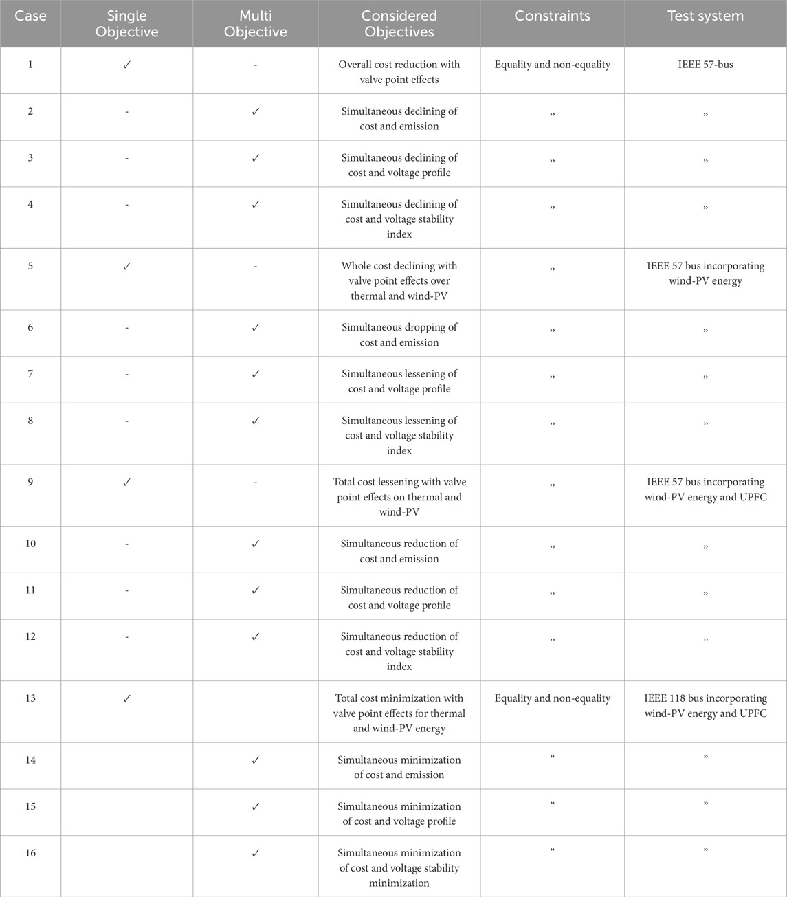
Table 1. Summaries of different case studies under consideration.

1.5 Limitation of the QODTBO approach

The following are the limitations of the QODTBO approach.

1. Though the suggested approach has the potential to refine near-optimal solutions globally, it may be hybridized with other counterparts to further accelerate its searching capability.

2. The performance of the algorithm is crucially dependent on the choice of input control parameters.

3. There is a scope of population diversification

4. Challenges may arise when a very high-dimensional optimization problem is to be resolved.

1.6 Organization of the paper

The remaining sections of this paper are organized as follows: Section 2 includes a model of the FACTs devices, wind power, and solar power generation. In Section 3, formulation of the problem of the proposed system is demonstrated. Section 4 includes a flowchart and a discussion of the various steps of the suggested optimization approach. The benchmark functions and simulation results are covered in Section 5, along with a comparison of multiple examples using statistical analysis. Section 6 of the proposed system reports the conclusion. The design frame of the proposed research work is illustrated in Figure 1.

Figure 1

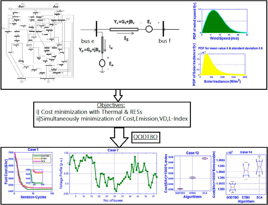
Figure 1. Design framework of the proposed research work.

2 Model: FACTs devices and RESs

2.1 Modeling of UPFC

To control power transmission networks, UPFC (Dutta et al., 2015) is considered the best FACTs tool. It is adaptive in nature. It can regulate both active and reactive power flows within the terminals. It also compensates for reactive power at the linked node (Gyugyi, 1992), (Abdollahi et al., 2020). In this device, there are series and shunt-connected voltage source converters that have a common direct current (DC) link. The series part of the device is similar to the static synchronous series compensator (SSSC), while the shunt part resembles that of the static compensator (STATCOM). Figure 2 depicts the UPFC tool, which is placed between the $e^{th}$ & $f^{th}$ buses.

Figure 2

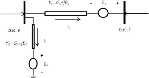
Figure 2. Circuit model for the UPFC.

The injected active and reactive power of the $e^{th}$ & $f^{th}$ buses are given by (Dutta et al., 2015); (Radman and Raje, 2007) Equations 1–4:

$\left\{\begin{array}{c}{P}_e=\left(G_P+G_S\right){\left|V_e\right|}^2-\left|V_e\right|\left|E_p\right|\left|Y_p\right|\cos \left({\theta }_p-{\delta }_e+{\delta }_p\right)\hfill \\ +\left|V_e\right|\left|E_s\right|\left|Y_s\right|\cos \left({\theta }_s+{\delta }_s-{\delta }_e\right)\hfill \\ -\left|V_f\right|\left|V_f\right|\left|Y_s\right|\cos \left({\theta }_s-{\delta }_e+{\delta }_f\right)\hfill \\ +{\displaystyle \sum _{k=1}^{NB}}\left|V_e\right|\left|V_f\right|\left|Y_{ef}\right|\cos \left({\theta }_{ef}-{\delta }_e+{\delta }_f\right)\hfill \end{array}\right..(1)$

$\left\{\begin{array}{c}{Q}_e=-\left(B_P+B_S\right){\left|V_e\right|}^2+\left|V_e\right|\left|E_p\right|\left|Y_p\right|\sin \left({\theta }_p-{\delta }_e+{\delta }_p\right)\hfill \\ -\left|V_e\right|\left|E_s\right|\left|Y_s\right|\sin \left({\theta }_s+{\delta }_s-{\delta }_e\right)\hfill \\ +\left|V_e\right|\left|V_f\right|\left|Y_s\right|\sin \left({\theta }_s-{\delta }_e+{\delta }_f\right)\hfill \\ +{\displaystyle \sum _{k=1}^{NB}}\left|V_e\right|\left|V_k\right|\left|Y_{fk}\right|\sin \left({\theta }_{ek}-{\delta }_f+{\delta }_k\right)\hfill \end{array}\right..(2)$

$\left\{\begin{array}{c}{P}_f=G_S{\left|V_f\right|}^2-\left|V_f\right|\left|V_e\right|\left|Y_s\right|\cos \left({\theta }_s-{\delta }_f+{\delta }_e\right)\hfill \\ -\left|V_f\right|\left|E_s\right|\left|Y_s\right|\cos \left({\theta }_s+{\delta }_s-{\delta }_e\right)\hfill \\ +{\displaystyle \sum _{k=1}^{NB}}\left|V_f\right|\left|V_k\right|\left|Y_{fk}\right|\cos \left({\theta }_{fk}-{\delta }_f+{\delta }_k\right)\hfill \end{array}\right..(3)$

$\left\{\begin{array}{c}{Q}_f=-B_S{\left|V_f\right|}^2+\left|V_f\right|\left|V_e\right|\left|Y_s\right|\sin \left({\theta }_s-{\delta }_f+{\delta }_p\right)\hfill \\ -\left|V_f\right|\left|E_s\right|\left|Y_s\right|\sin \left({\theta }_s+{\delta }_s-{\delta }_f\right)\hfill \\ +{\displaystyle \sum _{k=1}^{NB}}\left|V_f\right|\left|V_k\right|\left|Y_{fk}\right|\sin \left({\theta }_{ek}-{\delta }_f+{\delta }_k\right)\hfill \end{array}\right..(4)$

Due to presence of the UPFC, the flow of active and reactive power (Radman and Raje, 2007) through the transmission line placed within $e^{th}$ & $f^{th}$ buses is expressed as follows Equations 5–8:

$\left\{\begin{array}{c}{P}_{ef}=\left(G_P+G_S\right){\left|V_e\right|}^2-\left|V_e\right|\left|E_p\right|\left|Y_p\right|\cos \left({\theta }_p-{\delta }_e+{\delta }_p\right)\hfill \\ +\left|V_e\right|\left|E_s\right|\left|Y_s\right|\cos \left({\theta }_s+{\delta }_s-{\delta }_e\right)\hfill \\ -\left|V_e\right|\left|V_f\right|\left|Y_s\right|\cos \left({\theta }_s-{\delta }_e+{\delta }_f\right)\hfill \end{array}\right..(5)$

$\left\{\begin{array}{c}{Q}_{ef}=-\left(B_P+B_S\right){\left|V_e\right|}^2+\left|V_e\right|\left|E_p\right|\left|Y_p\right|\sin \left({\theta }_p-{\delta }_e+{\delta }_p\right)\hfill \\ -\left|V_e\right|\left|E_s\right|\left|Y_s\right|\sin \left({\theta }_s+{\delta }_s-{\delta }_e\right)\hfill \\ +\left|V_e\right|\left|V_f\right|\left|Y_s\right|\sin \left({\theta }_s-{\delta }_e+{\delta }_f\right)\hfill \end{array}\right..(6)$

$\left\{\begin{array}{c}{P}_{fe}=G_S{\left|V_f\right|}^2-\left|V_f\right|\left|V_e\right|\left|Y_s\right|\cos \left({\theta }_s-{\delta }_f+{\delta }_e\right)\hfill \\ -\left|V_f\right|\left|E_s\right|\left|Y_s\right|\cos \left({\theta }_s+{\delta }_s-{\delta }_e\right)\hfill \end{array}\right..(7)$

$\left\{\begin{array}{c}{Q}_{fe}=-B_S{\left|V_f\right|}^2+\left|V_f\right|\left|V_e\right|\left|Y_s\right|\sin \left({\theta }_s-{\delta }_f+{\delta }_p\right)\hfill \\ -\left|V_f\right|\left|E_s\right|\left|Y_s\right|\sin \left({\theta }_s+{\delta }_s-{\delta }_f\right)\hfill \end{array}\right..(8)$

There is no net power loss in the UPFC, which can be represented as Equation 9,

$\left\{\begin{array}{c}{G}_p{\left|E_p\right|}^2+G_s{\left|E_s\right|}^2-\left|E_p\right|\left|V_e\right|\left|Y_p\right|\times \cos \left({\delta }_p-{\delta }_e-{\theta }_p\right)\hfill \\ +\left|E_s\right|\left|V_e\right|\left|Y_s\right|\times \cos \left({\delta }_s-{\delta }_e-{\theta }_s\right)\hfill \\ -\left|E_s\right|\left|V_f\right|\left|Y_s\right|\times \cos \left({\delta }_s-{\delta }_f-{\theta }_s\right)=0\hfill \end{array}\right.,(9)$

where $V_e,V_f$, respectively, indicate the magnitude of voltages at the $e^{th}$ & $f^{th}$ buses; $G_p$, $B_p$ and $Y_p$ are the parallel component conductance, susceptance, and admittance, respectively. The overall admittance of the transmission line present between the e–f bus and the series component of the UPFC is $Y_s$, the UPFC series component’s conductance and susceptance are respectively; the admittance angle of the transmission line positioned between Gs, BS $e^{th}$ and $f^{th}$ bus is ${\theta }_{ef}$; the admittance angle between the admittance of the UPFC series component and the admittance that contains the admittance of the line e–f is ${\theta }_s$; the phase angles of the UPFC’s parallel and series component voltage source are the ${\delta }_p$ and ${\delta }_s$, respectively; the voltages of the parallel and series converter’s voltage sources of the UPFC device are $E_p,E_s$, respectively.

2.2 Wind power model

Wind speed $(vm/s)$ (Paul et al., 2024a) fluctuation is well characterized (Rambabu et al., 2019; Duman et al., 2020) by two-parameter (scale factor “$\xi$” and shape factor “$\kappa$”) Weibull PDF as Equation 10,

$f\left(v\right)=\left(\frac{\kappa }{\xi }\right)\times {\left(\frac{v}{\xi }\right)}^{\kappa -1}\times \left({e^{-\left(\frac{v}{\xi }\right)}}^{\kappa }\right)0<v<\infty (10)$

The output power from a wind turbine is given in terms of cut-in speed $v_{in}$, rated speed $v_r$, cut-out speed $v_{\mathit{out}}$, and rated output of the wind turbine $P_{wr}$ as Equation 11,

$P_w\left(v\right)=\left\{\begin{array}{c}0\hfill \\ P_{wr}\left(\frac{v-v_{in}}{v_r-v_{in}}\right)\hfill \\ P_{wr}\hfill \end{array}\begin{array}{c}forv<v_{in}\&v>v_{\mathit{out}}\hfill \\ for{v}_{in}\le v\le v_r\hfill \\ for{v}_r<v\le v_{\mathit{out}}\hfill \end{array}.\right.(11)$

Now, the probabilities of wind power at the distinct wind speed zone can be described by Equations 12–14,

$f{\left(P_w\right)}_{\left|P_w=0\right.}=1-\exp \left[-{\left(\frac{v_{in}}{\xi }\right)}^{\kappa }\right]+\exp \left[-{\left(\frac{v_{\mathit{out}}}{\xi }\right)}^{\kappa }\right].(12)$

$f{\left(P_w\right)}_{\left|P_w=P_{wr}\right.}=\exp \left[-{\left(\frac{v_r}{\xi }\right)}^{\kappa }\right]-\exp \left[-{\left(\frac{v_{\mathit{out}}}{\xi }\right)}^{\kappa }\right].(13)$

$\begin{array}{cc}\hfill & f{\left(P_w\right)}_{\left|0<P_w<P_{wr}\right.}=\left[\frac{\kappa \times \left(v_r-v_{in}\right)}{{\xi }^{\kappa }\times P_{wr}}\right]\times {\left[v_{in}+\left(\frac{P_w}{P_{wr}}\right)\left(v_r-v_{in}\right)\right]}^{\kappa -1}\hfill \\ \hfill & \times \exp \left[-{\left(\frac{v_{in}+\left(\frac{P_w}{P_{wr}}\right)\times \left(v_r-v_{in}\right)}{\xi }\right)}^{\kappa }\right]\hfill \end{array}.(14)$

2.3 Solar power model

In the solar power unit, solar energy (Paul et al., 2024a) is converted to electrical energy. Power output depends on solar irradiance and other climatic conditions. The probability distribution L(I) of solar irradiance (I) is very much close with (Abdullah et al., 2020; Rambabu et al., 2019) lognormal PDF, so it is commonly used to estimate the solar irradiance, and it is represented as Equation 15,

$L\left(I\right)=\frac{1}{I\lambda \sqrt{2\pi }}\exp \left(\frac{-{\left(\ln I-\epsilon \right)}^2}{2{\lambda }^2}\right),I>0(15)$

$\epsilon$: mean of $I$ distribution.

$\lambda$: Standard deviation.

The relation between solar irradiance and the electrical output power from the PV unit is given by Equation 16,

$P\left(I\right)=\left\{\begin{array}{c}{P}_{nm}\frac{I^2}{I_{st}{I}_c},for0<I<I_c\hfill \\ P_{nm}\frac{I}{I_{st}},forI\ge I_c\hfill \end{array}\right.(16)$

$P_{nm}$: nominal output power of the PV unit; $I_{st}$: standard solar irradiance; $I_c$: critical irradiance point.

3 Mathematical problem formulation

3.1 Cost model of thermal power generation

The cost model of fossil fuel-driven thermal units (Biswas et al., 2018b; Rambabu et al., 2019; Pandya and Jariwala, 2020) is usually considered a quadratic function. The generation cost in $/hour unit is given by Equation 17,

$C_{\mathit{T}1\mathit{k}}\left(P_{\mathit{TGk}}\right)=a_k+b_k{P}_{\mathit{TGk}}+c_k{P}_{\mathit{TGk}}^2.(17)$

$a_k$, $b_k$, and $c_k$ are the cost coefficients for $k^{th}$ thermal unit and generated power $P_{T{G}_k}$. While the valve-point loading effect is taken into consideration, generation cost $/h of the $k^{th}$ thermal unit becomes Equation 18,

$\left\{\begin{array}{c}{C}_{\mathit{T}2\mathit{k}}\left(P_{\mathit{TGk}}\right)=\left(a_k+b_k{P}_{\mathit{TGk}}+c_k{P}_{\mathit{TGk}}^2\right)\hfill \\ +\left|d_k\times \sin \left(e_k\times \left(P_{\mathit{TGk}}^{\min }-P_{\mathit{TGk}}\right)\right)\right|\hfill \end{array}\right.(18)$

$d_k$ and $e_k$ are the coefficients related to valve-point loading. $P_{\mathit{TGk}}^{\min }$ is the minimum output power of the $k^{th}$ thermal unit. Table 2 provides the cost coefficients of all thermal units.

Table 2

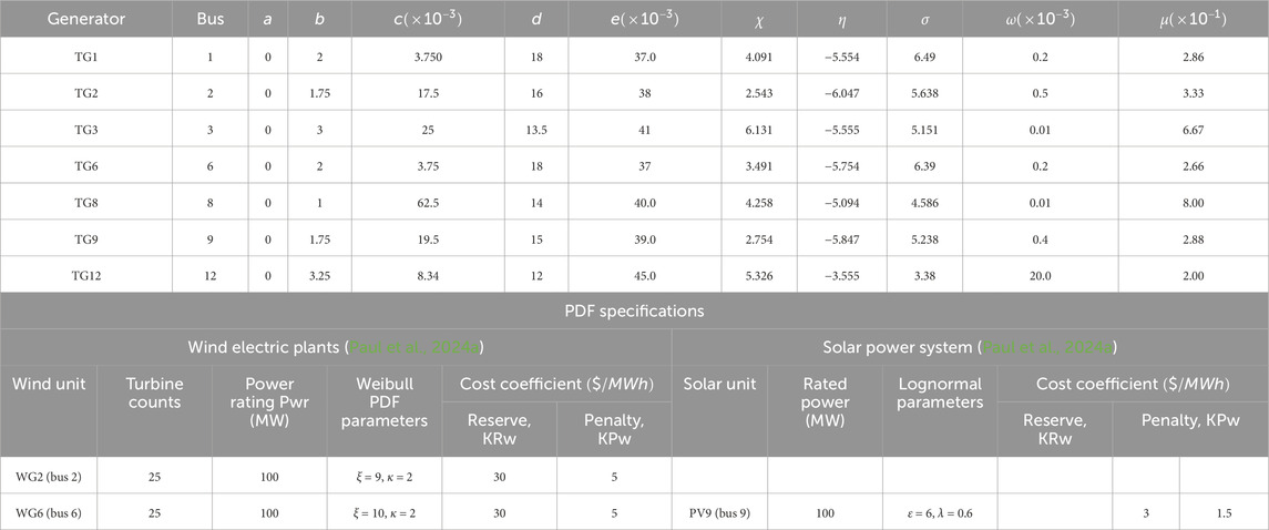
Table 2. Thermal generators’ costs and emission coefficients for the IEEE 57-bus (Paul et al., 2024a) test system and statistical parameters for the distribution of wind velocity and solar irradiance, power rating of wind and PV units, and allied cost coefficients.

3.2 Direct cost of PV and wind power generating unit

In the PV and wind power unit, there is no fuel cost because no fuel is required for the said units. In this kind of power, a direct cost that is proportional to the scheduled power is provided by the grid operators to the owner of PV or wind plants (Kumar Avvari and Vinod Kumar, 2022). In terms of scheduled power $P_{\mathit{ssl}}$, the direct solar power cost for $l^{th}$ PV unit is given by Equation 19,

$C_{sl}\left(P_{\mathit{ssl}}\right)={\gamma }_{sl}{P}_{\mathit{ssl}}(19)$

${\gamma }_{sl}$: coefficient of the direct cost for the $l^{th}$ PV unit.

Similarly, the direct cost for the $k^{th}$ wind power unit is given by Equation 20,

$C_{wk}\left(P_{\mathit{wsk}}\right)={\rho }_{wk}{P}_{\mathit{wsk}}(20)$

${\rho }_{wk}$: coefficient of direct cost for the $k^{th}$ wind power unit.

$P_{\mathit{wsk}}$: scheduled power from the $k^{th}$ wind power unit.

3.3 Cost assessment of wind power uncertainties

Uncertainties are inherent in wind power. While actual produced wind power is less than the scheduled power ($P_{\mathit{wsk}}$) ($i.e$ overestimated wind power), to mitigate the demand, the cost associated with reserve generating units has to be considered, which is called reserve cost (Kumar Avvari and Vinod Kumar, 2022). It can be represented as Equation 21,

$\left\{\begin{array}{c}{C}_{\mathit{Rwk}}\left(P_{ws,k}-P_{\mathit{wavk}}\right)=K_{\mathit{Rwk}}\left(P_{\mathit{wsk}}-P_{\mathit{wavk}}\right)\hfill \\ =K_{\mathit{Rwk}}\underset{0}{\overset{P_{\mathit{wsk}}}{\int }}\left(P_{\mathit{wsk}}-p_{wk}\right)f_w\left(p_{wk}\right)d{p}_{wk}\hfill \end{array}\right..(21)$

$K_{\mathit{Rwk}}$: coefficient of reserve cost for the $k^{th}$ wind power unit; $P_{\mathit{wavk}}$: available power from the $k^{th}$ wind power unit; $f_w\left(p_{wk}\right)$: PDF of the $k^{th}$ wind power plant.

On the other hand, while the actual power from the wind power plant is higher than the scheduled power ($i.e$ underestimation of wind power), there will be a penalty cost to be paid. The penalty cost for the $k^{th}$ wind power unit due to wind power underestimation is represented as Equation 22,

$\left\{\begin{array}{c}{C}_{\mathit{Pwk}}\left(P_{\mathit{wavk}}-P_{\mathit{wsk}}\right)=K_{\mathit{Pwk}}\left(P_{\mathit{wavk}}-P_{\mathit{wsk}}\right)\hfill \\ =K_{\mathit{Pwk}}\underset{P_{\mathit{wsk}}}{\overset{P_{\mathit{wrk}}}{\int }}\left(p_{wk}-P_{\mathit{wsk}}\right)f_w\left(p_{wk}\right)d{p}_{wk}\hfill \end{array}\right..(22)$

$K_{\mathit{Pwk}}$: coefficient of penalty cost for the $k^{th}$ wind power unit. $P_{\mathit{wsk}}$: rated output power from the $k^{th}$ wind power plant.

3.4 Evaluation of cost for solar photovoltaic uncertainties

Similar to the wind power unit, uncertainty is involved with the solar PV unit where both cases of over- and underestimation of solar power may occur. So, in the case of the solar PV unit, reserve and penalty costs have to be considered like wind power units. Solar radiation distribution is close to the lognormal PDF, whereas wind speed matches closely with Weibull PDF. Therefore, reserve and penalty cost functions for the solar PV unit is different from those of the wind power unit.

The reserve cost of the $l^{th}$ solar unit can be shown as Equation 23,

$\left\{\begin{array}{c}{C}_{\mathit{Rsl}}\left(P_{\mathit{ssl}}-P_{\mathit{savl}}\right)=K_{\mathit{Rsl}}\left(P_{\mathit{ssl}}-P_{\mathit{savl}}\right)\hfill \\ =K_{\mathit{Rsl}}\ast f_s\left(P_{\mathit{savl}}<P_{\mathit{ssl}}\right)\ast \left[P_{\mathit{ssl}}-E\left(P_{\mathit{savl}}<P_{\mathit{ssl}}\right)\right]\hfill \end{array}\right.(23)$

$K_{\mathit{Rsl}}$: reserve cost coefficient for the $l^{th}$ PV unit $P_{\mathit{savl}}$: available actual power of the same unit. $P_{\mathit{ssl}}$: power scheduled of that PV unit; $f_s\left(P_{\mathit{savl}}<P_{\mathit{ssl}}\right)$: likelihood of solar power being lower than planned. $E\left(P_{\mathit{savl}}<P_{\mathit{ssl}}\right)$: chances that the PV power is beneath $P_{\mathit{ssl}}$.

The $l^{th}$ PV unit’s penalty cost is shown as Equation 24,

$\left\{\begin{array}{c}{C}_{\mathit{Psl}}\left(P_{\mathit{savl}}-P_{\mathit{ssl}}\right)=K_{\mathit{Psl}}\left(P_{\mathit{savl}}-P_{\mathit{ssl}}\right)\hfill \\ =K_{\mathit{Psl}}\ast f_s\left(P_{\mathit{savl}}>P_{\mathit{ssl}}\right)\ast \left[E\left(P_{\mathit{savl}}>P_{\mathit{ssl}}\right)-P_{\mathit{ssl}}\right]\hfill \end{array}\right.(24)$

$K_{\mathit{Psl}}$: reserve cost coefficient for the $l^{th}$ PV unit; $f_s\left(P_{\mathit{savl}}>P_{\mathit{ssl}}\right)$: probabilities of solar power more than scheduled solar power. $E\left(P_{\mathit{savl}}>P_{\mathit{ssl}}\right)$: expectation that PV power is above $P_{\mathit{ssl}}$.

3.5 Objective function

In the present work, selected objectives (Herwan Sulaiman and Mustaffa, 2021; Biswas et al., 2021; Kumar Avvari and Vinod Kumar, 2022; Chaib et al., 2016) include (a) minimization of total generation cost; (b) upgrading of the voltage profile; (c) improvement in the stability of voltage; (d) reduction of emission. Furthermore, various combinations amid these objective functions are considered too.

3.5.1 Single objective

Total generation cost: (i) when only thermal generators are considered, the total generation cost $(C_{GC})$ is expressed as [using (Equations 18, 25)]

$C_{GC}={\displaystyle \sum _{k=1}^{N_{TG}}}{C}_{\mathit{T}2\mathit{k}}\left(P_{\mathit{TGk}}\right)(25)$

$N_{TG}$ denotes the number of thermal generators. In (Equation 25), the valve-point loading effect is considered.

(ii) The overall generation cost while RESs are taken into account is expressed as [using (Equations 18–24, Equation 26)],

$\left\{\begin{array}{c}{C}_{GC}={\displaystyle \sum _{k=1}^{N_{TG}}}{C}_{\mathit{T}2\mathit{k}}\left(P_{\mathit{TGk}}\right)+{\displaystyle \sum _{k=1}^{N_W}}\left[C_{wk}\left(P_{\mathit{wsk}}\right)\right]\hfill \\ +{\displaystyle \sum _{k=1}^{N_W}}{C}_{\mathit{Rwk}}\left(P_{ws,k}-P_{\mathit{wavk}}\right)+C_{\mathit{Pwk}}\left(P_{\mathit{wavk}}-P_{\mathit{wsk}}\right)\hfill \\ +{\displaystyle \sum _{l=1}^{N_s}}\left[C_{sl}\left(P_{\mathit{ssl}}\right)+C_{\mathit{Rsl}}\left(P_{\mathit{ssl}}-P_{\mathit{savl}}\right)+C_{\mathit{Psl}}\left(P_{\mathit{savl}}-P_{\mathit{ssl}}\right)\right]\hfill \end{array}\right..(26)$

Voltage stability index: In the power system, the extent of voltage stability is a matter of great importance. To gauge it, Kessel and Glavitsch (1986) have introduced the voltage stability index $(L_{\mathit{max}})$, which is given by Equation 27,

$L_{\max }=\max \left(L_k\right)k=\mathrm{1,2},\dots ,N_L,(27)$

where ($L_k$ denotes an local indicator of bus k expressed as Equation 28),

$L_k=\left|1-{\displaystyle \sum _{h=1}^{N_G}}{H}_{L{G}_{kh}}\frac{V_h}{V_k}\right|k=\mathrm{1,2},\dots N_L.(28)$

$N_L$: count of load buses. $N_G$: number of generators.

H: partial inverse matrix of the bus admittance matrix. The magnitude of $L_{\mathit{max}}$ lies between 0 and 1: while it approaches 0, the system stability improves.

Voltage deviation (voltage profile): for load buses to maintain a healthy voltage profile, variations in voltage at load buses have to be minimized, and it is given by Equation 29,

$VD={\displaystyle \sum _{l=1}^{N_L}}\left|V_l-1\right|.(29)$

$N_L$: no of load buses.

Emission: the overall emission of environmental pollutants like carbon dioxide, oxides of sulfur, oxides of nitrogen, etc. triggered by the thermal generators can be represented as Equation 30,

$EC={\displaystyle \sum _{h=1}^{N_{TG}}}{10}^{-2}\left({\chi }_h+{\eta }_h{P}_{\mathit{TGh}}+{\sigma }_h{P}_{\mathit{TGh}}^2\right)+\left({\omega }_h{e}^{\left({\mu }_h{P}_{\mathit{TGh}}\right)}\right).(30)$

Here, ${\chi }_h,{\eta }_h,{\sigma }_h,{\omega }_h\&{\mu }_h$ are emission coefficients of the $h^{th}$ thermal generator. $P_{\mathit{TGh}}$ is the power generated by the $h^{th}$ thermal generator.

3.5.2 Multi-objective

It regularly occurs that the aforementioned objective (minimization) functions are mutually contradicting among themselves. Regularly, in order to get the best possible solution that optimizes those contradictory goals at a time without violating various constraints. These types of optimization issues are referred to as multi-objective optimization problems.

Simultaneously cost and emission minimization: Using (Equations 25, 26, 30) the bi-objective function $(O{F}_{\mathit{comb}1})$ is designed to simultaneously reduce fuel cost and emission. Mathematically, the function can be written as Equation 31,

$O{F}_{\mathit{comb}1}=C_{GC}+{\alpha }_{EC}\left(EC\right).(31)$

${\alpha }_{EC}$ represents the weighting factor corresponding to emission (Chaib et al., 2016).

Combination of generation cost reduction and voltage profile improvement: With the help of (Equations 25, 26, 29), the blended objective function $(O{F}_{\mathit{comb}2})$ to reduce the fuel cost and improve voltage profile can be represented (Chaib et al., 2016) by Equation 32,

$O{F}_{\mathit{comb}2}=C_{GC}+{\alpha }_{vd}\left(VD\right).(32)$

${\alpha }_{vd}$: weighting factor.

${\alpha }_{vd}$ is considered 1000 in this work (Chaib et al., 2016).

Simultaneous minimization of cost and voltage stability index: to achieve an optimum solution such that generation cost and voltage profile index become minimum, we simultaneously combine the objective function $(O{F}_{\mathit{comb}3})$ represented (using (Equations 25–27) as Equation 33,

$O{F}_{\mathit{comb}3}=C_{GC}+{\alpha }_{L_{\mathit{max}}}\left(L_{\mathit{max}}\right).(33)$

${\alpha }_{L_{\mathit{max}}}$ is a weighting coefficient.

3.6 Constraints

While FACTs devices are considered, the OPF constraints (Kumar Avvari and Vinod Kumar, 2022) are provided as follows.

3.7 Equality constraints

Constraint (Equation 34) provides a power flow equation which is shown below Equation 34:

$\left\{\begin{array}{c}{\displaystyle \sum _{c=1}^{N_s}}\left(P_{Gc}-P_{Lc}\right)+{\displaystyle \sum _{c=1}^{N_{\mathit{UPFC}}}}{P}_{cs}={\displaystyle \sum _{c=1}^{N_s}}{\displaystyle \sum _{d=1}^{N_s}}\left|V_c\right|\left|V_d\right|\left|Y_{cd}\right|\cos \left({\phi }_{cd}-{\beta }_{cd}\right)\hfill \\ {\displaystyle \sum _{c=1}^{N_s}}\left(Q_{Gc}-Q_{Lc}\right)+{\displaystyle \sum _{c=1}^{N_{\mathit{UPFC}}}}{Q}_{cs}=-{\displaystyle \sum _{c=1}^{N_s}}{\displaystyle \sum _{d=1}^{N_s}}\left|V_c\right|\left|V_d\right|\left|Y_{cd}\right|\sin \left({\phi }_{cd}-{\beta }_{cd}\right)\hfill \end{array}\right.(34)$

Here $P_{Lc}$ and $Q_{Lc}$ are the active and reactive power demand of the $c^{th}$ bus, respectively; $P_{Gc}$ and $Q_{Gc}$ are the active and reactive power of generation and demand, respectively, of the $c^{th}$ bus; $P_{cs}$ and $Q_{cs}$ are the injected active and reactive power of UPFC, respectively, of the $c^{th}$ bus; $Y_{cd}$ is the admittance of the transmission line connected between the $c^{th}$ and the $d^{th}$ bus; ${\phi }_{cd}$ is the admittance angle of the transmission line connected between the $c^{th}$ and the $d^{th}$ bus; $N_s$ is the number of buses; $N_{\mathit{UPFC}}$ is the number of UPFCs.

3.8 Inequality constraints

All inequality constraints are represented by Equations 35-43,

(i) Generator constraints:

$\left\{\begin{array}{c}\hfill V_{Gb}^{\min }\le V_{Gb}\le V_{Gb}^{\max }\hfill \\ P_{Gb}^{\min }\le P_{Gb}\le P_{Gb}^{\max }b\in N_P\hfill \\ Q_{Gb}^{\min }\le Q_{Gb}\le Q_{Gb}^{\max }\hfill \end{array}\right..(35)$

(ii) Load bus constraints:

$V_{Lb}^{\min }\le V_{Lb}\le V_{Lb}^{\max }\begin{array}{cc}\hfill \hfill & \hfill b\in N_{BL}\hfill \end{array}.(36)$

(iii) Transmission line constraints:

${S_L}_b\le S_{Lb}^{\max }\begin{array}{cc}\hfill \hfill & \hfill b\in N_{LT}\hfill \end{array}.(37)$

(iv) Transformer tap constraints:

$T_b^{\min }\le T_b\le T_b^{\max }\begin{array}{cc}\hfill \hfill & \hfill b\in N_T\hfill \end{array}.(38)$

(v) Shunt compensator constraints:

$Q_{Cb}^{\min }\le Q_{Cb}\le Q_{Cb}^{\max }\begin{array}{cc}\hfill \hfill & \hfill b\in N_{sc}\hfill \end{array}.(39)$

(vi) UPFC series source constraints:

$E_{Sb}^{\min }\le E_{Sb}\le E_{Sb}^{\max }\begin{array}{cc}\hfill \hfill & \hfill i\in \hfill \end{array}{N}_{\mathit{UPFC}}.(40)$

${\delta }_{Sb}^{\min }\le {\delta }_{Sb}\le {\delta }_{Sb}^{\max }\begin{array}{cc}\hfill \hfill & \hfill i\in \hfill \end{array}{N}_{\mathit{UPFC}}.(41)$

(vii) UPFC shunt source constraints:

$E_{Pb}^{\min }\le E_{Pb}\le E_{Pb}^{\max }\begin{array}{cc}\hfill \hfill & \hfill i\in \hfill \end{array}{N}_{\mathit{UPFC}}.(42)$

${\delta }_{Pb}^{\min }\le {\delta }_{Pb}\le {\delta }_{Pb}^{\max }\begin{array}{cc}\hfill \hfill & \hfill i\in \hfill \end{array}{N}_{\mathit{UPFC}},(43)$

where $V_{Gb}^{\mathit{min}},V_{Gb}^{\mathit{max}}$ indicate, respectively, lower and upper voltage limits, for the $b^{th}$ generator bus; $P_{Gb}^{\mathit{min}},P_{Gb}^{\mathit{max}}$ are the lower and upper boundaries of active power production, respectively, of the $b^{th}$ bus; $Q_{Gb}^{\mathit{min}},Q_{Gb}^{\mathit{max}}$ are the respective minimum and maximum reactive power generation margins of the $b^{th}$ bus; $V_{Lb}^{\mathit{min}},V_{Lb}^{\mathit{max}}$ are the least and peak voltage edges of the $b^{th}$ load bus, respectively; ${S_{Lb}}^{\mathit{min}},S_{Lb}^{\mathit{max}}$ are, respectively, the two extremes of apparent power flow limits, of the $b^{th}$ branch; $T_b^{\mathit{min}},T_b^{\mathit{max}}$ are the bottom and extreme tap setting limits, respectively, of the $b^{th}$ regulating transformer; $Q_{Cb}^{\mathit{min}},Q_{Cb}^{\mathit{max}}$ are the lowest and highest reactive power injection restrictions, respectively, for the $b^{th}$ shunt compensator; $E_{sb}^{\max },E_{sb}^{\min }$are the maximum and minimum limits of series source voltage, respectively, of the $b^{th}$ UPFC; ${\delta }_{sb}^{\max },{\delta }_{sb}^{\min }$are the maximum and minimum limits of phase angle of the series voltage source, of the $b^{th}$ UPFC, respectively; $E_{pb}^{\max },E_{pb}^{\min }$are maximum and minimum limits of the shunt source voltage, respectively, of the $b^{th}$ UPFC; ${\delta }_{pb}^{\max },{\delta }_{pb}^{\min }$are, respectively, the maximum and minimum limits of the phase angle of the shunt source of the $b^{th}$ UPFC;

$N_P$ is the count of generator buses; $N_{BL}$ is the count of load buses; $N_{LT}$ is the count of the transmission line; $N_T$ is the count of regulating transformers; $N_{sc}$ is the count of shunt compensators.

4 Algorithm for optimization

4.1 DTBO

DTBO was first launched by Dehghani et al. (2022). The design of DTBO is modeled around the manner in which a driving instructor instructs students in a driving school. The mathematical framework of DTBO is divided into three stages: 1) the driving instructor’s training, 2) trainee driver patterning based on instructor skills, and 3) self-practice. Beginners’ intelligence is used in the driving training process to help them learn and become proficient drivers. A learned driver might learn from a variety of instructors at a driving school. A student improves his driving abilities by practicing on his own and according to the instructor’s instructions. The core foundation of the mathematical modeling of DTBO is these learner–teacher interactions and self-practice for improving driving abilities.

DTBO is a population-based meta-heuristic approach. The following is an illustration of the DTBO population matrix, in which each row member denotes one of the solutions to the specified problem given in Equation 44,

$Z={\left[\left\{\begin{array}{c}\hfill Z_1\hfill \\ .\hfill \\ .\hfill \\ Z_p\hfill \\ .\hfill \\ .\hfill \\ Z_N\hfill \end{array}\right.\right]}_{N\times m}={\left[\left\{\begin{array}{c}\hfill z_{11}..z_{1q}.z_{1m}\hfill \\ ......\hfill \\ ......\hfill \\ z_{p1}..z_{pq}.z_{pm}\hfill \\ ......\hfill \\ ......\hfill \\ z_{N1.}..z_{Nq}.z_{Nm}\hfill \end{array}\right.\right]}_{N\times m}.(44)$

Z is the population of DTBO; $Z_p$is the population’s $p^{th}$ member, or the $p^{th}$ potential solution to the issue; The $q^{th}$ variable of the problem’s $p^{th}$ solution is $z_{pq}$; $m$ is the number of problem variables, while $N$ is the population size. DTBO members’ ($i.e$ candidate solutions’) initial positions are set at random at the start of the implementation process as given in Equation 45,

$z_{pq}=z_{pq}^{\min }+r\ast \left(z_{pq}^{\max }-z_{pq}^{\min }\right)forp=1toN\&q=1tom(45)$

where $z_{pq}^{\max }$ and $z_{pq}^{\min }$ are the highest and lowest boundary, respectively, for the $q^{th}$ variable of the problem under consideration; $r$ is a random, unbiased number between 0 and 1.

For each potential solution, the magnitude of the objective function is computed, and it is represented as follows given in Equation 46,

$F={\left[\left\{\begin{array}{cc}\hfill & F_1\hfill \\ \hfill & .\hfill \\ \hfill & .\hfill \\ \hfill & F_p\hfill \\ \hfill & .\hfill \\ \hfill & .\hfill \\ \hfill & F_N\hfill \end{array}\right.\right]}_{N\times 1}={\left[\left\{\begin{array}{cc}\hfill & F\left(Z_1\right)\hfill \\ \hfill \\ \hfill \\ \hfill & F\left(Z_p\right)\hfill \\ \hfill \\ \hfill \\ \hfill & F\left(Z_N\right)\hfill \end{array}\right.\right]}_{N\times 1}.(46)$

The computed values of the objective function become the essential criteria for evaluating the caliber of the solutions. The potential answer that generates the finest objective function value is regarded as the best member. As the iteration continues, the top performer is revised. The procedure for updating of the candidate solution in DTBO follows three steps as follows:

Step 1: The driving instructor’s training (Exploration): From the DTBO population, some of the finest participants are hired as driving instructors, while the other participants are regarded as learners. Choosing the right instructors and learning their skills allow for a worldwide search to find the best location for DTBO. In every iteration, evaluating the objective function’s values, using a driving matrix $DI$, $L$ DTBO members are selected to serve as instructors, as follows given in Equation 47,

$DI={\left[\left\{\begin{array}{cc}\hfill & D{I}_1\hfill \\ \hfill & .\hfill \\ \hfill & .\hfill \\ \hfill & D{I}_p\hfill \\ \hfill \\ \hfill & D{I}_L\hfill \end{array}\right.\right]}_{L\times m}={\left[\left\{\begin{array}{cc}\hfill & D{I}_{11}..D{I}_{1q}.D{I}_{1m}\hfill \\ \hfill & .....\hfill \\ \hfill & ....\hfill \\ \hfill & D{I}_{p1}..D{I}_{pq}.D{I}_{pm}\hfill \\ \hfill & .....\hfill \\ \hfill & .....\hfill \\ \hfill & D{I}_{L1.}..D{I}_{Lq}.D{I}_{Lm}\hfill \end{array}\right.\right]}_{L\times m}(47)$

where the $p^{th}$ driving instructor is $D{I}_p$. $D{I}_{pq}$ is the $p^{th}$ instructor’s $q^{th}$ variable given in Equation 48,

$L=⌊0.1\times N\times \left(\frac{1-s}{S}\right)⌋(48)$

s indicates the present iteration, and S is the highest number of iterations. This phase yields the DTBO population member’s changed position as Equation 49,

$z_{pq}^{\mathit{st}\mathrm{1}}=\left\{\begin{array}{c}{z}_{pq}+r.\left(D{I}_{\mathit{kpq}}-I.z_{pq}\right),F_{DI{k}_p}<F_p\hfill \\ z_{pq}+r.\left(z_{pq}-D{I}_{\mathit{kpq}}\right),otherwise\hfill \end{array}\right..(49)$

As the objective function value increases, the old position is swapped out for a new one by Equation 50,

$Z_p=\left\{\begin{array}{c}{Z}_p^{\mathit{st}\mathrm{1}},F_p^{\mathit{st}\mathrm{1}}<F_p\hfill \\ Z_p,otherwise\hfill \end{array}\right..(50)$

$Z_p^{\mathit{st1}}$ is the freshly calculated $p^{th}$ possible solution at the first step of DTBO, $z_{\mathit{st1}}^{pq}$ represents its $q^{th}$ variable, the magnitude of its objective function is $F_p^{\mathit{st1}}$, the random number $I$ in the collection 1,2, and the random number $r$ falls between 0 and 1. In $D{I}_{\mathit{kpq}}$, a random selection of $k$ is made from the set 1,2,….L $i.e$. $k^{th}$ driving instructor and $F_{DI{k}_p}$ is the value of its objective function. $p$ denotes the $p^{th}$ member of the population, being taught by the instructor $k^{th}$.

Step 2: Trainee driver patterning based on instructor skills (Exploration): In step 2, the trainee driver mimics the tactics and abilities of the instructor to enhance DTBO solutions. Through this process, DTBO members travel to a distinct area of the search field. It makes DTBO’s exploration more potent. Through a linear combination among the DTBO members and instructors, a modified position is created, which is mathematically represented by (Equation 51). Using (Equation 52), the fresh position substitutes the preceding position if the amount of the objective functions is improved than the former given in Equations 51, 52,

$z_{pq}^{\mathit{st}\mathrm{2}}=\xi .z_{pq}+\left(1-\xi \right).D{I}_{\mathit{kpq}}(51)$

$Z_p=\left\{\begin{array}{c}{Z}_p^{\mathit{st}\mathit{2}},F_p^{\mathit{st}\mathit{2}}<F_p\hfill \\ Z_p,otherwise\hfill \end{array}\right.(52)$

$Z_p^{\mathit{st}\mathrm{2}}$ is the modified $p^{th}$ candidate solution on the second stage of DTBO, $z_{pq}^{\mathit{st}2}$ is its $q^{th}$ variable, and $F_p^{\mathit{st}2}$ is the corresponding objective function’s value. $\xi$ is named the patterning index described by Equation 53,

$\xi =0.9\left(1-\frac{s}{S}\right)+0.01.(53)$

Step 3: Self-practice (Exploitation): In this step, learner drivers’ driving abilities are improved by individual practice. In fact, it strengthens DTBO’s local search capabilities. Each learner looks for a better position nearby based on their existing position. (54) is used to create new positions near the existing position. (55) replaces the previous position if the new one improves the objective function value as given in Equations 54, 55,

$z_{p,q}^{\mathit{st}3}=z_{pq}+\left(1-2r\right).R.\left(1-\frac{s}{S}\right).z_{pq}.(54)$

$Z_p=\left\{\begin{array}{c}{Z}_p^{\mathit{st}\mathrm{3}},F_p^{\mathit{st}\mathrm{3}}<F_p\hfill \\ Z_p,otherwise\hfill \end{array}\right..(55)$

$Z_p^{\mathit{st}\mathrm{3}}$ is the modified $p^{th}$ potential solution in the DTBO’s third stage; its $q^{th}$ variable is $z_{p,q}^{\mathit{st}\mathrm{3}}$; the corresponding objective function output is $F_p^{\mathit{st}\mathrm{3}}$; the random number $r$ ranges from 0 to 1; $R=0.05$; $s$ and $S$ are current and maximum iterations, respectively. One DTBO iteration is completed by updating the population members of DTBO through stages 1–3. Afterward, the subsequent iteration begins with a freshly updated population and so on

$through\left(47\right)to\left(55\right)$

until the last iteration is finished. The optimal candidate solution is noted as the problem’s resolution at the conclusion of the last iteration.

4.2 Oppositional-based learning (OBL)

The OBL is a vigorous optimization procedure established by Tizhoosh (Hamid, 2005). It supports increasing the solution exactness and convergence velocity. There are many studies where OBL is incorporated with fundamental optimization techniques to improve the speed of searching (Xu et al., 2014). In the OBL scheme, an opposite quantity is occupied at the mirror location of the candidate solution. Here, an opposite population (OP) is generated, which has a higher probability to achieve a global solution in comparison with a random population. The mathematical description of the opposite number $z^0$ for OBL is represented as follows given in Equation 56,

$z_o=c+d-z(56)$

where $z$ is the randomly created candidate value and $z^o$ is its corresponding opposite quantity, and lower and higher bounds are denoted by $c$ and $d$, respectively as in Equation 57.

For the m-dimensional case, the expression becomes

$z_k^o=c_k+d_k-z_k,(57)$

where k = 1,2, … ,m and $z_k\in \left[c_k,d_k\right]$.

From the existing population P, the opposite population (OP) is produced as Equation 58,

$O{P}_{k,l}=c_l+d_l-P_{k,l},(58)$

where $N_P$: population size, m: dimension of the problem. $O{P}_{k,l}$ and $P_{k,l}$ are the $l^{th}$ variable of the $k^{th}$ row vector of opposite population and current population, respectively.

From the literature, it is found that the introduction of Quasi-oppositional based learning (QOBL) provides an improved solution than OBL (Roy and Mandal, 2012), (Warid et al., 2018), and (Mandal and Roy, 2014). The quasi-oppositional based learning $z_k^{qo}$ is obtained from random generated population value z as Equation 59,

$z_k^{qo}=rand\left(\frac{c_k+d_k}{2},c_k+d_k-z_k\right),(59)$

where k = 1,2, … m.

4.3 Use of QODTBO in obtaining the OPF solution

In this study, DTBO is combined with QOBL (known as QODTBO) to boost the efficiency of the method. The flow chart of QODTBO is shown in Figure 3: The following describes the steps of the QODTBO algorithm used to solve the OPF problem.

Step 1: Arbitrarily produce starting population Z that denotes independent factors of the OPF issue, like the active powers of every generator (apart from the slack bus), voltages, and regulating transformers’ tap settings and variables with compensating tools. Z should be restricted within equality and inequality constraints.

Step 2: The quasi-oppositional population (QOP) is created as Equations 61, 62,

$QO{P}_{k,l}=rand\left(v_l,O{P}_{k,l}\right)(60)$

$v_l=\frac{c_l+d_l}{2}(61)$

$O{P}_{k,l}=c_l+d_l-Z_{k,l}(62)$

where k = 1,2, … … ,$N_P$ and l = 1,2, … … m.

Figure 3

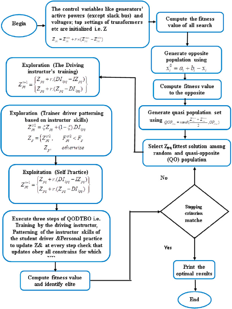
Figure 3. Flowchart for QODTBO.

$N_P$: population size,

m: number of independent variables.

$Z_{k,l}$ and $O{P}_{k,l}$ are $l^{th}$, respectively, independent variable of $k^{th}$ population vector Z and opposite population (OP).

Step 3: use the Newton–Raphson (NR) technique to achieve load flow (Pai, 1989) and evaluate entire dependent variables, for instance, active power for slack bus and load voltages.

Step 4: Determine the objective function’s value for Z and QOP.

Step 5: Choose the $N_P$ count of fittest members from Z and QOP based on computed objective function values.

Step 6: Contrasting the magnitude of the objective function, and get the driving instructor matrix $DI$.

Step 7: Opt a driving instructor in an arbitrary way from the $DI$ matrix.

Step 8: Using (Equation 49), get the $p^{th}$ DTBO member’s new position.

Step 9: Use the NR procedure to confirm whether or not the constraints are inside the bounds.

Step 10: Considering (Equation 50), the position of the $p^{th}$ DTBO member is updated. Patterning of the instructor skills of the student driver (Exploration)

Step 11: Use (Equation 53) to compute the patterning index.

Step 12: Appraise a fresh position of the $p^{th}$ DTBO component by (Equation 51).

Step 13: Verify whether the restrictions are within the bounds using the NR procedure.

Step 14: Use (Equation 52), to modify the $p^{th}$ DTBO member’s position. Personal practice (Exploitation)

Step 15: Determine the $p^{th}$ DTBO member’s new location using (Equation 54).

Step 16: Make sure whether the constraints are inside the bounds using the NR method.

Step 17: Use (Equation 55), to revise the situation of the $p^{th}$ DTBO constituent.

Step 18: On the basis of the jumping rate $J_r$ (probability based), following the creation of new populations Z using DTBO, the QOP is computed as described below. Then, the fitness value QOP is evaluated.

Step 19: Proceed to step 5 for the subsequent iteration until the terminating criterion is reached

Step 20: Output: The best candidate solution achieved by QODTBO

Algorithm 1

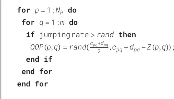
Algorithm 1.Opposite population based on the jumping rate.

5 Simulation results and comparisons for several cases

The following segment contains the simulation results of diverse OPF case studies applying the QODTBO technique with the pertinent analytical explanation. The MATLAB environment is being adopted for the entire simulations. IEEE 57 & 118 bus setups are being considered in this paper. The entire study can be broadly divided into four test scenarios. In each of them, there are four different objective functions. Table 1 provides the summaries of several test scenarios and their corresponding cases. The considered cost and emission factors for thermal generators are tabulated in Table 2. Parameters for distribution of wind flow and solar irradiance and power rating of wind and PV units with their cost coefficients are also provided in Table 2. Weibull-based wind speed PDF for scale factor 9 and shape factor 2 is shown in Figure 4A. Lognormal-based solar irradiance PDF is given in Figure 4B.

Figure 4

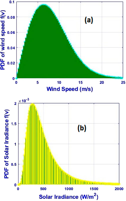
Figure 4. (A) Wind speed PDF; (B) solar irradiance PDF.

The coefficients of penalty and reserve cost are the same for wind and solar units. It should be noted that all the evaluated significant values of the various objective functions are noted in the provided Tables throughout the entire article for better visibility.

5.1 CEC benchmark system

The IEEE CEC benchmark system comprises a number of benchmark functions designed to evaluate the performance and behavior of various multi-objective combinatorial optimization tasks (MCTs). These functions are used to assess the MCT’s ability to explore different solutions, intensify toward optimum solutions, and converge successfully. The IEEE CEC benchmark system comes with 10D, 30D, 50D, and 100D dimensions as setup choices. In this study, however, we explicitly investigate the IEEE CEC 2017 benchmark system using 30D and 50D dimensions. In the IEEE CEC 2017 benchmark system, there are many functions that can be classified as unimodal, multi-modal, hybrid, or composite functions. The source of these functions is (Awad et al., 2017). Unimodal functions are used to assess the optimization process’s capacity to intensify toward a single optimal solution. Multi-modal functions evaluate the algorithm’s ability to investigate several solutions. Hybrid functions combine unimodal and multimodal properties. Composite functions are created by combining two or more unimodal and multimodal functions. For each experiment of the IEEE CEC benchmark systems, we set a maximum limit of function assessments as ${10}^4\times D$. The present authors evaluate the algorithm’s performance in 30 different runs. As mentioned earlier, there are several groups into which the test functions of the benchmark system under consideration may be separated: $F1-F3$, $F4-F16$, $F17-F22$, and $F23-F30$ are unimodal, multimodal, hybrid, and composite functions, respectively. As stated in (Awad et al., 2017), it is important to note that F2 is not included in the IEEE CEC 2017 benchmark system because of its unstable characteristics.

5.1.1 CEC 2017 (30D)

The best mean error values and standard deviations (SD) obtained by the proposed QODTBO and other MCTs for jointly unimodal and multimodal benchmark functions are shown statistically in Table 3 in the perspective of 30 dimensions (30D). Mean error values less than 10e-08 are considered to be 0 for all participating MCTs. Table 3 clearly shows that, in terms of mean error values, our proposed MCT outperforms most of the other cutting-edge MCTs utilized in this work for the majority of the test functions. In contrast to the other MCTs considered, the modifications we made to our proposed MCT have effectively increased its capacity for intensification and diversification, as evidenced by the enhanced performance in reaching optimal values for unimodal and multimodal test functions. Furthermore, it is evident from the SD values in Table 3 that out of all the MCTs considered, the proposed QODTBO has the highest level of precision. Table 4 compares the best mean error values and SD generated by different MCTs for hybrid and composite functions. The results in Table 4 show that the proposed QODTBO performs better in terms of mean error values and SD when compared to the other MCTs in the experiment, suggesting that it has the potential to provide very accurate and effective outcomes. The Wilcoxon signed-rank test with a significance threshold of 0.05 is used to compare the mean error values of the proposed MCT with the other MCTs for each test function in order to assess the statistical significance (Derrac et al., 2011). The competing MCTs are assigned “+,” “ = ,” and “-” signs based on their statistical performance versus the suggested QODTBO, as determined by the results of the signed-rank test. An MCT’s performance better, equal to, or worse than that of the recommended QODTBO is indicated by the “+“, “ = “, and “-” symbols, respectively. Making this distinction is crucial. Table 4 confirms the statistical robustness of the proposed QODTBO over its rivals, which shows that among the participating MCTs, the proposed MCT receives the most “+” signs. Moreover, the Friedman rank test (Derrac et al., 2011) is used to assess the proposed MCT’s overall statistical performance. Based on the Friedman rank, the proposed QODTBO ranks first among all MCTs considered.

Table 3

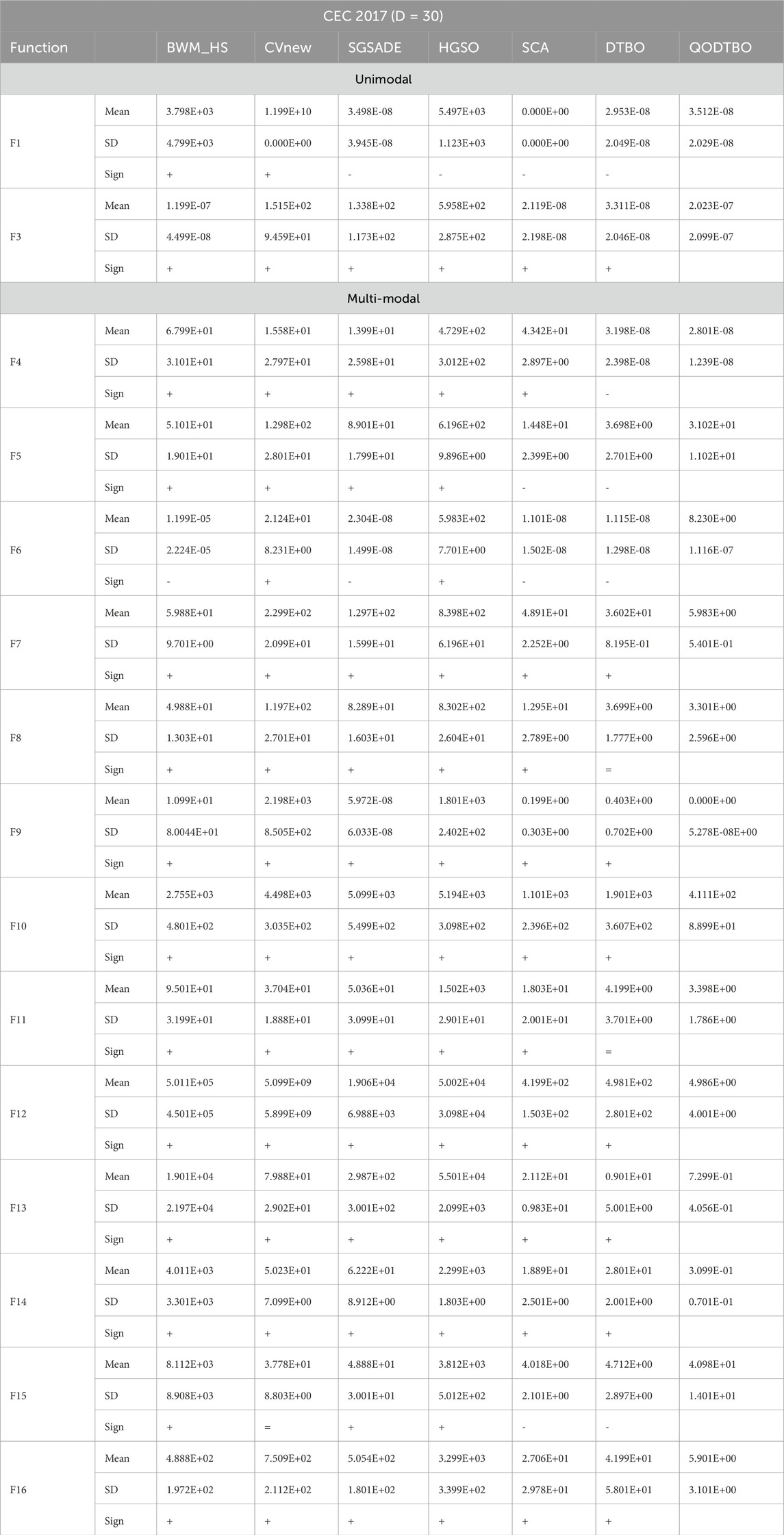
Table 3. Statistical comparison of QODTBO on CEC 2017 with 30D for $F1-F16$.

Table 4

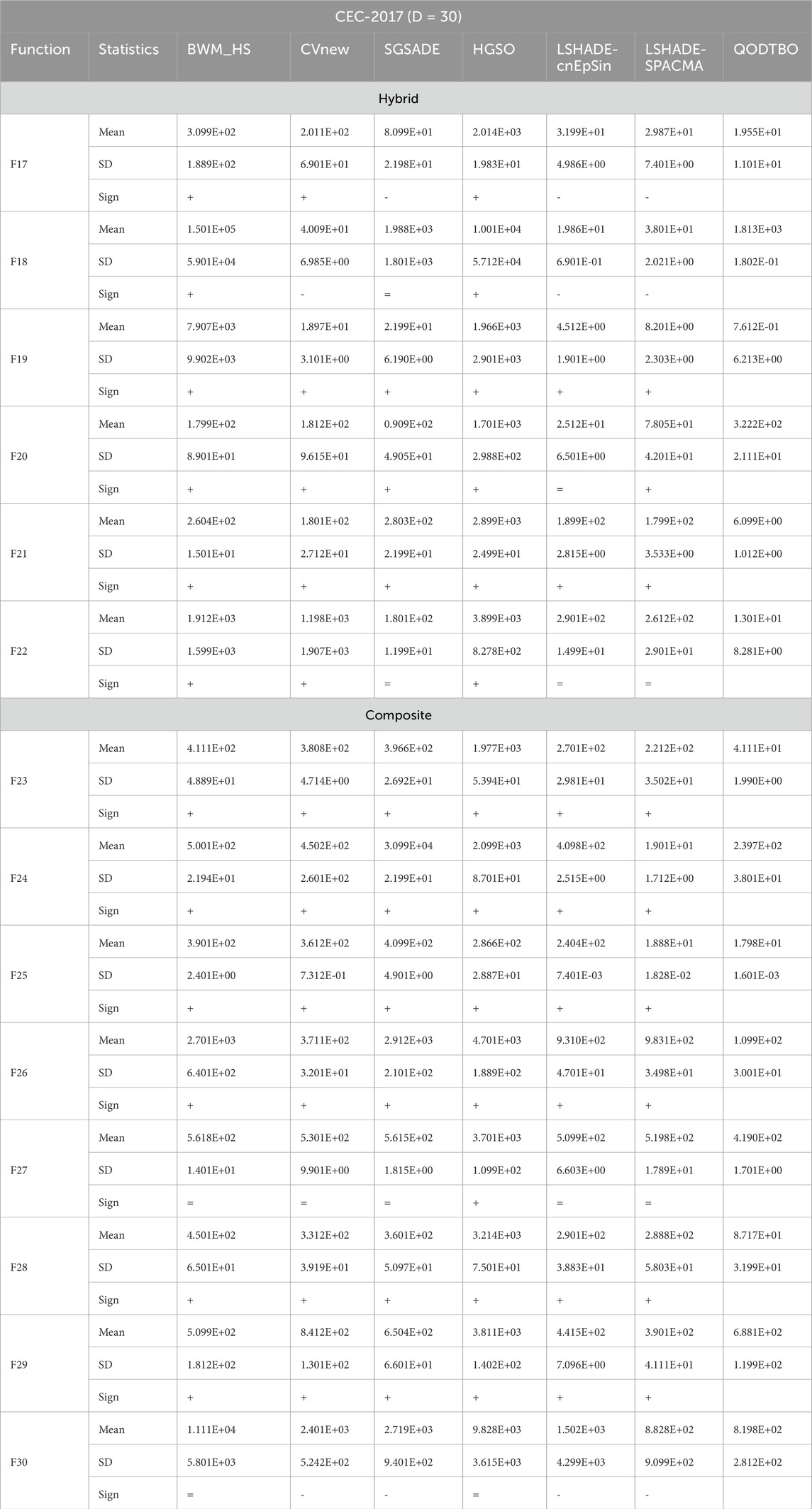
Table 4. Statistical comparison of QODTBO on CEC 2017 with 30D for $F17-F30$.

5.1.2 CEC 2017 (50D)

The best mean error values and standard deviations (SD) for the 50D scenario are shown in Table 4, which has been compiled by the suggested QODTBO and other participating MCTs. The competitiveness of the suggested QODTBO’s performance across most uni-modal and multi-modal functions is illustrated by the best mean error values displayed in Table 4. Additionally, the SD values show that the proposed strategy performs consistently better than the other strategies considered. According to Table 4, the recommended approach outperforms alternative approaches in terms of mean error values and SD for the majority of hybrid and composite functions. Since the proposed QODTBO receives more “+” signs than the other eligible MCTs, the results of the Wilcoxon signed-rank test, which are shown in Table 5, further substantiate its statistical superiority. Last but not least, the bottom row of Table 5 provides an unmistakable proof that, according to the Friedman rank test, the recommended QODTBO ranks first among all participating MCTs.

Table 5

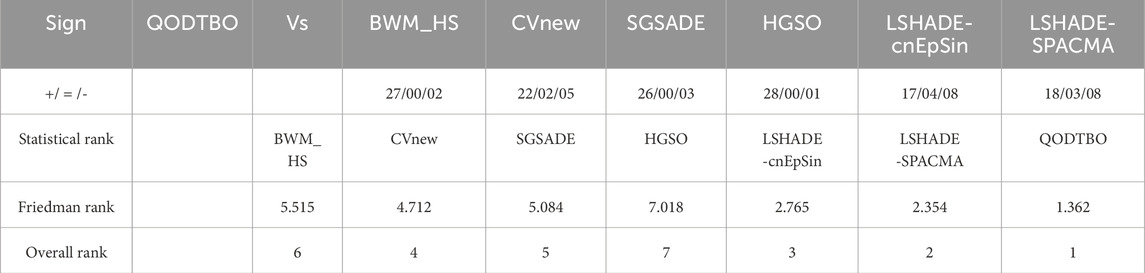
Table 5. The results of the Wilcoxon signed$-$rank test and Friedman rank test, considering the mean error value for CEC 2017 (D = 50).

5.2 Test scenario-1

Table 6 shows the overall system layout which is considered under test scenario-1. A similar system has been considered by Chaib et al. (2016) during their study where BSA had been employed. With the identical objectives as in Chaib et al. (2016), in the present work, in test scenario-1, the QODTBO algorithm has been proposed. From the obtained results, significant improvement in all considered cases has been noticed. The acquired results are displayed in Table 7.

Table 6

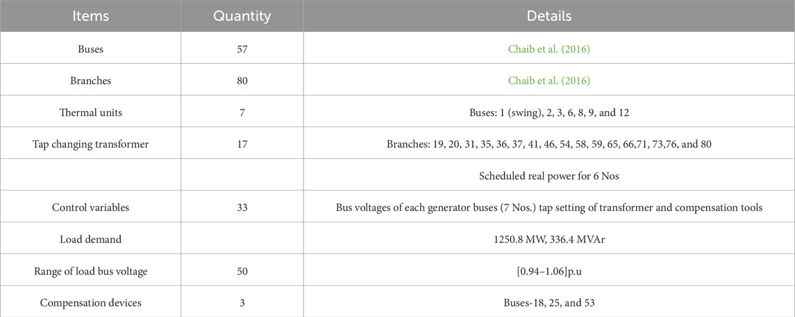
Table 6. An overview of the IEEE 57-bus setup at test scenario-1.

Table 7

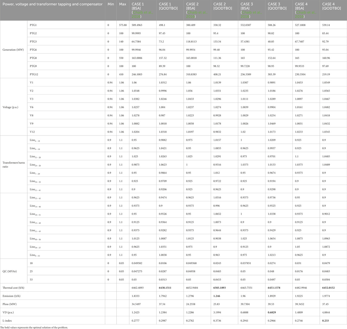
Table 7. Findings from simulations and the best control variable choices for Cases 1 through 4 (IEEE 57 bus test system).

In Table 7, results for case 1 to case 4 are observed. In case 1, it is found that the generation cost using QODTBO is 6430.1511 ($/h), whereas using BSA (Chaib et al., 2016), it was 6462.4093 ($/h). So the reduction in cost using QODTBO is 32.2582 ($/h) with respect to BSA. A comparative convergence curve among QODTBO, DTBO, and SCA for total cost reduction (case 1) is presented in Figure 5A which shows that QODTBO has accomplished improved results than DTBO and SCA. In case 2, where cost reduction and emission reduction are considered simultaneously, the use of QODTBO gave 6503.1893 ($/h) and 1.246(t/h), respectively. Both these quantities are superior to what was found by BSA (from Table 7). In case 3, reduction in cost and VD is considered simultaneously where the computed values are 6453.1378 ($/h) and 0.6829 (p.u.), respectively, using QODTBO (in Table 7) and are 6463.7551 ($/h) and 0.6888 (p.u), respectively, by BSA (Chaib et al., 2016). So it is observed that in case 3, the use of QODTBO provides a better outcome than BSA. The variations in bus voltages (in case 3) are depicted in Figure 6A. In test scenario 1, the aim of the last considered case (i.e., case 4) is to obtain minimum total cost and L-Index (a marker of voltage stability: the lower the index value, the higher the stability) at a time. In this case, the value of total cost and L-index is 6452.0152 ($/h) and 0.233, respectively, using QODTBO, whereas by BSA, their respective values are 6482.9946 ($/h) and 0.2746 (shown in Table 7). In addition, in this case, QODTBO performed better than BSA. In addition, test result statistical analysis has been conducted, and the statistical data are provided in Table 8. Based on these data, box plots are produced in Figures 7A–D, for Cases 1 to 4, respectively.

Figure 5

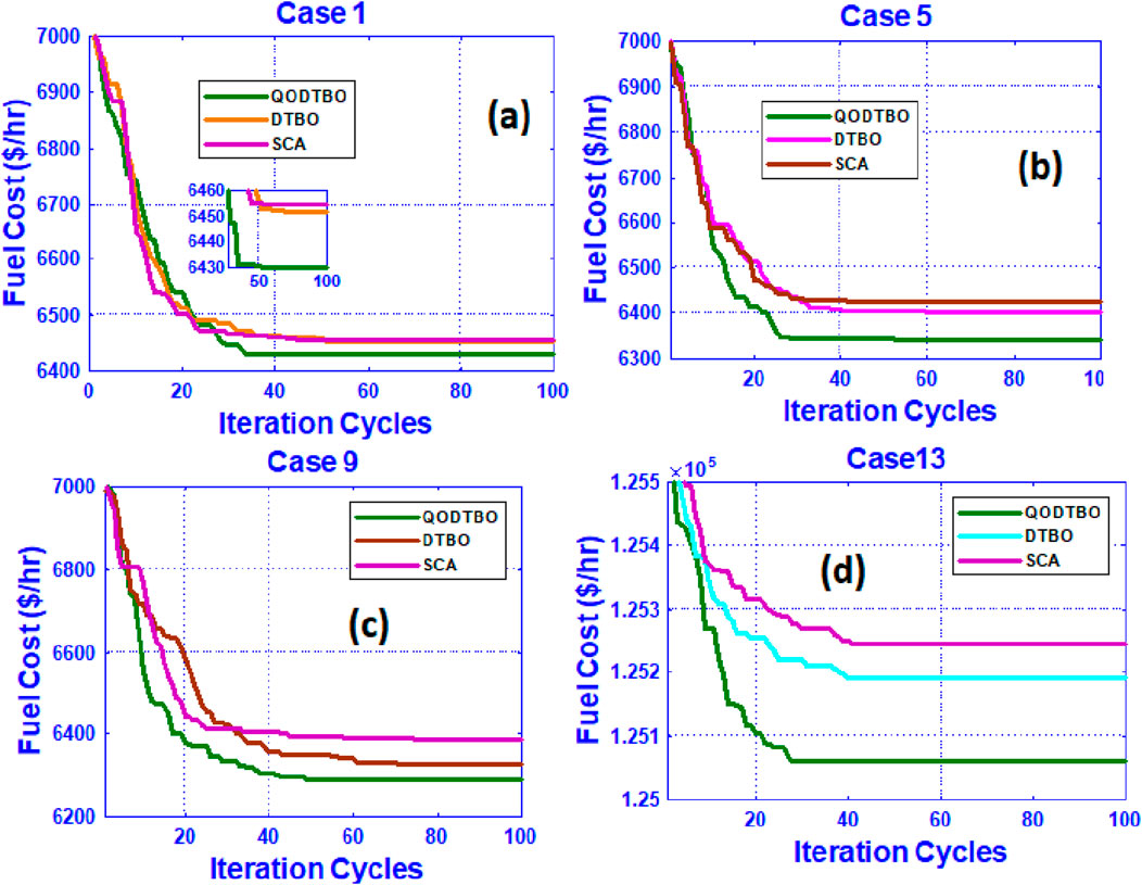
Figure 5. Convergence curves for (A) Case 1; (B) Case 5; (C) Case 9; and (D) Case 13.

Figure 6

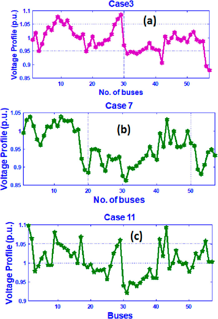
Figure 6. Bus voltage deviation for (A) Case 3; (B) Case 7; (C) Case 11.

Table 8

Table 8. Statistical assessment (30 trials) among different algorithms for the IEEE 57-bus system for cracking diverse cases.

Figure 7

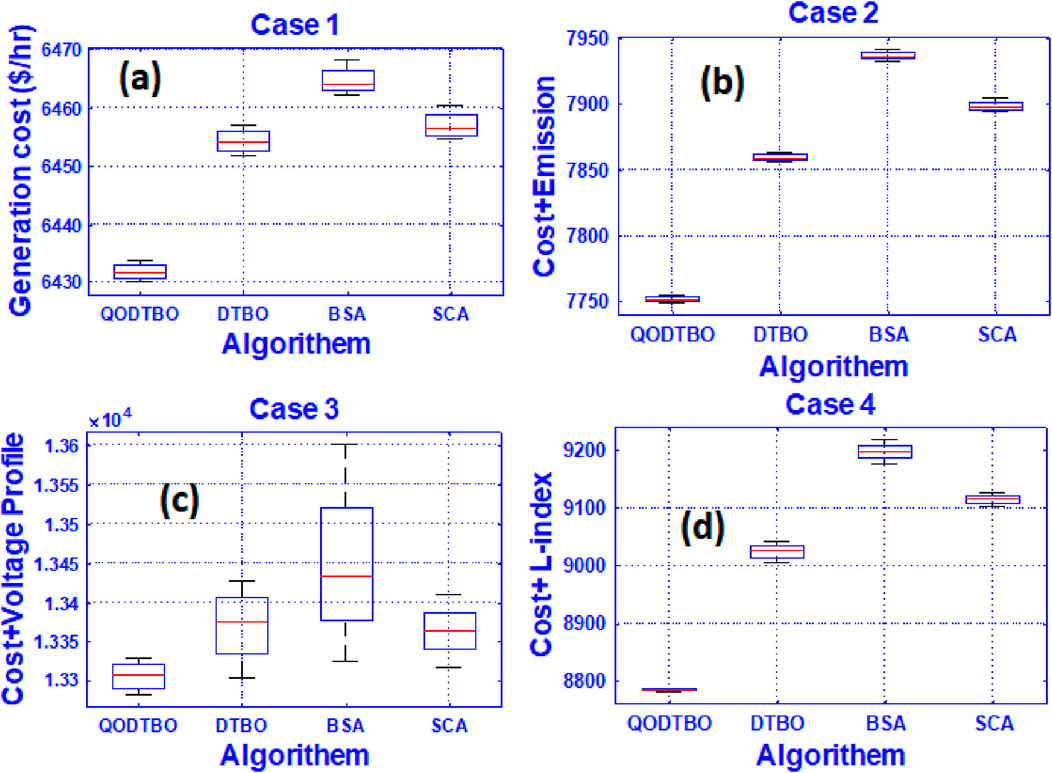
Figure 7. Box plots through QODTBO, DTBO, BSA, and SCA for (A) case 1; (B) Case 2; (C) Case 3; and (D) Case 4.

5.3 Test scenario-2

In test scenario-2, the considered test system is the revised IEEE 57 bus system where RESs (PV and wind unit) are incorporated with the test system which was adopted during test scenario-1 in this work. The summaries of this test network are provided in Table 6. In this test network, including single and multi-objective types, four different cases are studied like the cases considered in the last test scenario. Computed results for different cases (case 5 to case 8) are given in Table 9. Here, in case 5, lessening the total cost is the target. The computed value of the total price is 6342.393 ($/h). Results shown in Table 9 are obtained by QODTBO. It can be noticed that in the identical test network when RESs are included, the reduction in the overall cost is 87.7581 ($/h)[Comparing the obtained value in Table 6 and 9]. The value of the total cost (Case 5) that evolved with optimization iteration is displayed in Figure 5B, where the converging ability of QODTBO is compared with that of DTBO and SCA. In case 6, the goal is to diminish the overall cost and emissions together. The respective computed values are 6429.7488 ($/h) and 1.2014 (t/h). If these two values are compared with the values (6503.1893($/h) and 1.246(t/h)) found in case 2, test scenario 1, it can be said that the use of RESs has improved the objective function values. Case 7 and case 8 both are multi-objective problems, where the first one aims to simultaneously minimize total cost and VD and the second one intends to simultaneously reduce total cost and L-index. For case 7, obtained values are 6426.435 ($/h) and 0.6742 (p.u), respectively, while for case 8, the evaluated objective function values are 6399.1207 ($/h) and 0.2057, respectively. The voltage fluctuation (Case 7) over buses is shown in Figure 6B. If the results which are presented in Table 6 for case 3 and case 4 and the results displayed in Table 9 for case 7 and case 8 are being observed, it will again evidently reveal that the inclusion of RESs with IEEE 57 bus network enhances the whole performance. To compare the performances of QODTBO, DTBO and SCA, the statistical data are prepared upon 30 unbiased trials for each algorithm to carry out Case 5 to Case 8. The statistical records are produced in Table 8, and the box plots are placed in Figures 8A–D, for Case 5 to Case 8, respectively.

Table 9

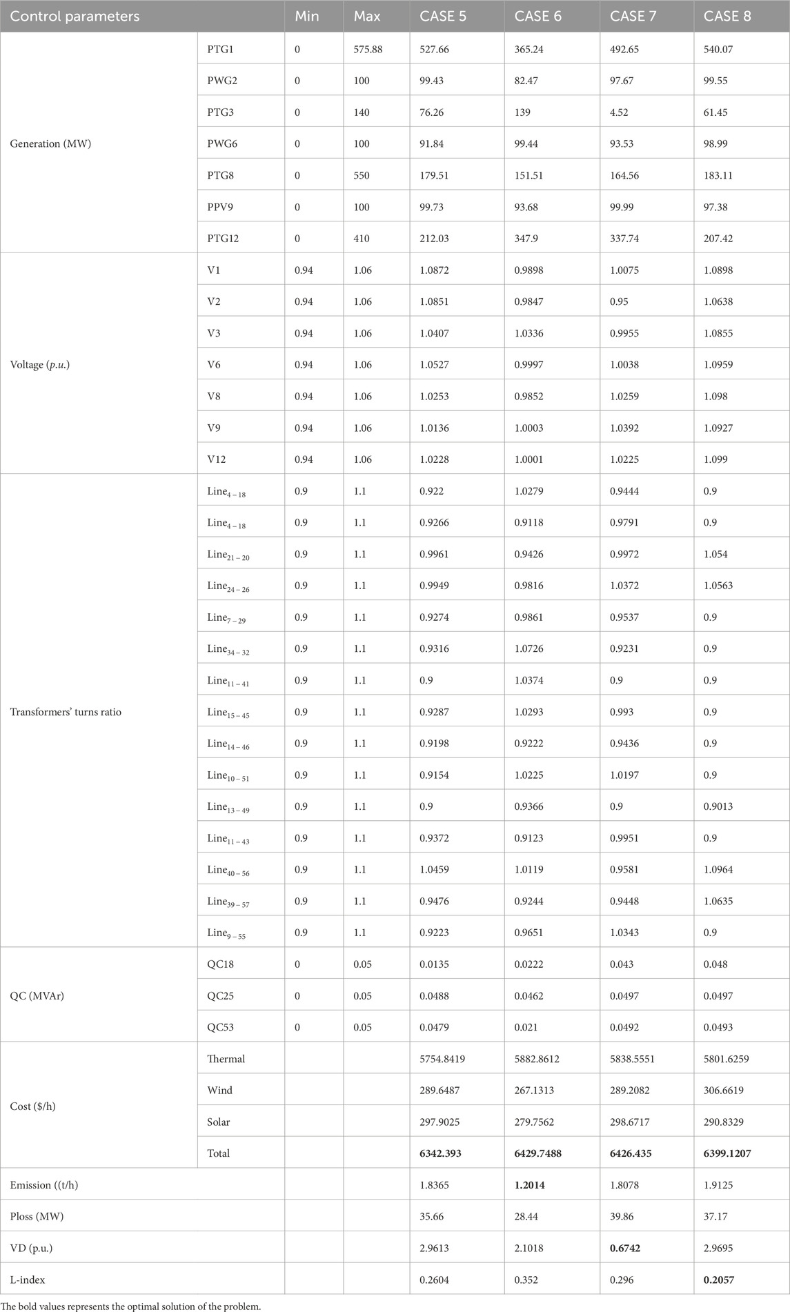
Table 9. Simulation findings and the best control variable settings for CASE 5 through CASE 8 (RESs included in the modified IEEE 57 bus test system).

Figure 8

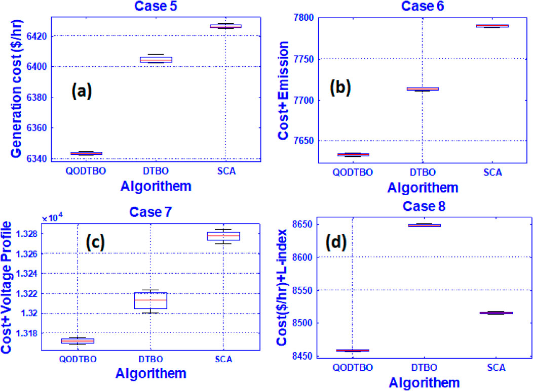
Figure 8. Box plots through QODTBO, DTBO, and SCA for (A) Case 5; (B) Case 6; (C) case 7; and (D) case 8.

5.4 Test scenario-3

In test scenario 3, the test system considered is similar to the immediate previous test network, but the only change is incorporating UPFC with it. The objective functions (through case 9 to case 12) that are taken care of in this test scenario are identical to the last two test scenarios. The quantities that are evaluated in this section are shown in Table 10. In case 9, where the goal is to obtain minimum total cost, the computed value is 6290.2794 ($/h). If case 1, case 5, and case 9 are looked at comparison, it is obvious that the overall cost is smallest in case 9, which signifies that the introduction of UPFC on the IEEE 57 bus system allied with RESs has improved the system performance. Figure 5C shows the curve of convergence for total cost (Case 9) minimization utilizing SCA, DTBO, and QODTBO. Case 10, case 11, and case 12 are designed to solve multi-objective functions as the last two test scenarios which are concurrently total cost and emission minimization, simultaneously total cost and VD reduction, and diminishing total cost and L-index at the same time, respectively. Obtained results for case 10 are 6392.5746($/h) and 1.1862 (t/h), respectively. For case 11, values of objective functions are 6304.6084($/h) and 0.6623 (p.u.), respectively. The deviation of bus voltages (in Case 11) are shown in Figure 6C. In case 12, the respective computed values are 6372.005 ($/h) and 0.2018. The important matter that has to be noticed is that for all considered objectives (it may be single or multi-objective), utilization of UPFC has upgraded all the test results.

Table 10

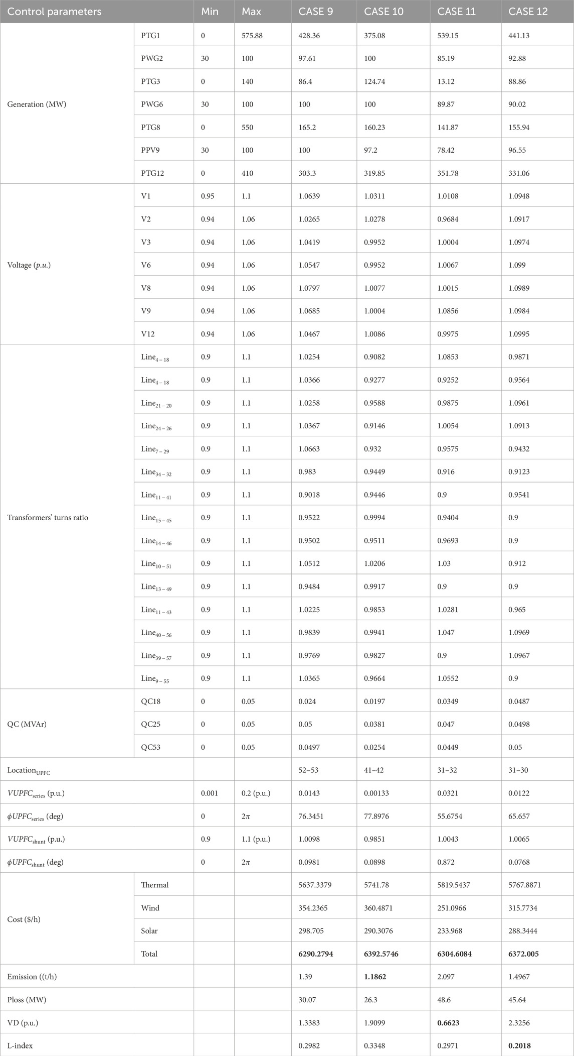
Table 10. Results of simulations and the best control variable settings were discovered for CASE 9 through CASE 12 (an adapted IEEE 57 bus test system with UPFC).

Table 8 is prepared to present a statistical measure over all the considered cases under the 57 bus network. These are computed using QODTBO, DTBO, BSA, and SCA, respectively. The statistical parameters which are concerned here are best (minimum), mean, median, and worst (maximum) values of the objective functions and standard deviation over 30 trials for case 9 to 12. The box plots over the statistical results for Case 9 to 12 are given in Figures 9A–D, respectively.

Figure 9

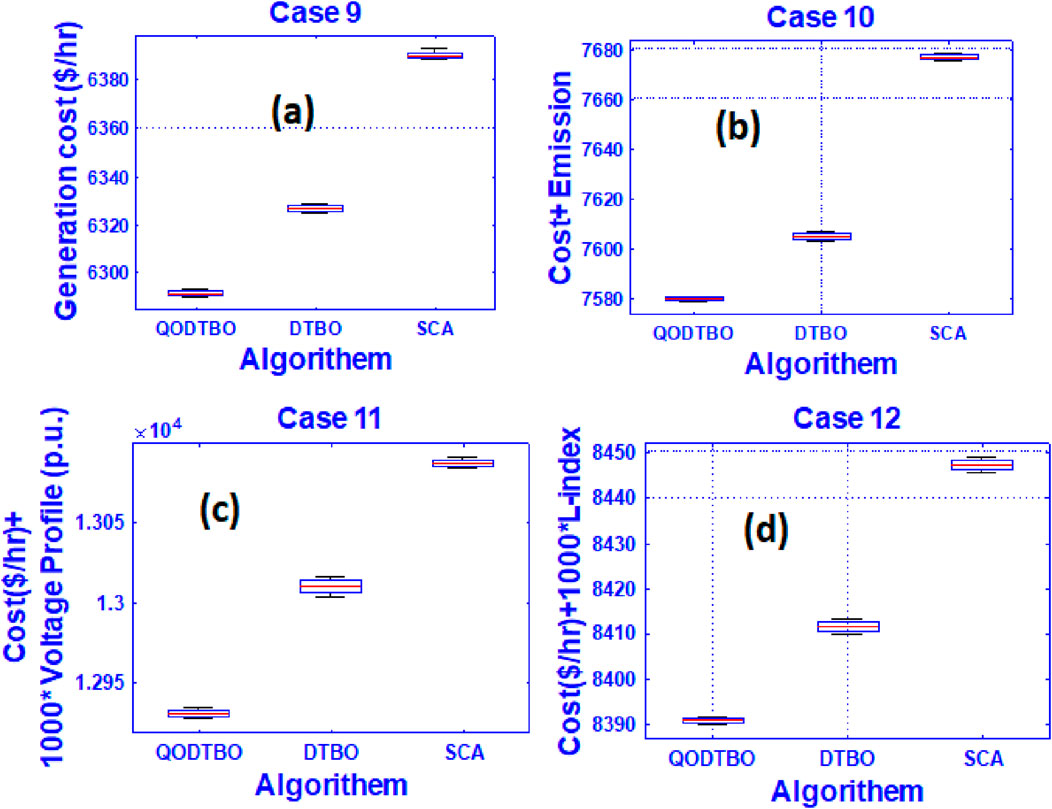
Figure 9. Box plots through QODTBO, DTBO, and SCA for (A) case 9; (B) case 10; (C) case 11; and (D) Case 12.

Finally, when a close look is placed on Table 8, the following important points are evident: (a) For all the considered cases (case 1–12), the obtained best (minimum) values of the total cost are lowest when QODTBO is used with respect to other optimization techniques. (b) Obtained standard deviations for all the cases with the help of QODTBO have been found to be minimum ones. Additionally, Table 8 shows the average number of function evaluations and average simulation time of 30 independent trials for case studies 1–12 in order to assess the effectiveness of the suggested method in terms of time and space complexity. The time and space complexity of the suggested QODTBO algorithm is clearly superior to those of other recently established DTBO and SCA algorithms, as indicated by the aforementioned time and space complexity related characteristics displayed in Table 8. Consequently, it can be said that, in terms of time and space complexity, the suggested QODTBO outperforms DTBO (Paul et al., 2024b) and BSA (Chaib et al., 2016). These pieces of evidence establish the fact that QODTBO is superior to other two optimization techniques (i.e., DTBO and BSA) and QODTBO is the most robust optimization scheme among optimization algorithms that are considered in this study.

5.5 Test scenario-4

At the last test scenario, the IEEE 118 bus system with RESs and UPFC is being opted for the experiment, which is briefed in Table 11. Moreover, to check the algorithm’s efficacy, cases 13–16 are taken care here. The outcomes are shown in Table 12. Based on obtained results, statistical data have been produced and displayed in Table 13 to contrast the potential of QODTBO, DTBO, and SCA algorithms to obtain the best OPF solution. Furthermore, in order to judge the efficacy of the proposed algorithm in terms of time and space complexity, the average number of function evaluation and average simulation time after 30 independent trials for cases 13–16 are illustrated in Table 13. The aforesaid time- and space complexity-related parameters shown in Table 13 clearly demonstrate that both time and space complexity of the proposed QODTBO algorithm are better than those of recently developed DTBO and SCA methods. Therefore, it can be concluded that the proposed QODTBO is the best fit among all suggested algorithms in terms of time and space complexity. The convergence diagrams for case 13 obtained by QODTBO, DTBO, and SCA algorithms are illustrated in Figure 5D. It is evident from this Table that QODTBO is the most robust, accurate, and reliable tool in solving the OPF issue among the considered algorithms. To make the statistical results more trustworthy, the one-way ANOVA test has been carried out for cases 13 and 14 whose outcomes are given in Tables 14 and 15 and on Figures 10A,B respectively. For cases 15 & Case 16, the error-bar plots are placed in Figures 10C,D, respectively.

Table 11

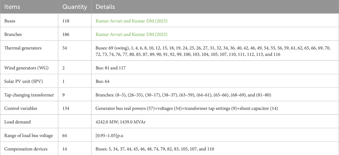
Table 11. An overview of IEEE 118- bus System under study.

Table 12

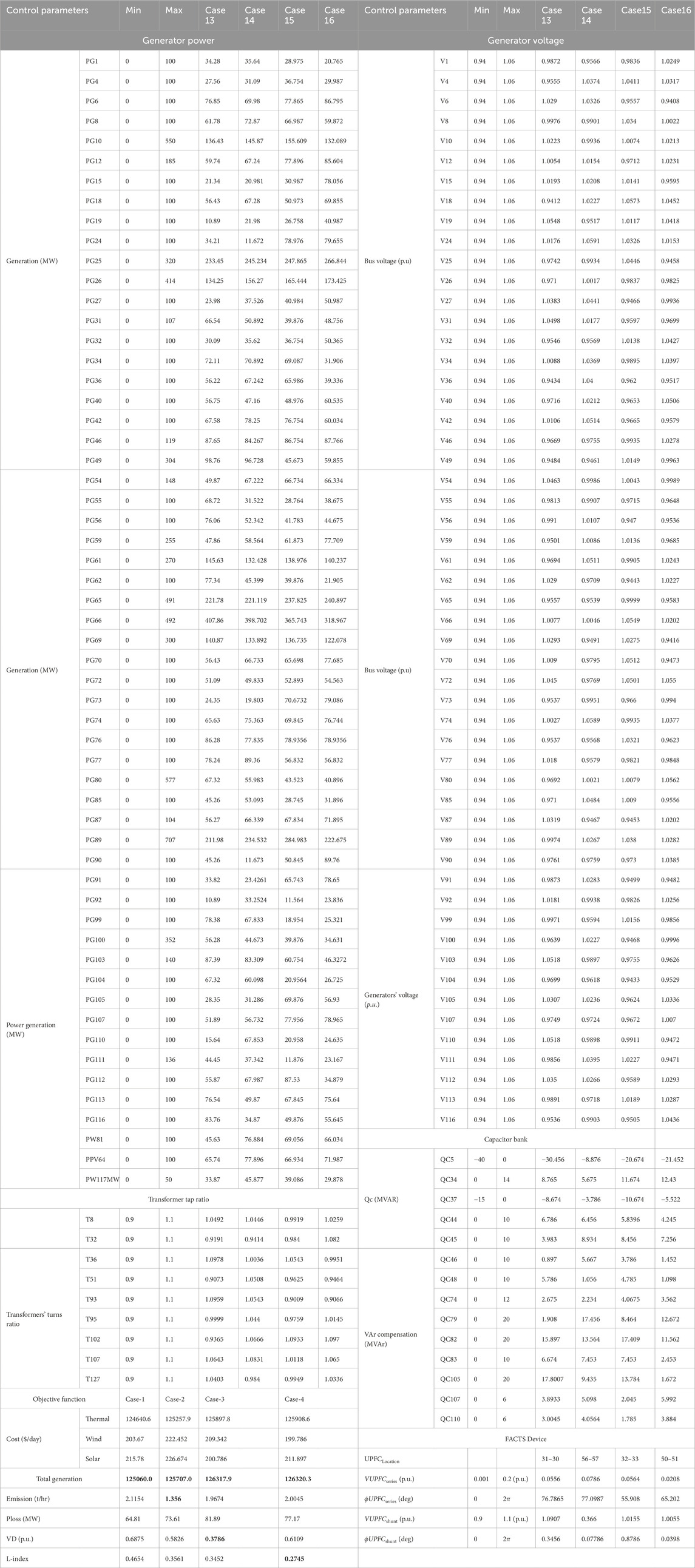
Table 12. Simulation results of case studies with fixed loading (100%) with FACTs for the adapted IEEE 118 bus system.

Table 13

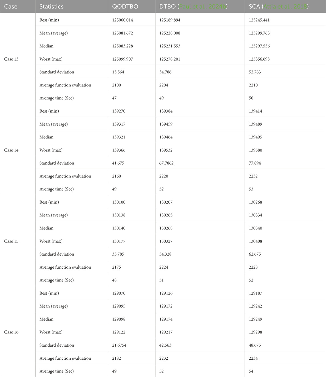
Table 13. Statistical comparison (30 trials) among various algorithms for the IEEE 118 bus system for solving different cases.

Table 14

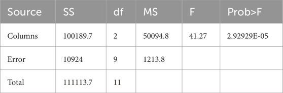
Table 14. ANOVA result for Case 13.

Table 15

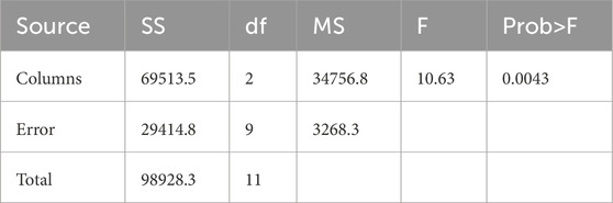
Table 15. ANOVA result for Case 14.

Figure 10

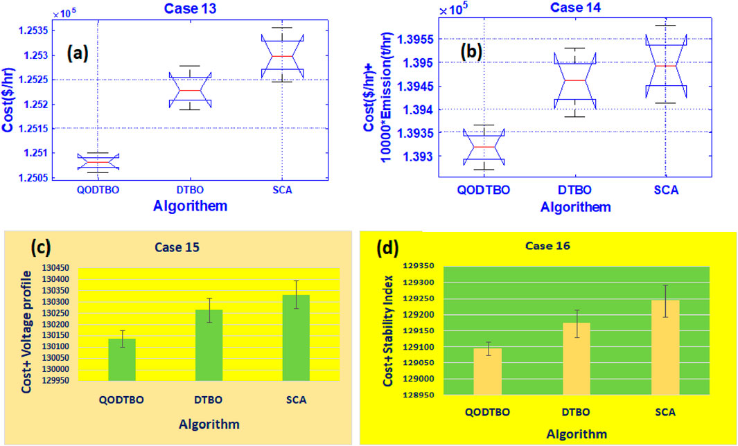
Figure 10. (A) Case 13: ANOVA result; (B) Case 14: ANOVA result; (C) error bar diagram for Case 15; and (D) error bar diagram for Case 16.

6 Conclusion and future scope

In this study, the QODTBO scheme has been employed to explore OPF solutions for the IEEE 57 & 118 bus test system. The considered four different test setups are as follows: at the beginning traditional IEEE 57 bus system, then IEEE 57 bus network with RESs, IEEE 57 bus network with RESs and UPFC, and finally IEEE 118 bus system having RESs and UPFC are accesses. For these entire test scenarios, there is one single-objective function and three multi-objective functions. Achieving minimum generation cost, simultaneously obtaining minimum generation cost and emission, simultaneously accomplishing minimum generation cost and VD, and attaining minimum generation cost and voltage stability index at a time are being chosen as single- and multi-objective functions, respectively. The results that have been evaluated by QODTBO are compared with the results found using DTBO, BSA, and SCA. It is observed that in every considered case for every test setup, QODTBO outperforms DTBO, BSA, and SCA. From statistical measures of the test results, it is understood that QODTBO is the most robust technique among the stated optimization tools used in this paper. Another significant observation is that, when RESs are incorporated with the traditional IEEE 57 bus system, the performance of the system has been enhanced, and while RESs and UPFC both are being introduced with the traditional IEEE 57 bus network, the performance has been further enriched. The performance of QODTBO is tested on higher IEEE bus systems ($i.e$ 118 bus system), and the effectiveness and superiority of QODTBO are again established from the experimental outcomes. The statistical analysis accompanied with one-way ANOVA test firmly assures the fact that QODTBO has a better performance among other considered algorithms. The experiments can be re-performed with the advent of more efficient new optimization techniques in the future.Consequently, the proposed approach effectively manages the large and complex power system, which may inspire future researchers to use the QODTBO algorithm in other contexts.

• The proposed system can be expanded to include more sources in order to assess the QODTBO optimization’s superiority.

•By incorporating additional, more complex renewable energy sources into the suggested system, the dynamic ability of the QODTBO algorithm can be evaluated.

•By combining machine learning and evolutionary techniques, the proposed QODTBO algorithm can be extended in a real-time practical power system.

Data availability statement

The raw data supporting the conclusions of this article will be made available by the authors, without undue reservation.

Author contributions

TS: writing – original draft, writing – review and editing. CP: writing – original draft, writing – review and editing. SD: writing – original draft, writing – review and editing. PR: writing – original draft, writing – review and editing. GT: writing – original draft, writing – review and editing. SM: writing – original draft, writing – review and editing.

Funding

The author(s) declare that no financial support was received for the research and/or publication of this article.

Conflict of interest

The authors declare that the research was conducted in the absence of any commercial or financial relationships that could be construed as a potential conflict of interest.

Generative AI statement

The author(s) declare that no Gen AI was used in the creation of this manuscript.

Publisher’s note

All claims expressed in this article are solely those of the authors and do not necessarily represent those of their affiliated organizations, or those of the publisher, the editors and the reviewers. Any product that may be evaluated in this article, or claim that may be made by its manufacturer, is not guaranteed or endorsed by the publisher.

References

Abdollahi, A., Ali, A. G., Miveh, M. R., Mohammadi, F., and Jurado, F. (2020). Optimal power flow incorporating facts devices and stochastic wind power generation using krill herd algorithm. Electronics 9 (6), 1043. doi:10.3390/electronics9061043

CrossRef Full Text | Google Scholar

Abdullah, M., Javaid, N., Khan, I. U., Ali Khan, Z., Chand, A., and Ahmad, N. (2020). “Optimal power flow with uncertain renewable energy sources using flower pollination algorithm,” in Advanced information networking and applications: proceedings of the 33rd international conference on advanced information networking and applications (AINA-2019) 33 (Springer), 95–107.

Google Scholar

Adhikari, A., Jurado, F., Naetiladdanon, S., Sangswang, A., Kamel, S., and Ebeed, M. (2023). Stochastic optimal power flow analysis of power system with renewable energy sources using adaptive lightning attachment procedure optimizer. Int. J. Electr. Power and Energy Syst. 153, 109314. doi:10.1016/j.ijepes.2023.109314

CrossRef Full Text | Google Scholar

Aghaebrahimi, M. R., Golkhandan, R. K., and Ahmadnia, S. (2016). “Localization and sizing of facts devices for optimal power flow in a system consisting wind power using hbmo,” in 2016 18th mediterranean electrotechnical conference (MELECON) (IEEE), 1–7.

CrossRef Full Text | Google Scholar

Alasali, F., Nusair, K., Obeidat, A. M., Foudeh, H., and Holderbaum, W. (2021). An analysis of optimal power flow strategies for a power network incorporating stochastic renewable energy resources. Int. Trans. Electr. Energy Syst. 31 (11), e13060. doi:10.1002/2050-7038.13060

CrossRef Full Text | Google Scholar

Ali, S. A. (2022). A hybrid firefly–jaya algorithm for the optimal power flow problem considering wind and solar power generations. Appl. Sci. 12 (14), 7193. doi:10.3390/app12147193

CrossRef Full Text | Google Scholar

Ali Mohamed, A.-A., Mohamed, Y. S., El-Gaafary, A. A. M., and Hemeida, A. M. (2017). Optimal power flow using moth swarm algorithm. Electr. Power Syst. Res. 142, 190–206. doi:10.1016/j.epsr.2016.09.025

CrossRef Full Text | Google Scholar

Amal, A. M., Kamel, S., Hassan, M. H., Mosaad, M. I., and Aljohani, M. (2022). Optimal power flow analysis based on hybrid gradient-based optimizer with moth–flame optimization algorithm considering optimal placement and sizing of facts/wind power. Mathematics 10 (3), 361. doi:10.3390/math10030361

CrossRef Full Text | Google Scholar

Annapandi, P., Banumathi, R., Pratheeba, N. S., and Manuela, A. A. (2021). RETRACTED: an efficient optimal power flow management based microgrid in hybrid renewable energy system using hybrid technique. Trans. Inst. Meas. Control 43 (1), 248–264. doi:10.1177/0142331220961687

CrossRef Full Text | Google Scholar

Attia, A.-F., El Sehiemy, R. A., and Hasanien, H. M. (2018). Optimal power flow solution in power systems using a novel sine-cosine algorithm. Int. J. Electr. Power and Energy Syst. 99, 331–343. doi:10.1016/j.ijepes.2018.01.024

CrossRef Full Text | Google Scholar

Awad, N. H., Ali, M. Z., and Suganthan, P. N. (2017). Problem definitions and evaluation criteria for the cec 2017 special session and competition on single objective real-parameter numerical optimization. Changsha: National University of Defense Technology. Hunan, PR China and Kyungpook National University.

Google Scholar

Bakirtzis, A. G., Biskas, P. N., Zoumas, C. E., and Petridis, V. (2002). Optimal power flow by enhanced genetic algorithm. IEEE Trans. Power Syst. 17 (2), 229–236. doi:10.1109/tpwrs.2002.1007886

CrossRef Full Text | Google Scholar

Ben Attous, D., and Labbi, Y. (2009). “Particle swarm optimization based optimal power flow for units with non-smooth fuel cost functions,” in 2009 international conference on electrical and electronics engineering - eleco 2009, I–377–I–381.

Google Scholar

Bentouati, B., Chettih, S., El Sehiemy, R., and Wang, G. (2017). Elephant herding optimization for solving non-convex optimal power flow problem. J. Electr. Electron. Eng. 10 (1), 31.

Google Scholar

Biswas, P. P., Arora, P., Mallipeddi, R., Suganthan, P. N., and Panigrahi, B. K. (2021). Optimal placement and sizing of facts devices for optimal power flow in a wind power integrated electrical network. Neural Comput. Appl. 33, 6753–6774. doi:10.1007/s00521-020-05453-x

CrossRef Full Text | Google Scholar

Biswas, P. P., Suganthan, P. N., Mallipeddi, R., and Amaratunga, G. A. J. (2018a). Optimal power flow solutions using differential evolution algorithm integrated with effective constraint handling techniques. Eng. Appl. Artif. Intell. 68, 81–100. doi:10.1016/j.engappai.2017.10.019

CrossRef Full Text | Google Scholar

Biswas, P. P., Suganthan, P. N., Mallipeddi, R., and Amaratunga, G. A. J. (2018b). Optimal power flow solutions using differential evolution algorithm integrated with effective constraint handling techniques. Eng. Appl. Artif. Intell. 68, 81–100. doi:10.1016/j.engappai.2017.10.019

CrossRef Full Text | Google Scholar

Bouchekara, H. R. E. H., Chaib, A. E., Abido, M. A., and El-Sehiemy, R. A. (2016). Optimal power flow using an improved colliding bodies optimization algorithm. Appl. Soft Comput. 42, 119–131. doi:10.1016/j.asoc.2016.01.041

CrossRef Full Text | Google Scholar

Burchett, R. C., Happ, H. H., and Vierath, D. R. (1984). Quadratically convergent optimal power flow. IEEE Trans. Power Apparatus Syst. PAS-103, 3267–3275. doi:10.1109/tpas.1984.318568

CrossRef Full Text | Google Scholar

Chaib, A. E., Bouchekara, H. R. E. H., Mehasni, R., and Abido, M. A. (2016). Optimal power flow with emission and non-smooth cost functions using backtracking search optimization algorithm. Int. J. Electr. Power and Energy Syst. 81, 64–77. doi:10.1016/j.ijepes.2016.02.004

CrossRef Full Text | Google Scholar

Dai, L., Xiao, H., and Yang, P. (2024). Robust optimal power flow considering uncertainty in wind power probability distribution. Front. Energy Res. 12, 1402155. doi:10.3389/fenrg.2024.1402155

CrossRef Full Text | Google Scholar

Daqaq, F., Ouassaid, M., Kamel, S., Ellaia, R., and El-Naggar, M. F. (2022). A novel chaotic flower pollination algorithm for function optimization and constrained optimal power flow considering renewable energy sources. Front. Energy Res. 10, 941705. doi:10.3389/fenrg.2022.941705

CrossRef Full Text | Google Scholar

Dehghani, M., Trojovská, E., and Trojovskỳ, P. (2022). A new human-based metaheuristic algorithm for solving optimization problems on the base of simulation of driving training process. Sci. Rep. 12 (1), 9924. doi:10.1038/s41598-022-14225-7

PubMed Abstract | CrossRef Full Text | Google Scholar

Derrac, J., García, S., Molina, D., and Herrera, F. (2011). A practical tutorial on the use of nonparametric statistical tests as a methodology for comparing evolutionary and swarm intelligence algorithms. Swarm Evol. Comput. 1 (1), 3–18. doi:10.1016/j.swevo.2011.02.002

CrossRef Full Text | Google Scholar

Devaraj, D., and Yegnanarayana, B. (2005). Genetic-algorithm-based optimal power flow for security enhancement. IEE Proceedings-Generation, Transm. Distribution 152 (6), 899–905. doi:10.1049/ip-gtd:20045234

CrossRef Full Text | Google Scholar

Duman, S., Jie, L, and Wu, L. (2021). Ac optimal power flow with thermal–wind–solar–tidal systems using the symbiotic organisms search algorithm. IET Renew. Power Gener. 15 (2), 278–296. doi:10.1049/rpg2.12023

CrossRef Full Text | Google Scholar

Duman, S., Li, J., Wu, L., and Guvenc, U. (2020). Optimal power flow with stochastic wind power and facts devices: a modified hybrid psogsa with chaotic maps approach. Neural Comput. Appl. 32, 8463–8492. doi:10.1007/s00521-019-04338-y

CrossRef Full Text | Google Scholar

Dutta, S., Roy, P. K., and Nandi, D. (2015). Optimal location of upfc controller in transmission network using hybrid chemical reaction optimization algorithm. Int. J. Electr. Power and Energy Syst. 64, 194–211. doi:10.1016/j.ijepes.2014.07.038

CrossRef Full Text | Google Scholar

Ebeed, M., Kamel, S., and Jurado, F. (2018). “Optimal power flow using recent optimization techniques,” in Classical and recent aspects of power system optimization (Elsevier), 157–183.

CrossRef Full Text | Google Scholar

Elattar, E. E., and ElSayed, S. K. (2019). Modified jaya algorithm for optimal power flow incorporating renewable energy sources considering the cost, emission, power loss and voltage profile improvement. Energy 178, 598–609. doi:10.1016/j.energy.2019.04.159

CrossRef Full Text | Google Scholar

Farhat, M., Kamel, S., Atallah, A. M., and Khan, B. (2021). Optimal power flow solution based on jellyfish search optimization considering uncertainty of renewable energy sources. IEEE Access 9, 100911–100933. doi:10.1109/access.2021.3097006

CrossRef Full Text | Google Scholar

Guvenc, U., Duman, S., Tolga Kahraman, H., Aras, S., and Katı, M. (2021). Fitness–distance balance based adaptive guided differential evolution algorithm for security-constrained optimal power flow problem incorporating renewable energy sources. Appl. Soft Comput. 108, 107421. doi:10.1016/j.asoc.2021.107421

CrossRef Full Text | Google Scholar

Gyugyi, L. (1992). Unified power-flow control concept for flexible ac transmission systems. IET generation, transmission and distribution, 139 (4), 323–331.

CrossRef Full Text | Google Scholar

Hamid, R. T. (2005). “Opposition-based learning: a new scheme for machine intelligence,” in International conference on computational intelligence for modelling, control and automation and international conference on intelligent agents, web technologies and internet commerce CIMCA-IAWTIC’06 (IEEE), 1, 695–701.

Google Scholar

Hassan, M. H., Kamel, S., Alateeq, A., Alassaf, A., and Alsaleh, I. (2023). Optimal power flow analysis with renewable energy resource uncertainty: a hybrid aeo-co approach. IEEE Access 11, 122926–122961. doi:10.1109/access.2023.3328958

CrossRef Full Text | Google Scholar

Hassan, M. H., Kamel, S., Alateeq, A., Alassaf, A., and Alsaleh, I. (2024). Optimal power flow in hybrid wind-pv-v2g systems with dynamic load demand using a hybrid mrfo-aha algorithm. IEEE Access 12, 174297–174329. doi:10.1109/access.2024.3496123

CrossRef Full Text | Google Scholar

Herwan Sulaiman, M., and Mustaffa, Z. (2021). Solving optimal power flow problem with stochastic wind–solar–small hydro power using barnacles mating optimizer. Control Eng. Pract. 106, 104672. doi:10.1016/j.conengprac.2020.104672

CrossRef Full Text | Google Scholar

Hoang Bao Huy, T., Nguyen, T. P., Nor, N. M., Elamvazuthi, I., Ibrahim, T., and Vo, D. N. (2022). Performance improvement of multiobjective optimal power flow-based renewable energy sources using intelligent algorithm. IEEE Access 10, 48379–48404. doi:10.1109/access.2022.3170547

CrossRef Full Text | Google Scholar

Jamal, R., Zhang, J., Men, B., Habib Khan, N., Mohamed, E., Jamal, T., et al. (2024). Chaotic-quasi-oppositional-phasor based multi populations gorilla troop optimizer for optimal power flow solution. Energy 301, 131684. doi:10.1016/j.energy.2024.131684

CrossRef Full Text | Google Scholar

Jangir, P., Agrawal, S. P., Pandya, S. B., Parmar, A., Kumar, S., Tejani, G. G., et al. (2025). A cooperative strategy-based differential evolution algorithm for robust pem fuel cell parameter estimation. Ionics 31 (1), 703–741. doi:10.1007/s11581-024-05963-x

CrossRef Full Text | Google Scholar

Jangir, P., Ezugwu, A. E., Arpita, S. P. A., Pandya, S. B., Parmar, A., Gulothungan, G., et al. (2024a). Precision parameter estimation in proton exchange membrane fuel cells using depth information enhanced differential evolution. Sci. Rep. 14 (1), 29591. doi:10.1038/s41598-024-81160-0

PubMed Abstract | CrossRef Full Text | Google Scholar

Jangir, P., Ezugwu, A. E., Saleem, K., Arpita, S. P. A., Pandya, S. B., Parmar, A., et al. (2024b). A hybrid mutational northern goshawk and elite opposition learning artificial rabbits optimizer for pemfc parameter estimation. Sci. Rep. 14 (1), 28657. doi:10.1038/s41598-024-80073-2

PubMed Abstract | CrossRef Full Text | Google Scholar

Jangir, P., Ezugwu, A. E., Saleem, K., Arpita, S. P. A., Pandya, S. B., Parmar, A., et al. (2024c). A levy chaotic horizontal vertical crossover based artificial hummingbird algorithm for precise pemfc parameter estimation. Sci. Rep. 14 (1), 29597. doi:10.1038/s41598-024-81168-6

PubMed Abstract | CrossRef Full Text | Google Scholar

Kaymaz, E., Duman, S., and Guvenc, U. (2021). Optimal power flow solution with stochastic wind power using the Lévy coyote optimization algorithm. Neural Comput. Appl. 33, 6775–6804. doi:10.1007/s00521-020-05455-9

CrossRef Full Text | Google Scholar

Kessel, P., and Glavitsch, H. (1986). Estimating the voltage stability of a power system. IEEE Trans. power Deliv. 1 (3), 346–354. doi:10.1109/tpwrd.1986.4308013

CrossRef Full Text | Google Scholar

Khamees, A. K., Abdelaziz, A. Y., Eskaros, M. R., Attia, M. A., and Sameh, M. A. (2023). Optimal power flow with stochastic renewable energy using three mixture component distribution functions. Sustainability 15 (1), 334. doi:10.3390/su15010334

CrossRef Full Text | Google Scholar

Kumar Avvari, R., and Kumar Dm, V. (2023). A new hybrid evolutionary algorithm for multi-objective optimal power flow in an integrated we, pv, and pev power system. Electr. Power Syst. Res. 214, 108870. doi:10.1016/j.epsr.2022.108870

CrossRef Full Text | Google Scholar

Kumar Avvari, R., and Vinod Kumar, D. M. (2022). Multi-objective optimal power flow including wind and solar generation uncertainty using new hybrid evolutionary algorithm with efficient constraint handling method. Int. Trans. Electr. Energy Syst., 2022.

Google Scholar

Maheshwari, A., Sood, Y. R., and Jaiswal, S. (2022). Investigation of optimal power flow solution techniques considering stochastic renewable energy sources: review and analysis. Wind Eng., 0309524X221124000.

Google Scholar

Mandal, B., and Roy, P. K. (2014). Multi-objective optimal power flow using quasi-oppositional teaching learning based optimization. Appl. soft Comput. 21, 590–606. doi:10.1016/j.asoc.2014.04.010

CrossRef Full Text | Google Scholar

Moeini-Aghtaie, M., Ali, A., Fotuhi-Firuzabad, M., and Hajipour, E. (2014). A decomposed solution to multiple-energy carriers optimal power flow. IEEE Trans. Power Syst. 29 (2), 707–716. doi:10.1109/tpwrs.2013.2283259

CrossRef Full Text | Google Scholar

Mohamed, A. M. S., Hasanien, H. M., and Al-Durra, A. (2021). Solving of optimal power flow problem including renewable energy resources using heap optimization algorithm. IEEE Access 9, 35846–35863. doi:10.1109/access.2021.3059665

CrossRef Full Text | Google Scholar

Mohamed, E., Mostafa, A., Aly, M. M., Jurado, F., and Kamel, S. (2023). Stochastic optimal power flow analysis of power systems with wind/pv/tcsc using a developed Runge kutta optimizer. Int. J. Electr. Power and Energy Syst. 152, 109250. doi:10.1016/j.ijepes.2023.109250

CrossRef Full Text | Google Scholar

Mosbah, M., Zine, R., Arif, S., Mohammedi, R. D., and Bacha, S. (2018). “Optimal power flow for transmission system with photovoltaic based dg using biogeography-based optimization,” in 2018 international conference on electrical sciences and technologies in maghreb (CISTEM) (IEEE), 1–6.

CrossRef Full Text | Google Scholar

Nagarajan, K., Rajagopalan, A., Bajaj, M., Raju, V., and Blazek, V. (2025). Enhanced wombat optimization algorithm for multi-objective optimal power flow in renewable energy and electric vehicle integrated systems. Results Eng. 25, 103671. doi:10.1016/j.rineng.2024.103671

CrossRef Full Text | Google Scholar

Nusair, K., Alasali, F., Ali, H., and Holderbaum, W. (2021). Optimal placement of facts devices and power-flow solutions for a power network system integrated with stochastic renewable energy resources using new metaheuristic optimization techniques. Int. J. Energy Res. 45 (13), 18786–18809. doi:10.1002/er.6997

CrossRef Full Text | Google Scholar

Nusair, K., and Alhmoud, L. (2020). Application of equilibrium optimizer algorithm for optimal power flow with high penetration of renewable energy. Energies 13 (22), 6066. doi:10.3390/en13226066

CrossRef Full Text | Google Scholar

Olofsson, M., Andersson, G., and Soder, L. (1995). Linear programming based optimal power flow using second order sensitivities. IEEE Trans. power Syst. 10 (3), 1691–1697. doi:10.1109/59.466472

CrossRef Full Text | Google Scholar

Pai, A. (1989). Energy function analysis for power system stability. Springer Science and Business Media.

Google Scholar

Panda, A., Tripathy, M., Barisal, A. K., and Prakash, T. (2017). A modified bacteria foraging based optimal power flow framework for hydro-thermal-wind generation system in the presence of statcom. Energy 124, 720–740. doi:10.1016/j.energy.2017.02.090

CrossRef Full Text | Google Scholar

Pandya, S. B., and Jariwala, H. R. (2020). Renewable energy resources integrated multi-objective optimal power flow using non-dominated sort grey wolf optimizer. J. Green Eng. 10 (1), 180–205.

Google Scholar

Papi Naidu, T., Venkateswararao, B., and Balasubramanian, G. (2021). “Whale optimization algorithm based optimal power flow: in view of power losses, voltage stability and emission,” in 2021 innovations in power and advanced computing technologies (i-PACT), 1–6.

Google Scholar

Paul, C., Sarkar, T., Dutta, S., and Roy, P. K. (2024a). Multi-objective combined heat and power with wind–solar–ev of optimal power flow using hybrid evolutionary approach. Electr. Eng. 106 (2), 1619–1653. doi:10.1007/s00202-023-02171-0

CrossRef Full Text | Google Scholar

Paul, C., Sarkar, T., Dutta, S., and Roy, P. K. (2024b). Integration of optimal power flow with combined heat and power dispatch of renewable wind energy based power system using chaotic driving training based optimization. Renew. Energy Focus 49, 100573. doi:10.1016/j.ref.2024.100573

CrossRef Full Text | Google Scholar

Radman, G., and Raje, R. S. (2007). Power flow model/calculation for power systems with multiple facts controllers. Electr. power Syst. Res. 77 (12), 1521–1531. doi:10.1016/j.epsr.2006.10.008

CrossRef Full Text | Google Scholar

Rambabu, M., Kumar, G. V. N., and Sivanagaraju, S. (2019). Optimal power flow of integrated renewable energy system using a thyristor controlled seriescompensator and a grey-wolf algorithm. Energies 12 (11), 2215. doi:10.3390/en12112215

CrossRef Full Text | Google Scholar

Riaz, M., Hanif, A., Hussain, S. J., Memon, M. I., Ali, M. U., and Zafar, A. (2021). An optimization-based strategy for solving optimal power flow problems in a power system integrated with stochastic solar and wind power energy. Appl. Sci. 11 (15), 6883. doi:10.3390/app11156883

CrossRef Full Text | Google Scholar

Roy, P., and Mandal, D. (2012). Quasi-oppositional biogeography-based optimization for multi-objective optimal power flow. Electr. Power Components Syst. 40, 236–256. doi:10.1080/15325008.2011.629337

CrossRef Full Text | Google Scholar

Roy, P. K., Mandal, B., and Bhattacharya, K. (2012). Gravitational search algorithm based optimal reactive power dispatch for voltage stability enhancement. Electr. Power Components Syst. 40 (9), 956–976. doi:10.1080/15325008.2012.675405

CrossRef Full Text | Google Scholar

Shaheen, M. A. M., Hasanien, H. M., Turky, R. A., Ćalasan, M., Zobaa, A. F., and Aleem, S. H. E. A. (2021). Opf of modern power systems comprising renewable energy sources using improved chgs optimization algorithm. Energies 14 (21), 6962. doi:10.3390/en14216962

CrossRef Full Text | Google Scholar

Shaheen, M. A. M., Ullah, Z., Qais, M. H., Hasanien, H. M., Chua, K. J., Tostado-Véliz, M., et al. (2022). Solution of probabilistic optimal power flow incorporating renewable energy uncertainty using a novel circle search algorithm. Energies 15 (21), 8303. doi:10.3390/en15218303

CrossRef Full Text | Google Scholar

Shilaja, C. (2021). “Perspective of combining chaotic particle swarm optimizer and gravitational search algorithm based on optimal power flow in wind renewable energy,” in Soft computing techniques and applications: proceeding of the international conference on computing and communication. IC3 2020 (Springer), 477–490.

Google Scholar

Siavash, M., Pfeifer, C., Rahiminejad, A., and Vahidi, B. (2017a). “An application of grey wolf optimizer for optimal power flow of wind integrated power systems,” in 2017 18th international scientific conference on electric power engineering (EPE) (IEEE), 1–6.

CrossRef Full Text | Google Scholar

Siavash, M., Pfeifer, C., Rahiminejad, A., and Vahidi, B. (2017b). “An application of grey wolf optimizer for optimal power flow of wind integrated power systems,” in 2017 18th international scientific conference on electric power engineering (EPE), 1–6.

Google Scholar

Sun, D. I., Ashley, B., Brewer, B., Hughes, A., and Tinney, W. F. (1984). Optimal power flow by Newton approach. IEEE Trans. Power Apparatus Syst. 130 (10), 2864–2880. doi:10.1109/tpas.1984.318284

CrossRef Full Text | Google Scholar

Surender Reddy, S. (2017). Multi-objective optimal power flow for a thermal-wind-solar power system. J. Green Eng. 7 (4), 451–476. doi:10.13052/jge1904-4720.741

CrossRef Full Text | Google Scholar

Ullah, Z., Wang, S., Radosavljević, J., and Lai, J. (2019). A solution to the optimal power flow problem considering wt and pv generation. IEEE Access 7, 46763–46772. doi:10.1109/access.2019.2909561

CrossRef Full Text | Google Scholar

Ullah Khan, I., Javaid, N., Gamage, K. A. A., James Taylor, C., Baig, S., and Ma, X. (2020). Heuristic algorithm based optimal power flow model incorporating stochastic renewable energy sources. IEEE Access 8, 148622–148643. doi:10.1109/access.2020.3015473

CrossRef Full Text | Google Scholar

Warid, W., Hizam, H., Mariun, N., and Wahab, N. I. A. (2018). A novel quasi-oppositional modified jaya algorithm for multi-objective optimal power flow solution. Appl. Soft Comput. 65, 360–373. doi:10.1016/j.asoc.2018.01.039

CrossRef Full Text | Google Scholar

Xu, Q., Wang, L., Wang, N, Hei, X., and Zhao, L (2014). A review of opposition-based learning from 2005 to 2012. Eng. Appl. Artif. Intell. 29, 1–12. doi:10.1016/j.engappai.2013.12.004

CrossRef Full Text | Google Scholar

Yan, X., and Quintana, V. H. (1999). Improving an interior-point-based opf by dynamic adjustments of step sizes and tolerances. IEEE Trans. Power Syst. 14 (2), 709–717. doi:10.1109/59.761902

CrossRef Full Text | Google Scholar

Zhang, S., and Irving, M. R. (1994). Enhanced Newton-Raphson algorithm for normal, controlled and optimal powerflow solutions using column exchange techniques. IEE Proceedings-Generation, Transm. Distribution 141 (6), 647–657. doi:10.1049/ip-gtd:19941479

CrossRef Full Text | Google Scholar

Zhang, W., Peng, Z., Wang, Q., Qi, W., and Ge, Y. (2024). Optimal power flow method with consideration of uncertainty sources of renewable energy and demand response. Front. Energy Res. 12, 1421277. doi:10.3389/fenrg.2024.1421277

CrossRef Full Text | Google Scholar