Monitoring modeling and analysis of the electromagnetic environment of HVDC transmission lines based on ion flow and wind coupling field

High-voltage direct current transmission lines are an integral part of the power system, but the ion flow field and total electric field they generate can be harmful. Moreover, two of the most critical indicators for evaluating environmental compatibility, ion current density ρ_j and total electric field strength E, can be affected by wind. The difficulty in monitoring and modeling the ion flow and wind coupling field has caused recent research to consider only transverse winds and not take into account the wind directions. As a result, it cannot model the actual situation accurately for monitoring and analysis. For this reason, this article takes the ±800 kV Jinsu Line in Huzhou as an example and constructs a 3-D monitoring model using the finite element method. The nonlinear mapping relationship between the model design parameters and the feature parameters is approximated by an extreme learning machine, and the actual measurement results are used to invert the model design parameters to modify the finite element model and realize the precise monitoring of the ρ_j and E in different wind speed and direction situations. The results show that the modified model can realize the condition monitoring of the electromagnetic environment of transmission lines with an improved accuracy of 20.86%. In addition, some laws are discovered: the peak absolute values of ρ_j and E increase and then decrease with the increase in wind speed; at low wind speed, the smaller the included angle between the wind direction and the line direction is, the smaller the peaks are; at high wind speed, the smaller the included angle is, the peaks increase and then decrease.

1 Introduction

A transmission line is a critical part of the power system. The development of high-voltage direct current (HVDC) transmission lines realizes the macro-control of energy and conforms to the development trend of power grids (Zhang et al., 2007). However, when a corona occurs in an HVDC transmission line, the ions formed by ionization move toward the nearby space under the action of the electric field force, forming an ion flow (Cui et al., 2012), and the superposition of the ion flow field with the nominal electric field of the line creates a total electric field, which causes electromagnetic hazards (Zou et al., 2017). The ion flow intercepted per unit area on the ground is called the ion current density ρ_j, and the strength of the total electric field at the ground level is called E. Both ρ_j and E are the most important evaluation indicators of the electromagnetic environment, which determine the limitations of the transmitted power and operating voltage of the power system (Zou et al., 2020). As the demand for electricity in the power system increases, power grid companies must balance the efficiency of energy delivery and environmental compatibility, and the monitoring and analysis of ρ_j and E have become major issues in ensuring the safety and reliability of the power system during transmission and distribution (Chen, 2014).

Scholars have conducted extensive research to address this issue. In terms of on-site monitoring, Wen et al. (1985) laid the foundation for systematic monitoring of the ion current density using a current probe with a microcurrent amplifier. Zhang et al. (2009) and Wang and Chen (2015) expanded and optimized the monitoring methods and analyzed the results and environmental impacts. In terms of digital monitoring, Janischewskyj and Cela (1979) proposed the use of finite element numerical modeling to refine the positive and negative ion composite problem in ion flow simulations. Lu et al. (2008) and Li et al. (2012) optimized the solution efficiency and accuracy. Lu et al. (2014) and Yang et al. (2015) synthesized tests and simulations to verify the feasibility of the software model for transmission line condition monitoring. Park et al. (2018) and Zou et al. (2023) proposed various improvement methods, such as the flux tracing method and BPA FEM, respectively. Bai et al. (2023) and Wan (2023) performed ion flow monitoring for typical scenarios versus high-altitude scenarios for HVDC lines, respectively, and made specifications for conductor selection.

However, it is difficult to further minimize the error due to natural factors, especially the effect of wind on ion flow (Lu et al., 2010). In the past few years, some scholars have investigated the effect of transverse wind on ρ_j and E (Qiao et al., 2019; Wu, 2019). Xu et al. (2020) constructed a model for monitoring the ion flow field at low wind speeds. Choopum and Techaumnat (2022), Yi et al. (2022), and Lin (2024) studied the trend of change. Du et al. (2022) optimized monitoring in high-altitude situations. The monitoring accuracy of the upflow finite element method under windy conditions is gradually improving (Cai et al., 2023), and Xu et al. (2023) and Qi et al. (2024a) applied the method to construct ion flow monitoring for complex multi-conductor systems. Kang et al. (2024) used the fluid equation to further explore the accuracy of the monitoring model. However, in practical engineering, natural wind does not always come from a single direction. The previous researchers attributed the wind bias problem of ion flow to the study of the effect of wind speed on it, while ignoring the wind blowing from different directions, which makes the existing monitoring models less accurate in areas where the distribution of wind direction is more dispersed and lacks the analysis of trend studies incorporating wind direction.

If we want to consider the natural wind in different directions, there must be a 3-D monitoring modeling of the ion flow-wind field, and the determination of some model design parameters is more complex and difficult. The large 3-D spatial field and the extremely small radius of the line conductors make the difference of finite element mesh size large, and the mesh dissecting and connecting is more difficult, which has a certain nonlinear effect on the results. Fortunately, the extreme learning machine (Huang et al., 2006; Huang et al., 2012) based on a feed-forward neural network can map this nonlinear relationship efficiently and accurately, so it can be applied to modify the finite element model.

Based on this, this article proposes a modeling method for electromagnetic environment monitoring of transmission lines considering the effect of wind on ion flow field with different wind speeds and directions, taking the case of the ±800 kV Jinsu Line in Huzhou, China, as an example. Then, a mesh optimization method is proposed to approximate the nonlinear mapping relationship between model design parameters and feature parameters by training an extreme learning machine neural network through the initial model, and then the model design parameters are obtained by back-calculating to modify the finite element model using the actual measurement results. The accurate condition monitoring and characterization study of ρ_j and E considering both the influence of wind speed and direction are finally realized. The article provides engineering guidance for electromagnetic environment monitoring of HVDC transmission lines and steady operation of power systems.

2 Initial monitoring model

2.1 Control equations

We start by constructing an initial 3-D finite element model. When constructing a wind field to satisfy the practical situation, the wind gradient must be considered first, and the wind shear equation must be introduced. The wind speed increases with the height from the ground, and a simplified wind shear function for the near-ground side is given by Cai et al. (2023):

$W=W_0{\left(\frac{h}{H_0}\right)}^{0.3},(1)$

where W₀ is the wind speed at the reference point; H₀ is the height of the reference point, generally taken as 10 m; and W is the wind speed at the height h from the ground.

A three-dimensional wind field capable of considering different wind directions should satisfy

$\mathbf{W}=W\cos \left(\theta \right)\mathbf{i}+W\sin \left(\theta \right)\mathbf{j},(2)$

where θ is the wind direction, W is the wind vector, i is the unit vector in the horizontal direction, and j is the unit vector in the vertical direction.

The ion flow field of the transmission line is subsequently coupled in the wind field, and the following simplifications are made:

(1) The thickness of the ionized layer is negligibly small.

(2) The ion mobility is constant and independent of the electric field strength.

(3) The influence of the spatial diffusion of ions is neglected.

From the Poisson equation, we can obtain

${\nabla }^2\varphi =-\frac{{\rho }^{+}-{\rho }^{-}}{{\epsilon }_0},(3)$

where φ is the electric potential of the total electric field; ρ⁺ and ρ⁻ are the positive and negative electric charge densities, respectively; and ε₀ is the vacuum dielectric constant.

The ion flow is blown by the vector wind to migrate and satisfy the following equation:

${\mathbf{j}}^{+}={\rho }^{+}\left(k^{+}\mathbf{E}+\mathbf{W}\right),(4)$

${\mathbf{j}}^{-}={\rho }^{-}\left(k^{-}\mathbf{E}-\mathbf{W}\right),(5)$

$\mathbf{E}=-\nabla \varphi ,(6)$

where j⁺ and j⁻ are the densities of positive and negative ions, respectively; k⁺ and k⁻ are the mobilities of positive and negative ions, respectively; and E is the electric field strength.

The transportation equation of electric charge is

$\nabla ·{\mathbf{j}}^{+}=-\frac{R_{ion}}{e}{\rho }^{+}{\rho }^{-},(7)$

$\nabla ·{\mathbf{j}}^{-}=\frac{R_{ion}}{e}{\rho }^{+}{\rho }^{-},(8)$

where R_ion is the recombination coefficient of the ions and e is the electron charge.

2.2 Boundary delimitation and boundary conditions

The solution area and boundary delineation of the finite element model are shown in Figure 1, where the air domain is divided into the near-line area A and the other area B. Different mesh parameters are used for the different mesh dissections. We make some preliminary settings for the finite element mesh. The mesh of the 3-D field needs to use the free tetrahedral mesh as the basic cell because this mesh is the easiest to use in dealing with the boundaries of large and small cells; second, it is necessary to smooth the control entities across the removal. The number of iterations is chosen to be 4, and the maximal depth of the cell to be dealt with is 4, so the quality of the grid cells is guaranteed. Then, certain lower-quality cells are allowed to be received during the grid generation to improve construction efficiency, but attention should be paid to avoiding too-large or too-small cells, and inverted bending cells are not allowed to appear. Finally, the curvature factor of the whole finite element mesh model is taken as 0.3, and the resolution of the narrow region is taken as 0.85, so that the geometrical approximation of the mesh is more accurate, and the narrow region will not lose the key geometrical features or lead to the computational error due to the overly rough mesh.

Figure 1

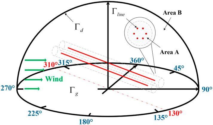
Figure 1. Boundary delimitation.

The electric potential φ satisfies Equation 9:

$\phi =\left\{\begin{array}{l}{U}_{line},\left(x,y,z\right)\in {\mathrm{\Gamma }}_{line},\\ 0,\left(x,y,z\right)\in {\mathrm{\Gamma }}_g,\\ U_{csm},\left(x,y,z\right)\in {\mathrm{\Gamma }}_{\mathrm{d}},\end{array}\right.(9)$

where Γ_line, Γ_g, and Γ_d are the artificial boundaries of the line surface, ground, and air domains, respectively; U_line is the line operating voltage; and U_csm is the potential at the artificial boundary, which can be calculated by the simulated electric charge method, and the electric charge density at the place should be approximated as zero.

The calculation satisfies Kaptzov’s assumption (Tadasu et al., 1981) that the surface electric field strength of the wire is always maintained at the strength at which the corona occurs, as Equation 10 shows.

$\left|\mathbf{E}·\mathbf{n}\right|=E_o,\left(x,y,z\right)\in {\mathrm{\Gamma }}_{line},(10)$

where n is the unit outward normal vector on the surface of the wire and E₀ is the field strength at which the corona occurs, which can be calculated by Peek’s formula and is usually taken as 18 kV/cm (Cai et al., 2023).

For HVDC transmission lines, it can be assumed that the initial electric charge density ρ on the surface of the wire is similar to that of a concentric cylindrical structure (Lu et al., 2007), and the relationship between the electric charge density and the electric field is (Xu et al., 2023), as Equations 11, 12 shows.

$U_0=E_{0}r\ln \frac{H}{r},(11)$

$\rho =\left\{\begin{array}{l}\frac{4{\epsilon }_0{U}_0{E}_g\left(U_{line}-U_0\right)}{rH{E}_0{U}_{line}\left(5-\frac{4U_0}{U_{line}}\right)}\\ 0,E_{NRM}<E_0,\end{array}\right.,E_{NRM}\ge E_0,(12)$

where U₀ is the voltage that the corona occurs; E_g is the maximum nominal electric field strength at the ground location; r is the radius of the wire; and H is the height of the line. Furthermore, E_NRM is the nominal electric field strength of the surface of the wire; if the value is greater than the E₀, there is an electric charge density on the surface of the wire; otherwise, the wire does not generate a corona, and the electric charge density is 0.

2.3 Convergence criteria

This is a forward calculation process according to Poisson’s equation to calculate the potential and electric field strength at each point. Then, solving the current continuity equation to get the new space charge density at each point by using the potential and electric field strength at each point is a reverse calculation process. Every completion of a forward and reverse calculation is considered an iteration. The new charge density is used to solve Poisson’s equation to get the new potential and electric field strength. Then, the new potential and electric field strength are substituted to get the new space charge density until the electric field strength and space charge density on the surface of the conductor meet the results of the calculation of the error requirements of X, Y; that is the end of the iteration. When the error requirements are not met, the wire surface charge density is corrected according to the calculated electric field strength value, and the iterative solution is repeated after the correction. The error requirements are given by Equations 13, 14, and the correction formula is given by Equation 15.

${\delta }_E=\frac{\left|E_{\max }-E_C\right|}{E_C}<0.5\%,(13)$

${\delta }_p=\frac{\left|{\rho }_n-{\rho }_{n-1}\right|}{{\rho }_{n-1}}<0.1\%,(14)$

${\rho }_{s}n={\rho }_s\left(n-1\right)\left[1+\mu \frac{E_{\max }-E_C}{E_{\max }+E_C}\right],(15)$

where E_C is the halo field strength; E_max is the maximum field strength at the wire surface; δ_E and δ_ρ are the relative error of the field strength at the wire surface and the relative error of the space charge density, respectively; ρ_sn, ρ_s(n−1) are the values of the surface charge density of the wire in the n th and n−1st iterations, respectively; ρ_n, ρ_n−1 are the values of the space charge density after the nth and n−1st iteration, respectively; and μ > 0 is the correction factor, which is taken as 2 in this article.

3 Model modification

3.1 Principles of modification

Mesh generation for finite element model design requires manually setting different mesh parameters followed by automatic dissections while satisfying Delaunay properties. Low-quality meshes have nonlinear effects on the simulation results. The mesh-design parameter modification is an inverse problem belonging to the finite element computation. The modification requires multiple attempts in the mesh design of the finite element model, which is more time-consuming and laborious and is prone to fall into a local optimal solution in the case of large errors.

In order to avoid a large number of iterations and complex nonlinear optimization calculations, we take the mesh-design parameter x as the dependent variable and the feature parameter y as the independent variable and use the extreme learning machine (ELM) neural network to solve the mapping function (Di et al., 2022). The ELM neural network can transform the model modification problem into a positive problem, which can be expressed in the form of an inverse function as Equation 16.

$x=f^{-1}\left(y\right).(16)$

We randomly select n sets of initial mesh-design parameters x₀ and substitute them into the initial finite element model to obtain n sets of feature parameters y₀, which are used as the sample set. The sample set is allocated as a training set and validation set according to a certain ratio. We use the training set to train the ELM neural network to get the mapping relationship. The validation set is substituted into f⁻¹ to calculate the coefficient of determination R². If R² > 0.99, the accuracy of the ELM neural network mapping can be verified. The formula of R² is as Equation 17.

$R^2=1-\frac{{{\displaystyle \sum }}_{i=1}^n{\left(x_i-{\widehat{x}}_i\right)}^2}{{{\displaystyle \sum }}_{i=1}^n{\left(x_i-\overline{x}\right)}^2},(17)$

where x_i is the initial mesh-design parameter of the ith sample, ${\widehat{x}}_i$ is the ELM output value of the i th sample, and $\overline{x}$ is the average value of all x_i.

The true values of the feature parameters y_m are obtained through practical tests, and the modified mesh-design parameters x_m can be obtained by substituting f⁻¹, which can be used for accurate modeling. In summary, the general flow of the finite element model modification method based on the ELM neural network is shown in Figure 2.

Figure 2

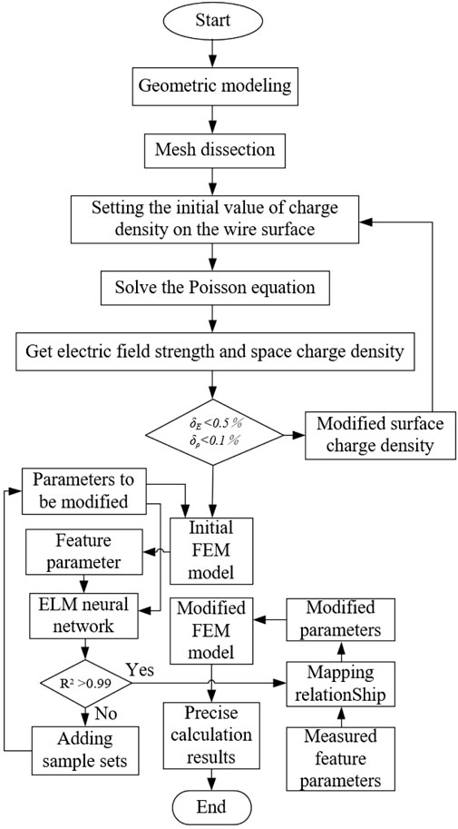
Figure 2. Flowchart.

3.2 Principles of the extreme learning machine

An extreme learning machine is an improved means of feed-forward neural network. Its most important benefit is that the weights of the hidden layer nodes are randomly given; that is, the mapping from the input layer to the hidden layer is a random mapping and does not need to be iteratively updated (Qi et al., 2024b). Compared with a BP neural network or deep learning, the ELM is more efficient and has good astringency. The neural network structure of the ELM is shown in Figure 3.

Figure 3

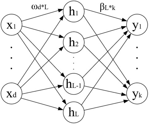
Figure 3. Structure of the extreme learning machine.

In Figure 3, x is the input layer, h is the hidden layer, and y is the output layer. The Equations 18–20 are the mathematical mechanism for the training of the extreme learning machine:

${\mathrm{h}}_{\mathrm{i}}\left(x\right)=h\left({\omega }_{\mathrm{d}*\mathrm{L}}x+b_i\right),(18)$

${\arg }_{\beta }\min ‖Y-H\left(x\right)\beta ‖2,(19)$

$f_L\left(x\right)={\displaystyle \sum _{i=1}^L}{\beta }_{i}h\left({\omega }_i,b_i,x\right),(20)$

where ω_d×L is the connection weights of the input layer x and the hidden layer h; Y is the ground truth; H(x) is the dataset matrix of the hidden layer; and β is the connection weight matrix of the hidden layer and the output layer. When the neural network is initialized, ω_d×L is randomly generated and kept constant; ω_d×L and x₁∼x_d can be nonlinearly mapped to the layer h after a composite function operation. Subsequently, the connection weights β_L×k between the output and hidden layers are computed by the least squares method.

The selection of the sample set is shown in Table 1, and the training set and validation set are assigned in a ratio of 4:1. For mesh generation, we divide the field into a near-line area A and an other area B. The three most sensitive mesh-design parameters are selected as parameters to be modified in each of these two areas (six in total). The feature parameters are selected as the ion current density ρ_j at different locations below the transmission line. Taking the center position of the tower as the reference, noted as d = 0, and extending toward the direction of the positive polarity conductor, a sample point is taken every 7.5 m, noted as d + 7.5, and vice versa. A total of nine feature parameters are selected.

Table 1

Table 1. Main parameters.

3.3 Test and modification

Taking the Jinping–Sunan transmission line (referred to as the Jinsu Line) in Huzhou, China, as an example, the electrical parameters of the Jinsu Line are shown in Table 2. The mobility of positive ions is taken as 1.5×10⁻⁴m²/(Vs.), the mobility of negative ions is taken as 1.7×10⁻⁴m²/(Vs.), and the complexity coefficient of ions is taken as 2×10⁻¹² m²/s. We measured the line, and the spatial layout obtained is shown in Figure 4A.

Table 2

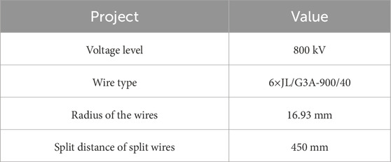
Table 2. Parameters of the Jinsu Line.

Figure 4

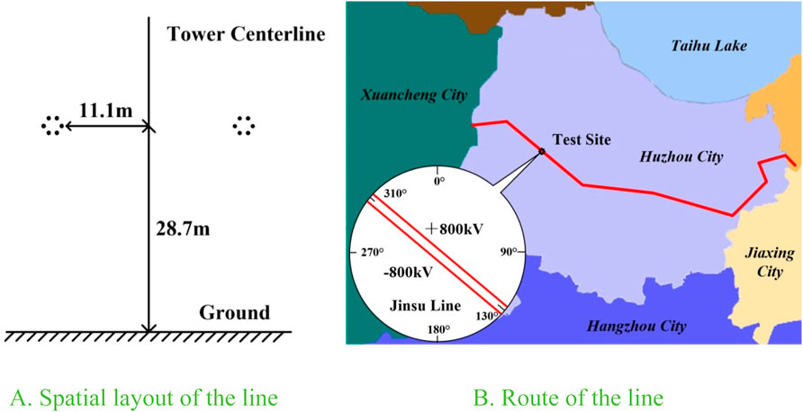
Figure 4. Geographic parameters of the line. (A) Spatial layout of the line and (B) route of the line.

Due to the introduction of wind shear, for the sake of uniformity, the following “wind speed” refers to the wind speed at the reference height (10 m); and the “wind direction” is based on the actual orientation, noting that the north wind is 0° wind direction, and the clockwise direction is positive.

Our test is located at the junction of Changxing County and Anji County, and the route of the line is shown in Figure 4B. The Jinsu Line extends from 130° southeast to 310° northwest, crossing farmland, roads, and other facilities. The wind speed on the test day was 1.92 m/s, and the wind direction was measured to be 103° toward 283°. In accordance with the requirements for the feature parameters in Section 3.2, the ion current density was measured every ±7.5 m past the center position of the line, as shown in Figure 5A, and the test photo is showed as Figure 5B.

Figure 5

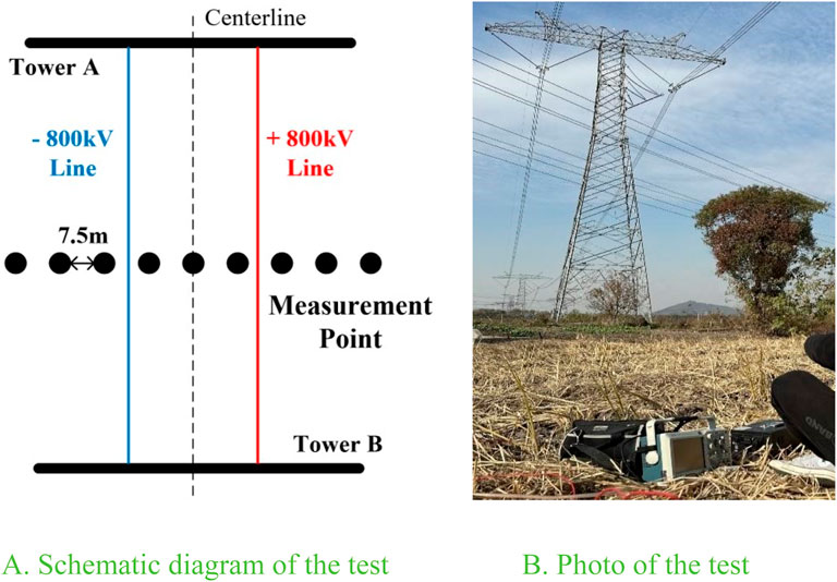
Figure 5. Test of ion current density. (A) Schematic diagram of the test and (B) photograph of the test.

In order to perform ion flow density and synthetic field measurements at the same point, a special Wilson ion flow collection plate was fabricated and machined, as shown schematically in Figure 6.

Figure 6

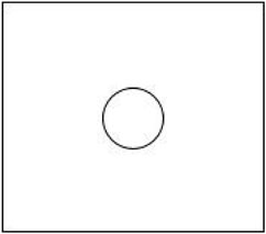
Figure 6. Schematic diagram of the Wilson collection plate.

The plate is a square copper-clad plate of dimensions 0.5 m × 0.5 m, with a circular piece in the center dug out to coincide with the area of the field strength meter for placing the electric field probe for measuring the synthetic field. The circular area is approximately 0.0056 m², so the effective area of the Wilson plate is approximately 0.2444 m². During measurement, the center of the Wilson plate coincides with the center of the electric field probe, and the upper surface of the electric field probe is flush with the Wilson plate so that the average value of the ion flow density in a certain area around the electric field strength probe represents the ion flow density in the area where the electric field strength probe is located. The placement of the measuring instrument is shown in Figure 7.

Figure 7

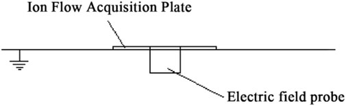
Figure 7. Placement of the measuring instrument.

The measured ion current density at the sampling point is compared with the simulation of the initial monitoring model, as shown in Figure 8. The inaccuracy of the mesh-design parameters leads to a certain deviation between the simulation and the measured results, with an average relative error of approximately 34.13%, so model modification is required.

Figure 8

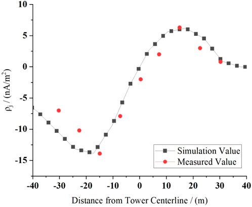
Figure 8. Comparison of the simulated and measured values.

The range of mesh parameters selection is shown in Table 3. The initial mesh parameters are randomly valued within this range to ensure the uniform distribution of sampling points. The initial monitoring model is constructed by combining the line parameters, wind speed, and direction parameters, and the values of the feature parameters are calculated. The ELM neural network was trained to obtain the coefficient of determination R² = 0.995, and a total of 1,200 sets of training samples were selected to obtain the nonlinear mapping f⁻¹.

Table 3

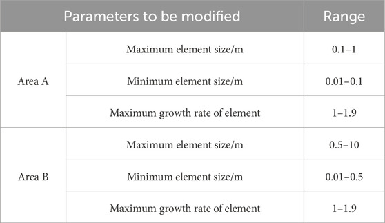
Table 3. Range of parameters.

Finally, the measured feature parameters are used as inputs to the f⁻¹ mapping to obtain the modified mesh parameters. The maximum element size is 0.47 m, the minimum element size is 0.05 m, and the maximum growth rate of the element is 1.26 for the near-line area A. The maximum element size is 6.92 m, the minimum element size is 0.18 m, and the maximum growth rate of the element is 1.43 for the other area B. The ion flow field-wind field modification model of the transmission line is constructed based on the ELM, and the mesh optimization is shown in Figure 9.

Figure 9

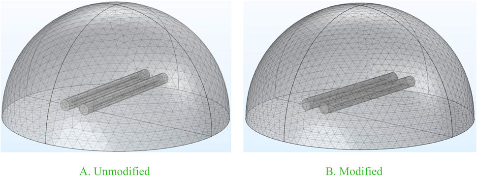
Figure 9. Mesh for finite element models. (A) Unmodified and (B) modified.

We tested again for ion current density on the second day. The wind speed on the day was 1.22 m/s, and the wind direction was 87°–267°. Figure 10 demonstrates the measured values and the calculated results of the modified model.

Figure 10

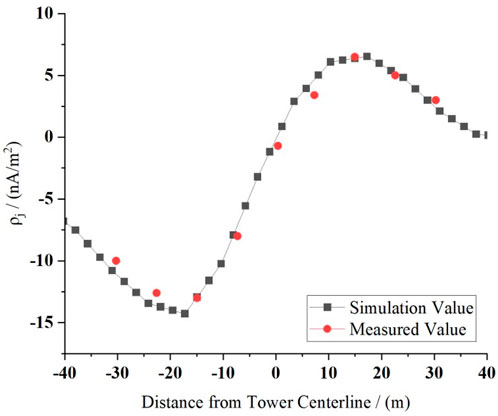
Figure 10. Comparison of the simulated and measured values after model modification.

Table 4 shows the error comparison before and after correction.

Table 4

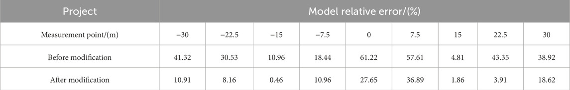
Table 4. Comparison of the relative error.

From the results, it can be seen that after the mesh modification, compared with the initial model, the simulated values fit the measured values better. The average relative error is 13.27%, and the error is reduced by 20.86%, which verifies the accuracy of the modified monitoring model. Of course, there is still a small deviation between the simulated and measured values, which is caused by the fluctuating wind.

With the same training samples, the BP neural network is used to compare with the ELM neural network to verify the superiority when corrected. The parameter settings of the BP neural network are tested to take the optimal values: the number of iterations is chosen to be 1,000, the number of neurons in the hidden layer is 3, and the learning rate is set to 0.01. A portion of the intervals of the total electric field obtained by the FEM is used as a test set to verify the neural network accuracy, as shown in the figure. The error is shown in Figure 11.

Figure 11

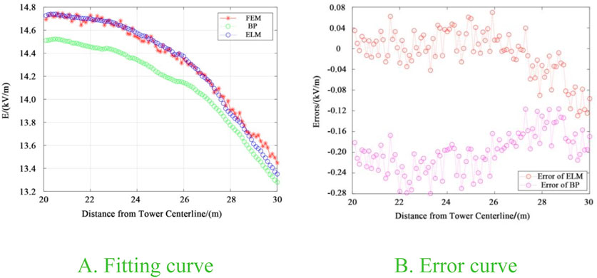
Figure 11. Comparison of ELM and BP. (A) Fitting curve and (B) error curve.

The evaluation indicators for both are shown in Table 5.

Table 5

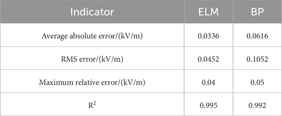
Table 5. Evaluation indicators.

Note that all the error indicators of the ELM are smaller, and the coefficient of determination is higher. The ELM model can reduce the time complexity under the premise of satisfying the fitting accuracy and has stronger applicability.

4 Calculation and analysis

4.1 Analysis of the ion flow field

The ion flow field of the Jinsu Line with wind effects is analyzed through the modified monitoring model. When there is no wind, the ions around the line are affected by the electric field force and are pushed away from the wires with their own diffusion, showing a curved moon shape as a whole and a firework shape near the wires, as shown in Figure 12. The ion distribution is concentrated in the vicinity of the wires, and the ions between two wires are recombined, with a density of 0 at the centerline position; the outer ions of the wires spread to the air domain by approximately 50 m with the density decreasing to 0. Negative ions have a stronger migratory force and diffuse more strongly than positive ions, but the overall effect is not obvious.

Figure 12

Figure 12. Distribution of the ion flow field without wind.

The ion distribution of a transverse wind (the actual direction is 220°), blowing from the − pole to the + pole of the Jinsu Line, is shown in Figure 13. The wind blows the negative ions from the upwind area (the left side of the line) to the downwind area (the right side of the line), and the ion density is almost 0 in the upwind area. In the downwind area, the positive ions are dispersed into the air domain, and the overall distribution extends outward. The greater the wind speed, the more significant is the diffusion of ions. When the wind speed is 4 m/s, most of the negative ions are blown to the vicinity of the positive polarity wire, and the positive ions are recombined, while the positive charges in the downwind area are dispersed by the extremely strong wind are nearly free from the control of the electric field force.

Figure 13

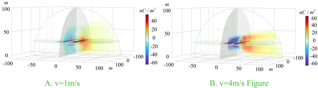
Figure 13. Distribution of the ion flow field with a transverse wind. (A) v = 1 m/s and (B) v = 4 m/s.

The distribution of ions in different wind directions is shown in Figure 14. The wind direction significantly changes the diffusion direction of the ions. The distribution is symmetrical when the wind direction and the line direction have the same angle. We can derive a law: the larger the included angle between the wind and the line, the stronger the inhibition of the wind on the diffusion of negative ions to the left; the smaller the included angle, the weaker the effect of the wind on the distribution of ions, the more obvious the diffusion of negative ions driven by the electric field force in the upwind area.

Figure 14

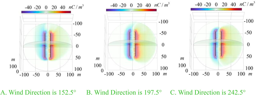
Figure 14. Distribution of the ion flow field at different wind directions. (A) Wind direction is 152.5°, (B) wind direction is 197.5°, and (C) wind direction is 242.5°.

It can be seen that the 3-D simulation results are consistent with the laws described in Equations 1–8. The migration of ions is affected by the wind, electric field force, and its own diffusion.

4.2 Analysis of ρ_j and E

Then, we analyze the absolute value of the ion current density ρ_j and the total electric field strength E. The calculation results of the modified monitoring model above demonstrate that the wind significantly affects the diffusion process of ions to the ground, making increasingly hazardous electric charges reaching the ground in the downwind area. Because negative ions have a slightly greater ability to diffuse, it is sufficient to focus on the wind blowing from the positive side to the negative side to consider the most hazardous scenario, that is, a wind direction between 310° and 130°, as shown in Figure 15, during the analysis and assessment process.

Figure 15

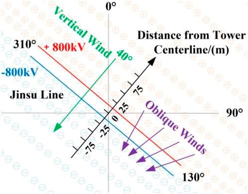
Figure 15. Wind blowing from the positive pole side to the negative pole side.

When the wind is a transverse wind, blowing from the + pole to the − pole (40° wind direction), the distribution pattern of ion current density ρ_j is shown in Figure 16. Taking the windless situation as a reference, when there is no wind, the distribution of ρ_j below the positive and negative polarity wires of the Jinsu Line is almost symmetrical, and the peak value of negative ion current density is approximately 11.30 nA/m². With the increase in the wind speed, the curve of ρ_j under the wires shifts to the downwind area: the ρ_j under the positive polarity wires decreases sharply, and decreasing amounts of positive electric charge reach the ground. This value is reduced to zero at the wind speed of 3 m/s. The absolute value of ρ_j under the negative polarity wire increases and then decreases when the wind speed is 4.4 m/s. ρ_j increases to 19.16 nA/m², an increase of approximately 69.56%, and the peak position of the curve is shifted to −31.80 m from −17.24 m in the downwind area. Then, the peak absolute value decreases gradually, and the value decreases to 13.06 nA/m² when the wind speed is 7 m/s and further decreases with increased wind speed.

Figure 16

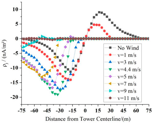
Figure 16. Transverse wind influence on ion current density.

The variation of the total electric field strength E is shown in Figure 17, where the decrease in E in the upwind area is significantly stronger than the increase in E in the downwind area. The E below the positive polarity wire is approximately 14.82 kV/m when there is no wind, and the value gradually decreases to a nominal electric field strength of 6.61 kV/m with the increase in wind speed, which is a decrease of approximately 55.40%. While the absolute value of E below the negative polarity conductor increases and then decreases with the increase in wind speed, it is raised to the maximum value of 19.74 kV/m at the wind speed of 4.4 m/s, with an increase of approximately 33.20%. The value decreases to 11.99 kV/m when the wind speed reaches 11 m/s. As for the change of the peak location, the E is not as significant as that of the ρ_j, and the area of the peak absolute value of E is concentrated in the downwind area from approximately −45 m to the −15 m position.

Figure 17

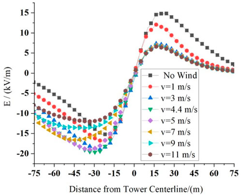
Figure 17. Transverse wind influence on total electric field strength.

When the wind direction changes, the changes in ρ_j and E occur as shown in Figures 18, 19. The effect of wind direction on ρ_j and E is mainly reflected in the included angle between the wind direction θ and the line direction. When this angle is the same, the effect on ρ_j and E is the same. When the wind direction θ is parallel to the line direction, the simulation is in an ideal situation and does not take into account the length limitation of the wires, so the ion flow will not be affected by the parallel wind to diffuse to the outer side of the wires, and, therefore, ρ_j and E are almost unaffected by the parallel wind.

Figure 18

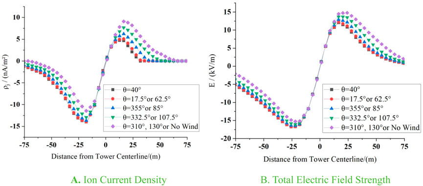
Figure 18. Trends at low wind speed. (A) Ion current density and (B) total electric field strength.

Figure 19

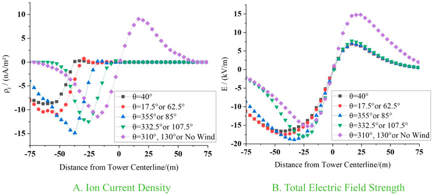
Figure 19. Trends at high wind speed. (A) Ion current density and (B) total electric field strength.

From Figure 18, it is easy to find that at low wind speed, when the wind speed is 1 m/s, the maximum absolute value of ρ_j appears at θ = 40°, and ρ_j = 14.05 nA/m² is calculated. As the included angle between the wind direction and the line direction decreases, the minimum absolute value of the peak ρ_j appears at θ = 310° or 130°, and ρ_j = 11.30 nA/m² is calculated. The change of the peak total electric field strength also satisfies a similar law. The maximum absolute value of E is calculated to be 17.01 kV/m, and the minimum absolute value of the peak E is 15.3 kV/m. It can be found that when the wind speed is low, the smaller the included angle between the wind direction θ and the line direction is, the smaller the absolute values of peak ρ_j and E are.

From Figure 19, it is easy to find that the law changes in high wind speed. When the wind speed is 8 m/s, the minimum absolute value of peak ρ_j occurs at θ = 40°, with a value of 8.67 nA/m². Then, with the decrease of the included angle between the wind direction θ and the line direction, the maximum absolute value of ρ_j occurs at θ = 355° or 85°, with a value of 15.49 nA/m², and the peak value of ρ_j is reduced to 11.3 nA/m² with the further decrease of the included angle between the wind direction θ and the line direction. The absolute value of peak E also satisfies a similar law. The minimum absolute value of peak E is calculated to be 15.31 kV/m, and the maximum absolute value is calculated to be 18.93 kV/m. It can be found that, at high wind speed, the absolute values of peak ρ_j and E increase and then decrease as the included angle between the wind direction and the line direction decreases.

Therefore, when constructing HVDC transmission lines, the wind speed and direction distribution in each region should be considered to minimize the impact of wind, thus reducing the hazards of the ion flow field and total electric field of the HVDC transmission line.

5 Conclusion

As the demand for electricity in the power system increases, a balance must be struck between energy delivery efficiency and environmental compatibility, and condition monitoring and analysis have become major issues in ensuring the safety and reliability of the power system during transmission and distribution. The ion flow field formed by the (UHVDC) transmission line is migrated by the wind, which intensifies the ground ion current density ρ_j and the total electric field strength E and produces serious electromagnetic hazards. Aiming at the problem that ρ_j and E are difficult to monitor, this article takes the ±800 kV Jinsu Line in Huzhou as an example and constructs a monitoring model of the ion flow field of the transmission line considering different speeds and directions of winds. The model is modified by the ELM neural network to realize the accurate monitoring and characterization study and obtain the following conclusions.

(1) The monitoring model is modified so that the relative error between the simulated and measured values is 13.27%, and the accuracy is improved by 20.86%. The monitoring model can make accurate calculations at different wind speeds and directions.

(2) When the wind is transverse, the ion current density and total electric field strength increase and then decrease with the wind speed. The peak case occurs at 4.4 m/s.

(3) When the wind direction changes at low wind speeds, the smaller the included angle between the wind direction and the line direction, the smaller the absolute value of peak ρ_j and E. At high wind speeds, as the included angle is smaller, the absolute values of peak ρ_j and E first increase and then decrease.

Data availability statement

The original contributions presented in the study are included in the article/supplementary material, further inquiries can be directed to the corresponding author.

Author contributions

ZQ: Conceptualization, Data curation, Formal Analysis, Investigation, Methodology, Project administration, Resources, Software, Supervision, Validation, Visualization, Writing – original draft, Writing – review and editing. JC: Conceptualization, Data curation, Formal Analysis, Funding acquisition, Investigation, Methodology, Resources, Software, Supervision, Validation, Writing – original draft, Writing – review and editing. MR: Conceptualization, Data curation, Funding acquisition, Investigation, Resources, Software, Supervision, Validation, Visualization, Writing – original draft, Writing – review and editing. FY: Conceptualization, Data curation, Formal Analysis, Investigation, Methodology, Software, Supervision, Validation, Visualization, Writing – original draft, Writing – review and editing.

Funding

The author(s) declare that no financial support was received for the research and/or publication of this article.

Conflict of interest

Authors MR and FY were employed by East China Branch, State Grid Corporation of China.

The remaining authors declare that the research was conducted in the absence of any commercial or financial relationships that could be construed as a potential conflict of interest.

Generative AI statement

The author(s) declare that no Generative AI was used in the creation of this manuscript.

Publisher’s note

All claims expressed in this article are solely those of the authors and do not necessarily represent those of their affiliated organizations, or those of the publisher, the editors and the reviewers. Any product that may be evaluated in this article, or claim that may be made by its manufacturer, is not guaranteed or endorsed by the publisher.

References

Bai, X., Wang, Y., Cui, R., Wu, M., Chen, Y., and Lv, J. (2023). Selection of polarity distance for ±800kV DC transmission lines at ultra high altitude. 51(04):52–56. doi:10.16109/j.cnki.jldl.2023.04.012

Cai, H., Du, Z., Xiu, L., Yue, G., He, J., and Li, E. (2023). Calculation and measurement of ion flow field of UHVDC transmission line at high altitude and high wind speed. Adv. Technol. Electr. Eng. Energy 42 (08), 32–40. doi:10.12067/ATEEE2207050

Chen, W. (2014). Discussion on electromagnetic environment monitoring of high voltage DC transmission Project. Technol. Innovation Appl. 2014 (21), 34–36. doi:10.19981/j.cn23-1581/g3.2014.21.025

Choopum, C., and Techaumnat, B. (2022). Numerical investigation on the effects of wind and shielding conductor on the ion flow fields of HVDC transmission lines. Energies 16 (1), 198. doi:10.3390/en16010198

Cui, X., Zhou, X., and Lu, T. (2012). Recent progress in the calculation methods of ion flow field of HVDC transmission lines. Proc. CSEE 32 (36), 130–141+3. doi:10.13334/j.0258-8013.pcsee.2012.36.020

Di, H., Yan, Y., Zhao, M., and Kang, M. (2022). Design and validation of reversing assistant based on extreme learning machine. Front. Energy Res. 10, 914026. doi:10.3389/fenrg.2022.914026

Du, Z., Xiu, L., He, J., and Cai, H. (2022). Computation of total electric field considering natural wind under high-altitude UHVDC transmission lines. IEEE Trans. Magnetics 58 (09), 1–4. doi:10.1109/TMAG.2022.3186483

Huang, G., Zhou, H., Ding, X., and Zhang, R. (2012). Extreme learning machine for regression and multiclass classification. IEEE Trans. Syst. 42, 513–529. doi:10.1109/TSMCB.2011.2168604

PubMed Abstract | CrossRef Full Text | Google Scholar

Huang, G. B., Zhu, Q. Y., and Siew, C. K. (2006). Extreme learning machine: theory and applications. Neurocomputing 70, 489–501. doi:10.1016/j.neucom.2005.12.126

Janischewskyj, W., and Cela, G. (1979). Finite element solution for electric fields of coronating DC transmission lines. IEEE Trans. Power Apparatus Syst. PAS-98 (3), 1000–1012. doi:10.1109/TPAS.1979.319258

Kang, Y., Pu, X., Zhang, J., Zhao, S., Chen, Z., Ma, Z., et al. (2024). Characterization of ion flow in ±800 kV HVDC transmission line under bidirectional coupling of flow field and ion flow field. Proc. CSEE 44 (22), 9087–9099. doi:10.13334/j.0258-8013.pcsee.231573

Li, Y., Zou, A., Xu, L., and Zhang, H. (2012). Calculation on corona ionized field of UHVDC transmission lines by finite element-integral method. High. Volt. Eng. 38 (06), 1428–1435. doi:10.3969/i.issn.1003-6520.2012.06.021

Lin, Y. (2024). Study on corona discharge characteristics of UHV transmission line ground wire surface under thundercloud electric field. Shandong Univ. Technol. 2024 (05). doi:10.27276/d.cnki.gsdgc.2023.000845

Lu, C., Xiao, D., and Qin, S. (2014). Calculation of hybrid electric field under the parallel AC/DC transmission lines and its experimental research. High. Volt. Appar. 50 (01), 81–86+91. doi:10.13296/j.1001-1609.hva.2014.01.015

Lu, T., Feng, H., and Cui, X. (2008). Research on total electric field beneath HVDC power lines based on upstream finite element method. Power Syst. Technol. 2008 (02), 13–16+25. doi:10.3724/SP.J.1001.2008.01274

Lu, T., Feng, H., Cui, X., Zhao, Z., and Li, L. (2010). Analysis of the ionized field under HVDC transmission lines in the presence of wind based on upstream finite element method. IEEE Trans. Magnetics 46 (8), 2939–2942. doi:10.1109/TMAG.2010.2044149

Lu, T., Feng, H., Zhao, Z., and Cui, X. (2007). Analysis of the electric field and ion current density under ultra high-voltage direct-current transmission lines based on finite element method. IEEE Trans. Magnetics 43 (4), 1221–1224. doi:10.1109/tmag.2006.890960

Park, Y., Jha, R., Park, C., Rhee, S. B., Lee, J., and Park, C. G. (2018). Fully coupled finite element analysis for ion flow field under HVDC transmission lines employing field enhancement factor. IEEE Trans. Power Deliv. 33 (6), 2856–2863. doi:10.1109/TPWRD.2018.2854678

Qi, L., Kawaguchi, T., and Hashimoto, S. (2024a). A series arc fault diagnosis method based on an extreme learning machine model. Processes 12 (12), 2947. doi:10.3390/PR12122947

Qi, W., Hao, S., Zhou, Y., and Xun, D. (2024b). Research on improving electromagnetic environment of mixed-voltage double circuit DC transmission line on the same tower. Environ. Technol. 42 (03), 183–190. doi:10.3969/j.issn.1004-7204.2024.03.037

Qiao, J., Ge, X., and Zou, J. (2019). A flux tracing-finite element hybrid method for calculating ion-flow field of HVDC overhead lines in presence of wind. Trans. China Electrotech. Soc. 34 (05), 910–916. doi:10.19595/j.cnki.1000-6753.tces.180144

Tadasu, T., Tsutomu, I., and Tadashi, K. (1981). Calculation of ION flow fields of HVDC transmission lines by the finite element method. IEEE Trans. Power Apparatus Syst. PAS- 100 (12), 4802–4810. doi:10.1109/TPAS.1981.316432

Wan, Y. (2023). Study on conductor type selection of ±800kV UHVDC lines in xinjiang. (23), 91–93. doi:10.19768/j.cnki.dgjs.2023.23.025

Wang, W., and Chen, W. (2015). Monitoring and analysis of electromagnetic environmental impacts of high-voltage direct current transmission lines. J. Hefei Normal Univ. 33 (06), 17–18+23. doi:10.3969/j.issn.1674-2273.2015.06.005

Wen, C., Yan, Z., and Wu, X. (1985). Measurements and analysis of corona onset voltage of HVDC test line and ion current density at ground level. High. Volt. Eng. 1985 (03), 24–28. doi:10.13336/j.1003-6520.hve.1985.03.006

Wu, H. (2019). Study on electromagnetic environment of EHV/UHV AC-DC parallel transmission lines. Chongqing Univ. 2021 (01). doi:10.27670/d.cnki.gcqdu.2019.000788

Xu, J., Wan, B., and Xie, H. (2020). Analysis of measurement on total electric field of a ±800kV DC transmission line with wind’s speed less than 2 m/s. IET Conf. Proc. 2020 (01), 310–316. doi:10.1049/icp.2020.0082

Xu, Y., Liang, Z., and Zhang, Y. (2023). Research on induced electrical characteristics of double circuit hybrid voltage DC transmission lines on the same tower. 48(4), 913–920. doi:10.13624/j.cnki.issn.1001-7445.2023.0913

Yang, X., Lv, J., Tang, L., Peng, J., and Huang, T. (2015). Calculation and test of resultant electric field at the ground level under UHVDC parallel double-circuit transmission line. High. Volt. Appar. 51 (07), 46–51. doi:10.13296/j.1001-1609.hva.2015.07.009

Yi, Y., Wang, L., and Chen, Z. (2022). Estimating the environmental impacts of HVDC and UHVDC lines for large-scale wind power transmission considering height-dependent wind and atmospheric stability. Int. J. Electr. Power and Energy Syst. 2022 (138), 107868–107910. doi:10.1016/j.ijepes.2021.107868

Zhang, J., Zhang, G., Zhang, X., Wan, B., Wu, X., and He, J. (2009). Simulation experiment and calculation of DC electric field caused by DC transmission line at high altitude districts. High. Volt. Eng. 35 (08), 1970–1974. doi:10.13336/j.1003-6520.hve.2009.08.030

Zhang, W., Yu, Y., Li, G., Fan, J., Su, Z., Lu, J., et al. (2007). Researches on UHVDC technology. Proc. CSEE 27 (22), 1–7. doi:10.3321/j.issn:0258-8013.2007.22.001

Zou, A., Wang, S., Yang, T., Li, Y., and Liu, Y. (2023). Calculation of synthetic electric field of UHVDC transmission line based on BPA method. Water Resour. Power 41 (05), 194–198. doi:10.20040/j.cnki.1000-7709.2023.20221431

Zou, A., Xu, L., Ji, Y., Gong, L., Hou, X., and Wu, G. (2017). Review of the researches on finite element calculation of ion flow field for DC transmission lines. High. Volt. Appar. 53 (11), 27–33. doi:10.13296/j.1001-1609.hva.2017.11.005

Zou, J., Cheng, Q., Qiao, J., Zhang, Y., and Jiang, L. (2020). Review on ion current field calculation in HVDC power transmission line. South. Power Syst. Technol. 14 (06), 1–10. doi:10.13648/j.cnki.issn1674-0629.2020.06.001