Prediction of electricity production by small wind power using artificial neural networks

Introduction: Wind energy is one of the most significant and rapidly growing renewable energy sources worldwide. It is a clean and environmentally friendly form of energy production, which emits no harmful substances or greenhouse gases during the power generation process. There has been a growing interest in research in the field of wind energy. In this article, an artificial neural network method is used to evaluate the forecasting of wind energy production from a small wind turbine (SWT) installed in central Poland, reflecting inland wind conditions.

Methods: A comprehensive set of algorithms and results from simulations are presented. An artificial neural network (ANN) is trained and verified using a large observation dataset. The model includes four input variables: wind speed and direction, rotor speed, air temperature, and one output variable - the power generated by the turbine. Among the available neural networks, Multilayer Perceptron was selected. Genetic algorithms were used to optimize the structure of the model. The Pearson correlation coefficient was used to assess the correspondence between the predicted values and the actual ones. The modeling was carried out in MATLAB, and coefficients such as Mean Squared Error (MSE), Root Mean Squared Error (RMSE), and Mean Absolute Percentage Error (MAPE) were used to evaluate the prediction error.

Results and Discussion: The learning and testing performance of the neural network model using back propagation with feedback was 96.3% and 97.0%, respectively. Additionally, a sensitivity analysis of the predictive model was performed. The neural network model presented in the article provides accurate predictions of the power generated by a wind turbine. The results obtained confirm the effectiveness of the use of MLP-type neural networks in tasks related to the prediction of energy production in small wind turbines in inland locations.

1 Introduction

With growing energy demand driven by economic development and improved living standards, reliance on fossil fuels poses serious environmental challenges, including pollution and global warming (Gómez and García, 2018; Wang et al., 2019). Given their limited and non-renewable nature, fossil fuel overuse accelerates resource depletion. In this context, renewable energy, particularly wind power, emerges as a key alternative. Widely adopted worldwide, wind energy plays an increasingly important role in smart grids, buildings, and homes (Wang et al., 2021).

According to the Directive on the Promotion of the Use of Renewable Energy, by 2030, the share of renewable energy sources (RES) in the gross final energy consumption in the European Union (EU) is expected to reach 42.5%. Another ambitious goal for the EU is to achieve climate neutrality by 2050. Currently, all EU member states have targets for the share of renewable energy in the national energy mix, which they must meet by 2030 (European sources, 2023; Consilium, 2023). Therefore, there is an acceleration of the transition to clean energy by increasing the share of RES in power generation, industry, construction, and transportation.

Wind energy is one of the fastest growing renewable energy sources and is widely regarded as an interesting alternative to conventional fossil fuel energy sources. In 2022, 77.6 GW of new wind capacity was connected to electricity grids worldwide, bringing the total installed wind capacity to 906 GW (9% increase compared to 2021). Thus, 2022 was the third best year ever in terms of new capacity (Global Wind Energy Council, 2023).

The wind power market is growing rapidly, so there is a strong need for development in this field for both technical and economic progress. This motivates researchers to conduct analysis and prediction of wind power generation. When considering technical aspects, maximizing the yield of wind potential is taken as the goal. On the other hand, with regard to economic issues, intentionality is turned to obtaining maximum profits from the available resources (Marugán et al., 2018). While technically aimed at maximizing energy yield, forecasts also help secure financial returns. Due to the variability of wind, reliable prediction remains a complex challenge—yet it is essential for energy trading, grid stability, and reducing economic risks, especially for small wind turbine owners. Forecasts are crucial for wind farm owners and operators, distribution and transmission system operators, and maintenance teams.

Accurate wind power forecasts improve power system efficiency by helping align generation with demand, optimize energy storage, and support bidding strategies in electricity markets (Kim and Powell, 2011; Zugno and Conejo, 2015; Gómez et al., 2017). They also aid in real-time turbine control, maintenance planning, and grid management, enabling operators to balance loads and ensure system stability (Okumus and Dinler, 2016). Thus, predictive models are vital for sustainable and efficient energy system operation.

The rapid growth of wind energy has increased the need for accurate forecasting tools. Effective predictions should consider key parameters and reflect future trends. Forecasts support balancing supply and demand, grid optimization, and planning reserves (Hossa et al., 2014; Sweeney et al., 2020). However, due to the variability of atmospheric conditions, wind energy is difficult to predict reliably, and minimizing forecast errors remains a major challenge (Augustyn and Kamiński, 2018; Mentes et al., 2012).

Wind is highly variable in time and space, influenced by meteorological and geographical factors. This variability, along with uncertainties in weather forecasts and turbine conditions, poses major challenges for predicting wind power generation (Kou et al., 2013; Markowicz, 2011; Özgür, 2014). In terms of evaluating forecasts made for wind power, it is also important to use different ways of developing forecasting methods, leading to different criteria for evaluating methods and their results (Popławski et al., 2013).

Wind power forecasting methods can be divided into physical and statistical depending on the modeling approach. Physical forecasting methods are based on converting data resulting from the numerical weather prediction system (NWP) into wind turbine data. They then forecast wind power based on the predicted wind speed and turbine power curve. Statistical methods are based on the analysis of a large amount of historical data and use various statistical models to predict wind power, such as time series analysis and machine learning algorithms (Li et al., 2023). Furthermore, some solutions based on statistical models are introduced as a hybrid algorithm in combination with NWP models (Pourmousavi Kani and Ardehali, 2011).

The development of computer technology has contributed to the popularization of predictive models based on artificial intelligence, among which artificial neural networks (ANN) (Ak et al., 2018; Liu Y. et al., 2020), support vector machines (SVM) (Liu M. et al., 2020), fuzzy logic (Severiano et al., 2021), through which it is possible to capture the features of nonlinearity contained in the input data (Heng et al., 2022). Neural networks are the most widely used tool in artificial intelligence methods for forecasting electricity production (Drałus and Gomółka, 2017; Jiménez et al., 2018). The main advantages of the ANN approach are the model’s ability to self-learn, self-organize and self-improve.

In recent years, researchers around the world have been conducting numerous studies to predict wind power output. Many reviews of wind power prediction have been published with various approaches (Foley et al., 2012; Marugán et al., 2018). Wang et al. (2021) reviewed the literature on various DNN (Deep Neural Networks) models and analyzed their effectiveness in predicting wind speed and wind power. The publication (Wang K. et al., 2018) applied the k-means clustering algorithm to process numerical weather prediction (NWP) data and, in turn used a deep belief network (DBN) for short-term wind power forecasting.

Xiao et al. (2021) proposed an effective high-performance learning model, the kernel extreme learning machine (KLEM). Han et al. (2022) presented a new short-term wind speed prediction method using advanced hybrid deep learning algorithms to improve numerical weather forecasting (WRF). The paper (Liu H. et al., 2020) develops a new hybrid ensemble deep reinforcement learning model for short-term wind speed forecasting.

The paper (Wang et al., 2020) discusses a hybrid Laguerre neural network model for wind energy prediction with multi-stage advance. Yan et al. (2019) trained a geometric model artificial neural network (GM-ANN) based on offshore wind farm observation data. They proposed a two-dimensional (2-D) power curve that allowed one to estimate the generated power by a wind farm based on wind speed and direction. Sun et al. (2020) proposed a power prediction model and optimized the deviation angles to minimize the total impact of the track footprint on wind turbines. Zameer et al. (2017), for short-term wind energy prediction, proposed a model based on ANN genetic programming. Nielson et al. (2020) used ANN to generate multi-parameter input models to estimate the power generated by a wind turbine. In his work, Blonbou (2011) used the wind speed and power from the previous time step to train the SSN using adaptive Bayesian learning and Gaussian process approximation. In the publication (Qureshi et al., 2023) the authors examine the application of various artificial intelligence techniques for forecasting wind power generation and analyze their effectiveness and precision. The paper (Taghinezhad and Sheidaei, 2022) discusses an advanced ANN adapted to diffuser wind turbine systems.

The scientific literature is dominated by topics related to large wind turbines, due to their widespread use in utility power systems and a wealth of operational data. In contrast, small wind turbines (SWTs), which are playing an increasingly important role in local, decentralized power systems (e.g., for domestic, agricultural or off-grid purposes), are much less frequently analyzed. The current state of research on forecasting SWT-generated power is limited, especially in the context of applying artificial intelligence methods such as artificial neural networks. Most of the available work focuses on large installations, which creates an important research gap in the area of small units. This work aims to partially fill this gap by proposing an ANN-based predictive model for a specific small wind turbine.

By SWT, we mean a wind turbine with a power rating of less than 50 kW and a rotor area of less than 200 m² (Zalewska et al., 2021). These turbines are more affordable and have lower operating and maintenance costs, making them a reliable solution for off-grid rural and suburban areas. Among other things, small wind turbines can generate decentralized energy and reduce energy bills for consumers and power purchase costs for distribution companies, as well as help manage periods of peak demand (Zishan Akhter et al., 2023; Eltayesh et al., 2023). It is concluded that they represent an economically viable and beneficial solution in the area of renewable energy that can contribute to the achievement of the Sustainable Development Goal (SDG 7) of providing affordable access to clean energy for all. These goals were included in the 2030 Agenda for Sustainable Development, which was adopted by all the UN member states in 2015 (IEA et al., 2022). However, the commercial success of these turbines depends on the economic feasibility of the energy produced, which is determined by the initial cost per unit of power and the unit cost per kilowatt hour (kWh) produced (Tummala et al., 2016). Therefore, it is worth focusing on the prediction of energy from small wind turbines, which is done in this paper.

The paper demonstrates the potential of artificial neural networks (ANNs) to predict the generated power of a small wind turbine. The network is trained and verified using a large dataset of observations of air temperature, wind speed and direction, and turbine rotor speed. The prediction of energy from small wind turbines (SWTs). The novelty aspects of the paper are based on the new methodology developed for the study based on the proposed neural network and the experimental data incorporated for this study. It should be emphasized that the developed model can be useful for energy planners and wind turbine owners who are looking for the effectiveness of neural networks for the energy production of SWTs.

The article is structured as follows: Chapter 1 is an introduction, which includes the basics of turbine power prediction and a review of the literature in the area under study. Chapter 2 presents the methodology developed for the study, the theoretical assumptions of the model, the input parameters, and the structure of the proposed neural network. This chapter also presents a case study of the analyzed wind turbine and describes the data collection. Chapter 3 presents the wind power forecasting model and the results from the study, as well as the sensitivity analysis of the results. The conclusions of the article and the conclusions are included in Chapter 4.

2 Materials and methods

2.1 Wind turbine power prediction model

2.1.1 Artificial neural network

Machine learning algorithms are widely used due to their ability to process large amounts of data, and one of the most widely used methods is ANN (Jóźwiak and Lesiak, 2020). Artificial neural networks can learn from data and use this knowledge, leading to their widespread use in various fields, such as an advanced tool for modeling, classification, identification, prediction, and control (Karaman, 2023). Learning a neural network involves searching the parameter space of the network for an optimal set of weights that provide a good fit of the target input-output relationship. Artificial neural networks are trained by historical data sets to understand the relationship between output and input variables.

The ANN model consists of various layers, including an input layer, one or more hidden layers, and an output layer. The input layer is responsible for receiving input data, which is then processed by hidden layers, ultimately leading to the generation of the final output by the output layer. The hidden layers play a key role in transforming the input data through a set of weighted connections and activation functions, enabling the network to understand complex patterns and relationships in the data. Each layer contains numerous neurons that connect to each other through connections between successive layers of multilayer networks; neurons are connected between layers on a peer-to-peer basis (typically, neurons of nearby layers are connected). This allows modeling the nonlinear dependence of the output variable on the input variable (Babbar and Langah, 2022; Augustyn and Kamiński, 2018).

The first step in building an ANN model is to choose a neural network topology. These include unidirectional networks, in which information flows in one direction, recurrent neural networks, where neurons send feedback signals to each other, and competitive learning networks (Senthil Kumar, 2019). The next step is to choose the appropriate learning algorithm. Learning can be supervised - the network’s task is to learn a function that determines the dependence of the output variable on the input variables based on a historical data set consisting of input-output pairs. The second option is unsupervised learning, which involves determining the parameters of the ANN depending on the dataset and the cost function. The third type is reinforcement learning, in which input data is generated by interacting with the environment (Rahman et al., 2021; Jung and Broadwater, 2014). The performance of artificial neural networks depends on many different factors, including data preprocessing, data structure, learning method, connections between input and output data (Marugán et al., 2018).

In this article, the authors chose to use artificial neural networks due to their high efficiency and precision in wind energy forecasting. This was confirmed and presented in the article (Jamii et al., 2022). Jamii et al. compared the performance of the ANN model with four other machine learning-based techniques (LASSO, decision tree, regression vector machines, and kernel ridge regression). The results showed that all techniques could learn quickly and provide accurate power predictions. However, the ANN model provided the best forecasting accuracy, outperforming other methods. In addition, ANN proved to be a useful tool for optimal power planning and management. Therefore, it was decided to choose the ANN model. There are many types of ANN models for a given problem depending on various parameters such as function complexity, architecture, training algorithm, and number of training cases (Varshney and Poddar, 2012). In this article, multilayer perceptron (MLP) was chosen, which is considered the most popular type of artificial neural networks.

2.1.2 Multilayer perceptron

MLP is an artificial feedforward neural network (FNN) used in regression (Ziółkowski et al., 2021) and classification (Zanaty, 2012). MLP is built with three types of neuron layers: input, hidden, and output. The input neurons represent the values of the independent variables, and their number is determined by the number and type of input parameters. The hidden layers are responsible for processing the signals, while the output neurons represent the predicted values of predictor variables. Figure 1 shows the general architecture of the MLP, consisting of four input neurons, one output neuron and an unspecified number of hidden neurons arranged in four layers. The number of neurons in each hidden layer and the activation functions of each layer are subject to optimization using a genetic algorithm.

Figure 1

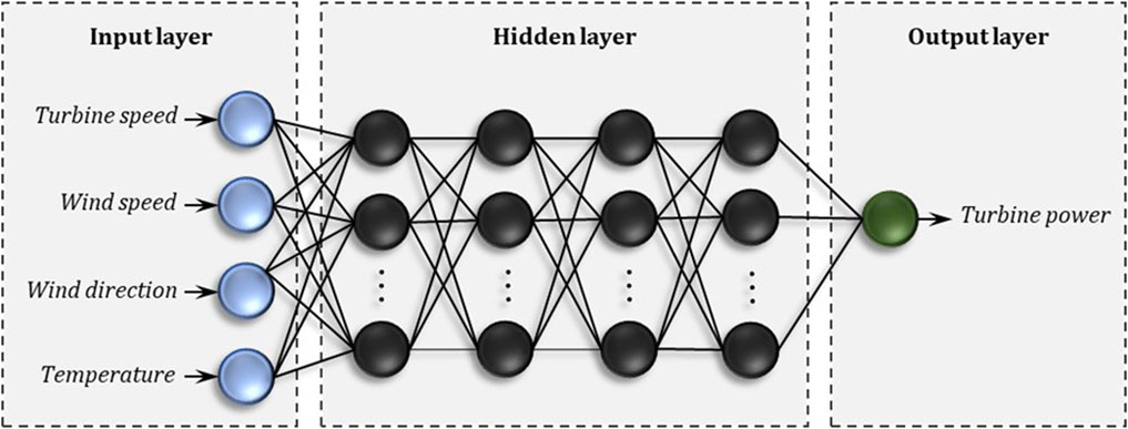
Figure 1. Multi-layer feed-forward neural network architecture.

The input signals are normalized values of the independent variables (turbine speed, wind speed, wind angle sine, air temperature). Normalization brings the values of the variables into the interval [0, 1] (Al-Ghamdi et al., 2021; Henderi, 2021; Chia et al., 2022), according to Formula 1:

$x_{norm}=\frac{x_{\mathit{max}}-x}{x-x_{\mathit{min}}}.(1)$

The regression problem involves predicting the value of turbine power, which is assumed to be a non-negative value. For this reason, normalization of the value of the predicted variable, based on the natural logarithm, was used (Al-Naser et al., 2016), according to Formula 2:

$y_{norm}=\ln \left(y\right).(2)$

On the other hand, Formula 3 is used to calculate the projected value $y_{pred}$ of the turbine power based on the output value:

$y_{pred}=e^{y_{norm}}.(3)$

This approach avoids negative values in the output of the network. In fact, the MLP predicts the value of the power exponent for a base equal to e, and then the inverse normalization determines the value of the turbine power prediction. The mathematical properties based on Formula 4 show that:

${\forall }_{y_{norm}\mathfrak{\in }\mathfrak{R}}{e}^{y_{norm}}>0.(4)$

Five types of aggregated signal activation functions were considered entering the neurons in the hidden and output layers (Bircanoglu and Arica, 2018; Garud et al., 2021):

— Linear

$f\left(x\right)=x,(5)$

— Sigmoid

$f\left(x\right)=\frac{1}{1+e^{-x}},(6)$

— Hiperbolic tangent (tanh)

$f\left(x\right)=\tanh x=\frac{e^x-e^{-x}}{e^x+e^{-x}},(7)$

— ReLU

$f\left(x\right)=\mathit{max}\left(0,x\right)=\left\{\begin{array}{l}xifx>0\\ 0otherwise\end{array}\right.(8)$

— Softmax

$f\left(x_i\right)=\frac{e^{x_i}}{{\displaystyle {\sum }_{j=1}^n}{e}^{x_j}}(9)$

2.1.3 Genetic algorithm

Genetic algorithms (GAs) are a subclass of stochastic evolutionary algorithms of global search for the extreme values of the objective function. GA is a mathematical model of the Darwinian process of gene evolution (Tajmiri et al., 2020). In the optimization of the neural network architecture, a chromosome is defined as a set of genes that represent hyperparameters not subject to the learning process. In the proposed approach, the chromosome encoding the neural network is made up of nine genes. The first four genes determine the number of neurons in the following hidden layers. The next four genes provide information about the activation function of the corresponding hidden layers, and the last, ninth, gene is responsible for the activation function of the output layer. The number of neurons is a positive integer from the accepted range, while the activation functions are selected from a set of permissible functions, determined by Formulas 5–9. A schematic of the MLP-encoding chromosome is shown in Figure 2.

Figure 2

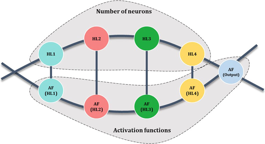
Figure 2. Chromosome of artificial neural network.

The first step in optimizing the MLP architecture is the collection and pre-processing of a suitable database of wind turbine efficiency. Based on the normalized empirical data, the process of learning, validation, and testing of neural networks is carried out. For this reason, a division of the data set into three subsets was adopted in standard 60/20/20 proportions.

The genetic algorithm requires the definition of its basic parameters and methods. For genes encoding the number of hidden neurons, intermediate recombination was adopted as the crossover method. If two neural networks as parents of the future generation have the number of neurons ${\mathrm{\alpha }}_{\mathrm{i}}$ and ${\mathrm{\beta }}_{\mathrm{i}}$ for the hidden layer i respectively, their crossover will result in networks having the number of neurons in the hidden layer and equal to ${\mathrm{\gamma }}_{\mathrm{i}}$, according to the Formula 10 (Wang Y. et al., 2018):

${\gamma }_i={\alpha }_i·p+{\beta }_i·\left(1-p\right),(10)$

where p is a random number from a uniform distribution defined on the interval [−d, 1+d], with d being some assumed constant value.

The crossing of genes encoding activation functions is carried out according to the uniform crossover method (Yi et al., 2020; Kurdi, 2019). The probability from selecting a gene of a given parent is equal to 0.5.

The process of mutation aims to solve the problem of trapping the local extremes that the target function reaches. Through mutation, a greater diversity of chromosomes is achieved in the population. Genes encoding the number of neurons and genes encoding activation functions can undergo the mutation process with a certain probability p; however, the mutation process itself in both cases is different (Garud et al., 2021; Luo et al., 2020). For the number of neurons, because it is expressed as a positive integer in a certain range, the mutation follows a normal distribution and according to the law of three sigma. If crossover results in a gene ${\mathrm{\gamma }}_{\mathrm{i}}$, then after mutation it is expressed as ${\mathrm{\gamma }}_{\mathrm{i}}^{\prime }$, according to the relation (Formula 11):

${\gamma }_i^{\prime }={\mathrm{\gamma }}_{\mathrm{i}}+\mathcal{N}\left(0,\sigma \right),(11)$

where $\sigma$ is equal:

$\sigma =\frac{{\mathrm{\gamma }}_{\max }-{\mathrm{\gamma }}_{\min }}{6}.(12)$

In contrast, the mutation of the gene encoding the activation function follows a discrete uniform distribution over the set of admissible functions. Figure 3 shows a flowchart of the proposed approach to optimizing the neural network architecture as a wind turbine power prediction model.

Figure 3

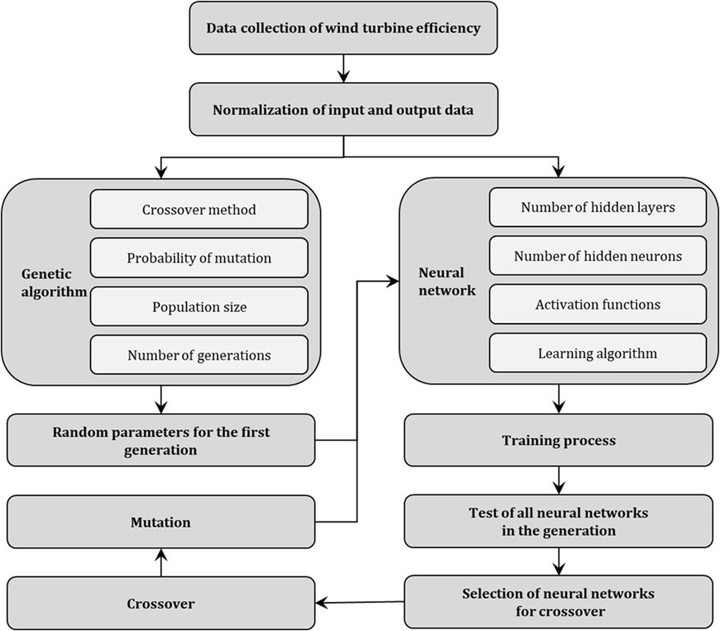
Figure 3. Genetic algorithm approach for optimizing neural network architecture.

In the research conducted, the parameters of the genetic algorithm were adopted with the values shown in Table 1. In each of the 50 generations, 25 neural networks are trained. Based on the evaluation of the trained neural networks in a given generation, the selection of five architectures with the smallest MSE error value for the test set is made. After the crossover of the selected networks on an individual to any basis using the intermediate recombination method with parameter d = 0.25 and mutation with probability p_mut = 0.1, a new generation of 25 models is formed. Due to computational complexity, a range of the number of neurons in the hidden layers was adopted from 1 to 30.

Table 1

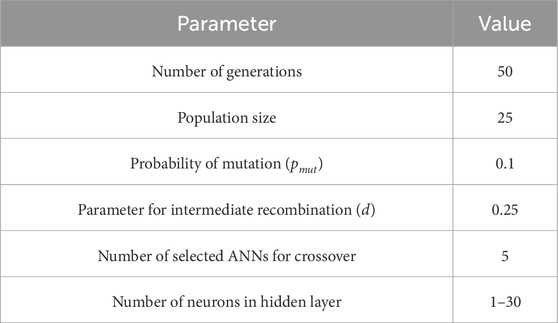
Table 1. Parameters for genetic algorithm.

Shapley Additive Explanations (SHAP) was used to determine the effect of individual MLP model input parameters on the predicted value of wind turbine power. The index ${\phi }_i$ denotes the SHAP value assigned to the i-th input parameter and represents its average contribution to the final model prediction. SHAP values are determined by the difference in the response of the predictive model depending on whether the feature is included or omitted in the model. In a formal sense, the value of ${\phi }_i$ is calculated according to Formula 12 (Cakiroglu et al., 2024):

${\phi }_i={\displaystyle \sum _{S\subseteq N\backslash \left\{i\right\}}}\frac{\left|S\right|!·\left(n-\left|S\right|-1\right)!}{n!}\left[f_{S\bigcup \left\{i\right\}}\left(x_{S\bigcup \left\{i\right\}}\right)-f_S\left(x_S\right)\right](13)$

where N is the set of all input parameters, n is the abundance of the N set, S is any subset of parameters not containing the i-th parameter, and $f_S\left(x_S\right)$ is the output value from the MLP based on the parameters in the S subset.

2.1.4 Accuracy evaluation methods

Assessing the precision of developed models is an important aspect of conducting research. Several measures and indicators are available in the literature to assess the degree of fit between the model and the empirical or estimated values. In this article, the evaluation of the fit of models based on artificial neural networks is carried out on the basis of the following four metrics Formulas 14–17:

— Mean Squared Error (MSE):

$MSE=\frac{1}{n}\sum _{i=1}^n{\left(y_i-y_{pred,i}\right)}^2,(14)$

— Root Mean Squared Error (RMSE):

$RMSE=\sqrt{\frac{1}{n}\sum _{i=1}^n{\left(y_i-y_{pred,i}\right)}^2},(15)$

— Mean Absolute Percentage Error (MAPE):

$MAPE=\frac{1}{n}\sum _{i=1}^n\left|\frac{y_i-y_{pred,i}}{y_i}\right|·100\%,(16)$

— Pearson correlation coefficient (R):

$R=\frac{{\sum }_{i=1}^n\left(y_i-\overline{y}\right)\left(y_{pred,i}-\overline{y_{pred}}\right)}{\sqrt{{\sum }_{i=1}^n{\left(y_i-\overline{y}\right)}^2{\sum }_{i=1}^n{\left(y_{pred,i}-\overline{y_{pred}}\right)}^2}}.(17)$

where $y_i$ denotes the i-th observed value of electricity production from the small wind turbine, $\overline{y}$ represents the mean of the observed values, $y_{pred,i}$ denotes the i-th predicted value, and $\overline{y_{pred}}$ represents the mean of the predicted values.

Evaluating model fit with a single measure is incomplete; for this reason MSE, RMSE, MAPE and Pearson’s correlation coefficient R have been proposed. MSE is used as a loss function for the learning process of feedforward regression neural networks, mainly because of its simple interpretation and differentiability. By rooting the MSE value, one gets the RMSE, which reflects the root mean square deviation of the model from the data. However, the MSE and RSME measures are sensitive to errors made for large values of the forecast variable, and they do not allow direct comparison with other neural models trained on other data sets. This problem can be solved by using the correlation coefficient R and the MAPE measure, which allow a unitless assessment of the model’s fit to empirical data, which implies the possibility of comparison with other models. However, in the case of MAPE, attention should be paid to its sensitivity to errors made with small values of the estimated variable, which is due to the denominator of the fraction that is a reference to these values (Christiansen et al., 2014; Li and Shi, 2010).

In the presented approach, the target variable (output variable of the MLP model) is the actual output power of the wind turbine, obtained from empirical operational data. The neural network model learns to represent the non-linear relationship between the input parameters (wind speed, turbine speed, temperature, wind direction) and the power generated by the turbine. In the MLP training process, the loss function was defined as the MSE, calculated between the predicted value and the actual power value. The RMSE value additionally allows the error to be interpreted in units of the dependent variable.

This approach unambiguously defines the context for the use of the presented algorithm in the regression task for SWT, allowing it to be applied to other locations and datasets as well, while keeping the same input structure and predictive objective.

2.2 Case study–small wind turbine

Experimental data was obtained from a small wind turbine with a nominal capacity of 12.0 kW, located in central Poland, which was the subject of the study and is described in more detail in the article (Zalewska et al., 2021). The specifications of the turbine are shown in Table 2.

Table 2

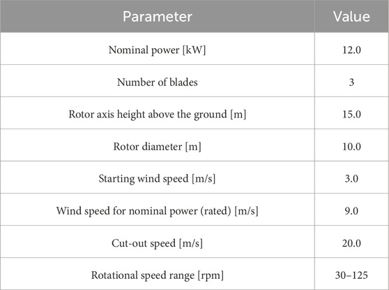
Table 2. Turbine specifications (data are from the turbine manufacturer).

2.2.1 Wind power

Metrological factors have a significant impact on wind power generation. The power generated by a wind turbine can be written using the Formula 18 (Olabi et al., 2021):

$P=\frac{1}{2}\rho A{V}^3(18)$

where: $\rho$ - air density [kg/m³], A–cross-sectional area of a turbine [m²], V - wind speed [m/s].

Of the listed components, wind speed has a major impact on wind turbine power output, as it varies with the cubic value of wind speed. Small differences in wind speed estimates result in significant differences in wind power estimates. Wind direction also affects power generation. However, compared to wind speed, it has less impact on the turbine power generated, since most turbines are designed to be properly oriented toward wind during operation (Singh et al., 2007). Furthermore, the power generated by a wind turbine depends on various design aspects, including the cut-in wind speed (the minimum wind speed required to start generating power), the rated wind speed (the speed at which the turbine reaches its rated power), and the cut-out wind speed (the maximum wind speed at which the turbine can generate power) (Carolin Mabel and Fernandez, 2008; Noorollahi et al., 2016). Wind power can also be affected by other factors, such as terrain, time of year, or time of day.

2.2.2 Database preprocessing

Many advantages can be found in performing nonlinear regression calculations, but the successful learning of a neural network is highly dependent on the quantity and quality of the data collected (Yan et al., 2019). To train and test the predictive model, data from an onshore small wind turbine with a nominal power of 12.0 kW, rotor diameter of 10.0 m and height of 15.0 m was used. The observation dataset contains information on the actual wind speed, turbine output power, rotor speed, wind direction, recording the occurrence of turbine failure or error. The collected parameters come from the Supervisory Control and Data Acquisition System (SCADA), which collects data from various sensors placed on the turbine. The recordings were recorded for 12 months, at a frequency of 1 min. The data set analyzed includes more than 500,000 raw data records. Furthermore, the data set was augmented with air temperature parameters recorded by a nearby metrological station from the Institute of Meteorology and Water Management.

The amount of collected data is considerable; however, there may be errors and outliers caused by the sensors or the data collection system. These include the occurrence of values outside the parameter range, missing data due to turbine availability, and electrical shutdowns. Periods of data loss due to machine failures, maintenance, and other circumstances are inevitable, so there was a need to apply data filtering (Zhang et al., 2019; Long et al., 2022). Before proceeding to the modeling stage, appropriate operations such as data cleaning and transformation were performed. The quality of the dataset was checked and cleaned. Subsequently, the data were filtered according to power-generating speed ranges, rotor speed ranges, absence of turbine failures, and errors. Turbine downtime and maintenance work were also taken into account. The wind speed range is from 0.0 to 15.0 m/s, as the turbine is stopped at wind speeds greater than 15.0 m/s. The wind power range is 0.0–12.0 kW, and the rotor speed range is 30–125 rpm. The wind direction parameters were converted to the sine of the wind direction for better illustration and the possibility of determining correlations with the other input data. Only data when the wind turbine is operating properly and generating power were selected for analysis. Figure 4 shows the output power of a small wind turbine during the study period.

Figure 4

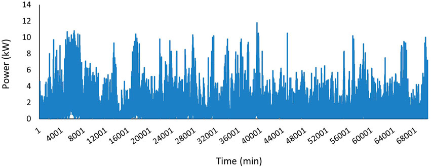
Figure 4. Power curve of a small wind turbine.

Input parameters for wind power generation forecasting were identified from the current state of the literature (Jamii et al., 2022; Liu et al., 2023; Sun et al., 2020) and selected: wind speed, rotor speed, wind direction and air temperature, while the output value is the wind power forecast value for the turbine. The selected data were analyzed for relationships between input and output parameters using Pearson’s correlation test. Wind speed and rotor speed (turbine speed) have a very good correlation with wind power production with a correlation value of 0.9 in both cases. For the direction of the wind and the temperature of the air, no clear correlation was identified (the correlation value is less than or equal to 0.1), indicating a weak relationship between the parameters studied.

Figure 5 shows the graphical relationships resulting from the study of correlations between input variables. Each dot plot in the grid represents a relationship between two variables, presenting them on horizontal and vertical axes in various combinations. This type of visualization is commonly used in statistical analysis because it captures both linear and non-linear relationships and potential anomalies in the data. It was noted that there is a strong positive correlation between turbine power and rotor speed, indicating that higher turbine speed results in higher power output. Positive correlations also exist between turbine power and wind speed, as well as between wind speed alone and turbine speed. Based on these observations, it can be concluded that wind speed and rotor speed are the key variables affecting the power generated by the turbine. Other variables, such as wind direction and temperature, appear to have limited impact on power generation in the data range studied.

Figure 5

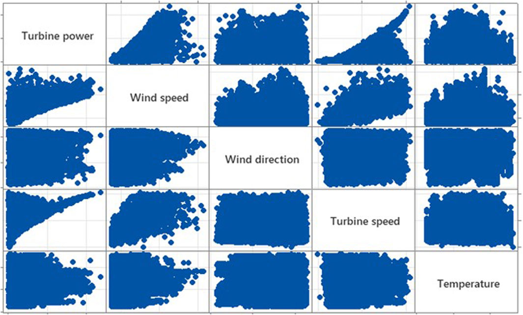
Figure 5. Correlation matrix diagram.

Correlation matrix diagram.Figure 5 shows the graphical relationships resulting from the study of correlations between input variables. Each dot plot in the grid represents a relationship between two variables, presenting them on horizontal and vertical axes in various combinations.. This chart provides a quick, quantitative comparison of the strength of the relationship between pairs of variables. It confirms previous observations - the highest correlation coefficients are between turbine power, wind speed and turbine speed. In contrast, the variables wind direction and temperature show low correlation with turbine power, confirming their limited usefulness as predictive features in further modeling. The use of both approaches - graphical and numerical - provides a complete picture of the interrelationships in the data set, which is an important step in the process of selecting input variables for the artificial neural network model.

Figure 6

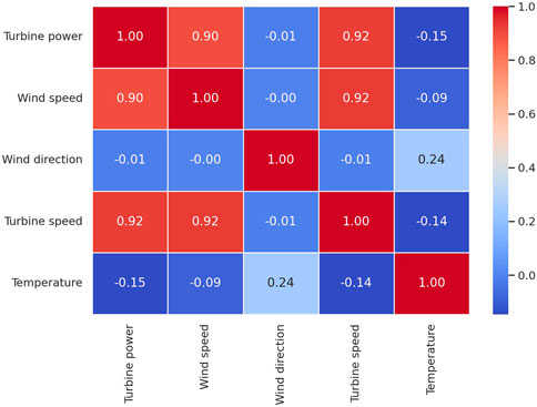
Figure 6. Heat map of correlations between input variables.

3 Results

3.1 Model development

The developed MLP models and GA were implemented in the MATLAB 2022b environment to predict electricity generation by a small wind turbine. Model training, testing, and validation were conducted using a workstation equipped with an Intel(R) Core(TM) i7-3970X CPU operating at 3.50 GHz and 16 GB of RAM.

The data was normalized before teaching the ANN model. After preprocessing the data, the ANN model was created. The preprocessed data were divided into a training data set, a validation data set and a test data set. Table 3 provides the characteristics and ranges of the variables used in the model, as well as the units of measurement for each variable.

Table 3

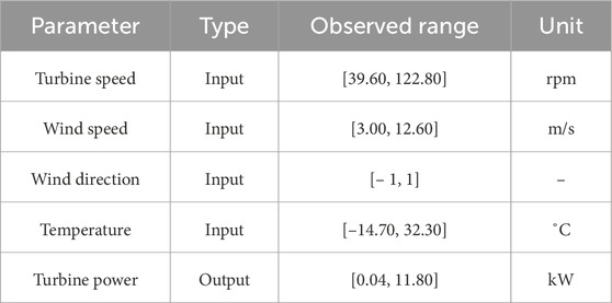
Table 3. Description of model parameters.

In the study carried out, 50 different neural network configurations (generations) were created, each with a varying number of neurons in the hidden layer. The results of the model adjustment, reflecting its performance during the training process, are shown in Figure 7. The graphs show the changes in MSE values as the generations progresses, allowing for an evaluation of the optimization process.

Figure 7

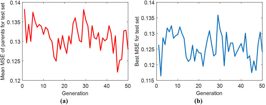
Figure 7. MSE values for the test set reached in GA optimization: (a) – mean for parents in each generation (5 selected best neural networks), (b) – best result in each generation.

Figure 7a shows a general trend of decreasing MSE in the initial generations, indicating progress in the optimization process. However, after a certain level is reached (around 0.125), the improvement becomes less noticeable, and the MSE values begin to fluctuate. In Figure 7b, a significant improvement in MSE can be seen at the beginning of the graph, suggesting that the algorithm quickly found better solutions. Then, as in graph (a), the values begin to fluctuate, which may suggest that a local minimum has been reached or that it is difficult to improve the results further. Both parts of the graphic suggest that optimization using the genetic algorithm significantly improved the model in the initial stages, resulting in lower MSE values for the test set. This indicates that the genetic algorithm effectively optimized the parameters of the neural network. The rapid decrease in MSE at the beginning is evidence that GA helped find better model configurations. However, the stochastic nature of initializing the initial weights of the MLP model and the random division of the set into training, validation, and test subsets imply a nonmonotonic course of the optimization objective function for the best solutions achieved in successive iterations of the genetic algorithm.

Table 4 shows the optimal architecture of the multilayer neural network obtained during the optimization process. It details the number of neurons in each hidden layer and the activation functions used. The MLP architecture is characterized by a significant variation in the number of neurons in each hidden layer. This selection of the number of neurons suggests careful adaptation of the model to the specific data set in order to balance the ability to learn with the risk of overlearning. The variety of activation functions used indicates the specific needs of the data, which require an unusual approach to neural network design to achieve optimal results.

Table 4

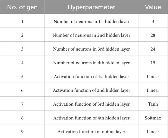
Table 4. Optimal architecture of MLP.

Based on Equations 14–17, prediction errors were calculated for neural networks in all data sets. The results of these calculations are presented in Table 5.

Table 5

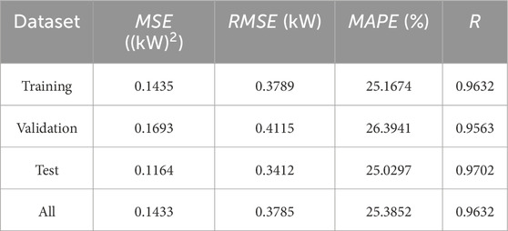
Table 5. Results for the optimal MLP model.

The model achieves high accuracy on the training, validation, and test sets, indicating its ability to learn efficiently from training data and its good generalization to new data. The MSE and RMSE values are relatively low on each of the data sets, indicating good quality predictions. In particular, the low MSE = 0.1164 (kW)² i RMSE = 0.3412 kW in the test set underscore the effectiveness in predicting real data. The MAPE value, oscillating around 25% for all sets, suggests that the model has some level of percentage error in the forecasts, but this is relatively stable between data sets and consequently indicates consistency in model performance. It should be noted, however, that MAPE is sensitive to low values of the forecast variable, which can lead to overestimation of percentage errors in such cases. The high correlation coefficient R values above 0.95 for all data sets suggest a strong correlation between the forecasted and actual values. In particular, the value of R = 0.97 for the test set indicates that the model reproduces the correlations in the test data very well, indicating its high quality and effectiveness in the prediction. The comparison of results in the validation and test sets indicates the stability of the model, which is crucial for its usefulness in real-world applications. The differences in metrics between the sets are small, suggesting that the model is not overtrained. It can be concluded that the MLP model is well calibrated and shows satisfactory accuracy and stability in different data sets, making it a robust tool for forecasting in a given context.

Figure 8 presents four regression graphs that illustrate the MLP model’s prediction performance for the training, validation, test and total prediction data sets. These graphs juxtapose the model’s predicted output values with the experimental results, showing the accuracy of the model’s fit to the actual data.

Figure 8

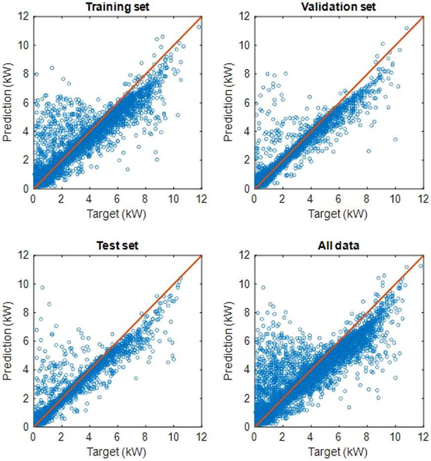
Figure 8. Results for training, validation, and test of the MLP model.

On each graph, there is an orange line that indicates a perfect fit, where the predicted value equals the actual value (Prediction = Target). The points on this line represent perfect predictions of the model. Points close to this line in each graph indicate good agreement between predictions and actual values, suggesting that the model predicts outcomes well. The graph in the validation set shows a similar distribution to that for the training set, but the spread of points around the line defining the perfect fit is slightly larger. This suggests that the model generalizes well but is slightly less precise on the new, previously unseen data. The distribution of points on the graph in the test set is similar to the other sets, with some scatter especially at higher power values. This indicates that the model maintains its performance on the test data, but accuracy may be limited for higher values. The graph for the entire dataset is similar to the other graphs, indicating the model consistency across different evaluation phases.

The density of points, near the line defining a perfect fit, in the graphs for the training, validation, and test sets suggests that the model has robust predictive ability across the different evaluation phases. The apparent scatter, especially for higher values, indicates the possible difficulty of the model in accurately predicting extreme power values. The greater the scatter, the greater the error in the prediction. This may suggest that the model has generalization problems in these areas and could require further optimization, such as by tuning the parameters or using more training data in these ranges. Significant deviations from the ideal line in certain ranges could also indicate data quality problems in these ranges, such as noise or measurement errors. A comparison of the graphs for the training, validation, and test sets reveals no significant differences in the distribution of scores. This indicates that the model is well tuned and has not overfitted (not over-fitted to the training data). The graphs show a relatively good fit of the scoring plot data, indicating a well-designed model.

In the graph shown in Figure 9, one can observe the course of change of the MSE as a function of the number of epochs for the training, validation and test sets. There is a sharp drop in the error after the first few epochs, which then stabilizes at a low level, indicating that the model has been successfully learned. The errors on all three sets are very close to each other, confirming the absence of significant signs of overfitting. This course of action confirms the correct learning process of the model and the good overall quality of the fit.

Figure 9

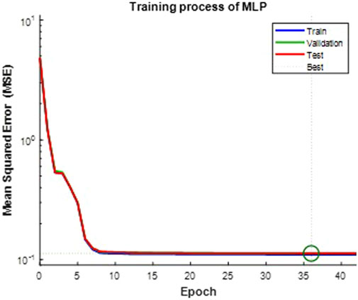
Figure 9. Training process of developed MLP.

3.2 Sensitivity analysis

Sensitivity analysis in neural networks is carried out to determine how individual input parameters affect the output value of the model, in the case of the proposed approach - the power of the turbine. In this way, it is possible to identify the risks associated with the availability and performance degradation of the system (Tang et al., 2024). The developed model was subjected to a sensitivity analysis regarding the dependence of turbine power on wind speed and the sine of the wind angle, assuming a constant turbine speed of 65.5 (rpm). Sensitivity analysis was carried out separately for five variants with different air temperatures (from −10.0°C to 30.0°C). The results are shown in Figure 10. The color of the spectrum in the graphs and response plots represents the interaction between wind speed, wind angle sine, and generated turbine power.

Figure 10

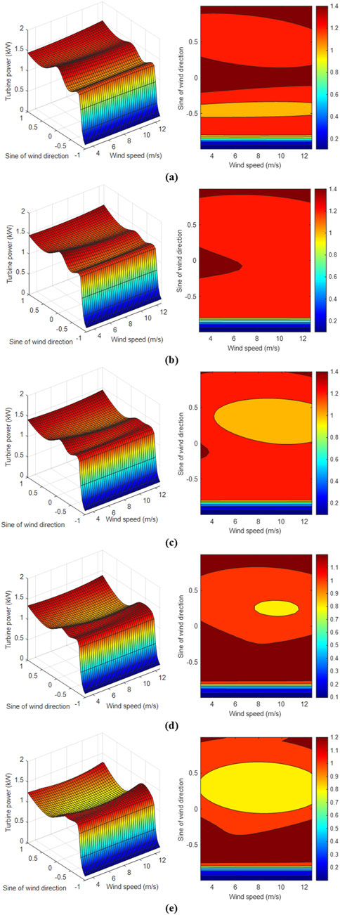
Figure 10. Sensitivity analysis for a sine of wind direction of 0 and: (a) temperature = −10.0°C, (b) temperature = 0.0°C, (c) temperature = 10.0°C, (d) temperature = 20.0°C, (e) temperature = 30.0°C.

An analysis of the charts shows that under these assumptions, wind speed has little effect on turbine power. Turbine power remains relatively constant throughout the range of wind speeds shown in the charts. Power variations depend mainly on the sine of the wind direction angle. The highest turbine power (about 1.5 kW) in all the variants presented is achieved when the sine is equal to 1 (90.0°). This means that the turbine operates most efficiently when the wind blows perpendicular to the turbine blades. However, when the sine of the wind direction is equal to −1 (270.0°) and the wind blows perpendicularly from the back of the turbine, the turbine does not generate power. Wind from this direction cannot effectively drive the blades, so the power generated by the turbine is very low or zero, regardless of the wind speed. Temperature seems to have little effect on the overall shape of the relationship. However, it can gently affect turbine power values under given conditions of wind speed and direction. For example, at lower air temperatures, the turbine may generate slightly higher power at the same wind speeds compared to higher temperatures. This may indicate changes in air density with temperature. At lower temperatures, the air is denser, increasing the mass of air flowing through the turbine and may consequently increase its power output. The graphs shown, assuming a turbine speed of 65.5 (rpm), show that it is mainly the wind direction (expressed as the sine of the wind direction angle) that determines the power generated by the turbine, rather than the wind speed itself.

The effect of temperature and wind speed on turbine output can vary from season to season. Using the data from this analysis can help predict and plan energy production in different seasons. Increases in temperature can slightly affect power output, which is important for planning turbine locations and optimizing turbine performance. These results can be useful for optimizing wind turbine settings, especially in regions with varying climatic conditions.

Figure 11 shows 3D sensitivity analysis plots of turbine power output as a function of turbine speed (turbine speed) and wind speed, assuming the sine of the wind direction angle is 0 (which means that the wind blows parallel to the turbine axis).

Figure 11

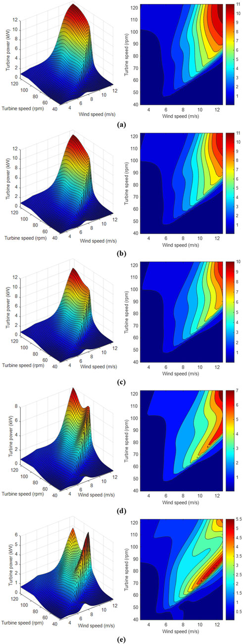
Figure 11. Sensitivity analysis for a turbine speed of 65.5 (rpm) and: (a) temperature = −10.0°C, (b) temperature = 0.0°C, (c) temperature = 10.0°C, (d) temperature = 20.0°C, (e) temperature = 30.0°C.

Each graph shows a clear peak in power, which shifts as the temperature changes. This suggests that the optimal turbine speed also depends on the ambient temperature. At lower temperatures, such as −10.0°C (a) and 0.0°C (b), the achievable turbine power is higher compared to higher temperatures, such as 20.0°C (d) and 30.0°C (e). The most efficient turbine operation, with a maximum power output of approximately 12.0 kW, occurs at −10.0°C and is achieved at a turbine speed of 120 rpm and a wind speed of 12.0 m/s. This indicates the optimal turbine operating conditions that provide the highest output. In all the graphs, at low wind speeds below 6.0 m/s, the turbine output is very low, regardless of the turbine speed. Similarly, at turbine speeds below 60 rpm, turbine output is also low, regardless of wind speed. This perfectly confirms the technical conditions of the turbine: a minimum wind speed is required for effective operation and a minimum turbine speed is required.

The graphs show that as the air temperature increases, the maximum achievable power of the turbine decreases. This means that the system operates more efficiently at lower temperatures with the assumed wind angle. Higher temperatures can adversely affect turbine stability and efficiency. A general characteristic that can be observed is that the power output of the turbine increases with increasing wind speed and turbine speed. Knowing at what operating parameters (wind speed and turbine speed) maximum power can be achieved is crucial to optimizing turbine performance, minimizing costs, and maximizing energy production. This analysis suggests that for maximum energy efficiency, changes in temperature conditions should be taken into account and the turbine’s operating parameters should be adjusted to accommodate these changes. This can help optimize wind turbine operation, especially under changing climatic conditions.

In order to increase the interpretability of the trained neural network model, SHAP analysis was performed. The results in Figure 12 show that turbine speed had the greatest impact on predicted power, followed by air temperature and wind speed. The result with temperature may seem contradictory to initial observations (e.g., low linear correlation), but it is important to remember that SHAP analysis takes into account non-linear and complex interactions between features in models such as MLPs. The influence of temperature can be indirect, such as by affecting air density and thus energy production efficiency, which could have been captured by the neural network. Thus, the model is able to extract relationships that are not directly apparent with simple statistical analyses. Wind direction showed a minimal, slightly negative effect on the predictions. This may be due to the limited variation of this variable in the analyzed geographic area or its indirect influence through other variables. SHAP analysis confirms that the model’s predictions are consistent with the actual physical relationships occurring in the energy production process of small wind turbines.

Figure 12

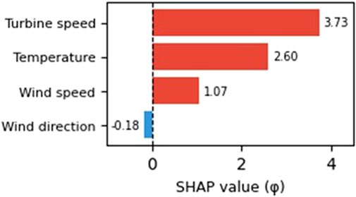
Figure 12. SHAP value for the developed model.

4 Discussion and conclusion

The simplest way to harness wind energy is to convert it to electricity using a wind turbine and connect it to the power grid. However, the stability of the supply is strongly affected by the stochastic nature of the wind. To solve this challenge, it is necessary to develop appropriate models to generate accurate forecasts of wind speed and power. The use of wind power forecasting technology is an effective tool to provide technical support for the safety, stability, and economic operation of wind turbines. However, wind power forecasting involves a certain degree of uncertainty due to the instability of wind speeds and fluctuations in wind turbine output. From a technical point of view, it is difficult to increase the precision of wind turbine power forecasts. However, existing technologies can help better understand these uncertainties and improve power system performance.

This study demonstrates the potential of advanced machine learning methods in the wind energy industry. The complexity of the industry’s systems is constantly increasing, and the methods and algorithms to ensure their performance are becoming more reliable due to the growing amount of data and variety of variables. The study uses artificial neural networks to develop a model to forecast the output of small wind turbines. The paper presents an optimized output power simulation method and effective training of MLP neural networks. The results of this study have significantly improved the simulation and precision of power prediction. Neural networks show utility in various applications and can be integrated with other methods to optimize their performance with hybrid systems. This article can be a valuable resource for those interested in effective tools in the rapidly growing field of wind turbines.

Artificial neural networks, thanks to their strengths, make it possible to make high-precision predictions, even though they are based on general, often averaged data. They also stand out for their high flexibility, both in terms of the data they rely on and the information they can provide. In addition, its important feature is the ability to quickly adapt the model to power plants with different technical parameters. It is also worth noting that the accuracy of the model is highly dependent on the quantity and quality of the input data provided.

The created MLP network showed high quality in the learning, testing, and validation processes, achieving results in the range of 0.96–0.97. In addition, a prediction error analysis was carried out to compare the predicted values with the actual data. The MSE, RMSE and MAPE measures confirmed that the accuracy of the predictions obtained by the prediction models used is satisfactory. The neural network model provides reliable predictions of the output power generated by the wind turbine based on input parameters such as wind speed, rotor speed, wind direction, and air temperature. Wind speed was shown to be the variable that most influences the output of wind turbine power.

The results of the analyzes indicate that the MLP model shows good agreement between predictions and actual values, especially in the range of moderate values of turbine power. Analyzing Figure 8, it was observed that most points in the graphs are close to the baseline, indicating that the model is well adapted to the data used for training and testing. However, there is potential to further optimize the model by further tuning the parameters, using more training data, or applying more advanced modeling techniques.

Sensitivity analysis has provided a better understanding of the impact of various factors on the performance of a small wind turbine. Information about the impact of weather conditions on turbine efficiency can be used to optimize operating costs, such as scheduling service and maintenance more precisely during periods of lower expected output and developing contingency strategies to minimize downtime and equipment damage. The results of the analysis can also influence decisions on turbine design and wind farm site selection, such as adapting turbine technology to specific climatic conditions or investing in locations where higher efficiency is anticipated. Furthermore, the results can point to directions for further research and development of wind turbine technology, which can lead to innovations that increase the efficiency and reliability of energy systems.

One of the key factors affecting the effectiveness of forecasting energy production by small wind turbines is geographic location and the associated regional nature of wind conditions. This study used data from a single turbine located in central Poland, meaning that the model was fitted to a moderate and relatively stable wind profile typical of the inland part of the country. Such a range of data may not be sufficient to directly generalize the results to other regions, where wind characteristics can vary significantly. For example, coastal regions are often characterized by higher average wind speeds and a more predictable diurnal rhythm, while mountainous areas are characterized by high variability and turbulent phenomena. These variables can significantly affect the structure of the input data used in the neural model. However, it should be emphasized that the model proposed in the paper is universal in nature. The developed algorithm can be adapted to other locations by re-training the model on area-specific data. As a result, the approach can be applied to different climatic and geographic conditions, while maintaining the same model structure and predictive methodology. This means that despite the local nature of the source data, the methodology has the potential to be generalized and can be effectively implemented in other operational contexts for small wind turbines.

The accuracy of the prediction can be affected by many additional dependencies, these include information on the wind turbine’s environment, the unit’s operating status, recorded historical data, and weather conditions. The performance of a prediction model will vary from one wind turbine model to another to account for the varying characteristics and layouts of the turbines. Therefore, it is important to understand the factors that affect the prediction error, which may be, for example, the accuracy of the input data, the design of the wind turbine system, or the probability of component failure. In addition, wind power is significantly characterized by location dependence and distribution heterogeneity for different locations.

The predictive model presented here uses operational data including variables such as wind speed, wind direction, air temperature and turbine speed. The model was developed based on historical data from a specific period of the turbine’s operation, without direct consideration of factors related to the turbine’s aging or cyclic maintenance. In operational practice, wind turbines are subject to gradual technical degradation resulting from, among other things, wear of mechanical components, material fatigue, contamination, or deterioration of blade aerodynamic characteristics. Such changes can result in a gradual reduction in the efficiency of converting wind energy into electricity. Moreover, irregular maintenance or lack of maintenance can accelerate this process and affect the variability of the turbine’s performance, which in the long term translates into greater discrepancies between projected and actual energy production. The lack of inclusion of variables describing the age of the turbine, the number of maintenance inspections performed, the history of faults or the duration of uninterrupted operation limits the model’s ability to capture long-term degradation trends.

The energy production predicted for a wind turbine using the SSN model is in good agreement with the actual values. The results obtained prove the effectiveness of using MLP-type neural networks for the task of forecasting the energy production of small wind turbines. The model can be useful for energy planners and wind turbine owners in planning and implementing future activities. Finally, it was concluded that the presented forecasting model is suitable for wind energy forecasting. This study is innovative, practical and has great potential, as the proposed model can also be successfully applied to forecasting other renewable energy sources.

In the next stages of the study, the authors will focus on verifying the energy efficiency of small wind turbines. It will be crucial to verify the simulation models as closely as possible to real operating conditions. This can contribute to improving forecasting accuracy and optimizing SWT designs.

Data availability statement

The original contributions presented in the study are included in the article/supplementary material, further inquiries can be directed to the corresponding author.

Author contributions

JZ-L: Conceptualization, Data curation, Formal Analysis, Investigation, Methodology, Resources, Software, Validation, Visualization, Writing – original draft, Writing – review and editing. MO: Formal Analysis, Methodology, Software, Visualization, Writing – original draft. JM: Conceptualization, Formal Analysis, Funding acquisition, Project administration, Supervision, Visualization, Writing – review and editing.

Funding

The author(s) declare that financial support was received for the research and/or publication of this article. The authors acknowledge the Military University of Technology for the financial support (research project UGB 000007-W100-22) in this study.

Conflict of interest

The authors declare that the research was conducted in the absence of any commercial or financial relationships that could be construed as a potential conflict of interest.

Generative AI statement

The author(s) declare that no Generative AI was used in the creation of this manuscript.

Publisher’s note

All claims expressed in this article are solely those of the authors and do not necessarily represent those of their affiliated organizations, or those of the publisher, the editors and the reviewers. Any product that may be evaluated in this article, or claim that may be made by its manufacturer, is not guaranteed or endorsed by the publisher.

References

Ak, R., Li, Y. F., Vitelli, V., and Zio, E. (2018). Adequacy assessment of a wind-integrated system using neural network-based interval predictions of wind power generation and load. Int. J. Electr. Power and Energy Syst. 95, 213–226. doi:10.1016/J.IJEPES.2017.08.012

CrossRef Full Text | Google Scholar

Al-Ghamdi, A.-B., Kamel, S., and Khayyat, M. (2021). Evaluation of artificial neural networks performance using various normalization methods for water demand forecasting. 2021 Natl. Comput. Coll. Conf. (NCCC), 1–6. doi:10.1109/NCCC49330.2021.9428856

CrossRef Full Text | Google Scholar

Al-Naser, M., Elshafei, M., and Al-Sarkhi, A. (2016). Artificial neural network application for multiphase flow patterns detection: a new approach. J. Petroleum Sci. Eng. 145, 548–564. doi:10.1016/J.PETROL.2016.06.029

CrossRef Full Text | Google Scholar

Augustyn, A., and Kamiński, J. (2018). A review of methods applied for wind power generation forecasting. Polityka Energetyczna - Energy Policy J. 21 (2), 139–150. doi:10.33223/epj/96214

CrossRef Full Text | Google Scholar

Babbar, S. M., and Langah, T. H. (2022). Wind power prediction using neural networks with different training models. Indonesian J. Innovation Appl. Sci. (IJIAS) 2 (1), 12–17. doi:10.47540/IJIAS.V2I1.340

CrossRef Full Text | Google Scholar

Bircanoglu, C., and Arica, N. (2018). A comparison of activation functions in artificial neural networks. 26th Signal Process. Commun. Appl. Conf. (SIU), 1–4. doi:10.1109/SIU.2018.8404724

CrossRef Full Text | Google Scholar

Blonbou, R. (2011). Very short-term wind power forecasting with neural networks and adaptive Bayesian learning. Renew. Energy 36 (3), 1118–1124. doi:10.1016/J.RENENE.2010.08.026

CrossRef Full Text | Google Scholar

Cakiroglu, C., Demir, S., Hakan Ozdemir, M., Latif Aylak, B., Sariisik, G., and Abualigah, L. (2024). Data-driven interpretable ensemble learning methods for the prediction of wind turbine power incorporating SHAP analysis. Expert Syst. Appl. 237, 121464. doi:10.1016/J.ESWA.2023.121464

CrossRef Full Text | Google Scholar

Carolin Mabel, M., and Fernandez, E. (2008). Analysis of wind power generation and prediction using ANN: a case study. Renew. Energy 33 (5), 986–992. doi:10.1016/J.RENENE.2007.06.013

CrossRef Full Text | Google Scholar

Chia, M. Y., Huang, Y. F., and Koo, C. H. (2022). “ANN-based reference evapotranspiration estimation: effects of data normalization and parameters selection,” in Proceedings of international conference on emerging technologies and intelligent systems (Springer Science and Business Media Deutschland GmbH), 3–12. doi:10.1007/978-3-030-85990-9_1/COVER

CrossRef Full Text | Google Scholar

Christiansen, N. H., Voie, P. E. T., Winther, O., and Høgsberg, J. (2014). Comparison of neural network error measures for simulation of slender marine structures. J. Appl. Math. 2014, 1–11. doi:10.1155/2014/759834

CrossRef Full Text | Google Scholar

Consilium (2023). European parliament and Council of the European union. Available online at: https://www.consilium.europa.eu/pl/press/press-releases/2023/03/30/council-and-parliament-reach-provisional-deal-on-renewable-energy-directive/ (Accessed May 25, 2024).

Google Scholar

Drałus, G., and Gomółka, Z. (2017). Prognozowanie produkcji energii elektrycznej w systemach fotowoltaicznych. Acta Scientifica Academiae Ostroviensis. Sectio A, Nauki Humanistyczne. Społeczne i Tech. 9 (1), 285–296.

Google Scholar

Eltayesh, A., Castellani, F., Natili, F., Burlando, M., and Khedr, A. (2023). Aerodynamic upgrades of a Darrieus vertical axis small wind turbine. Energy Sustain. Dev. 73, 126–143. doi:10.1016/J.ESD.2023.01.018

CrossRef Full Text | Google Scholar

European sources (2023). Directive of the European Parliament and of the Council on promoting the use of energy from renewable sources. The European Parliament And The Council Of The European Union. Available online at: https://eur-lex.europa.eu/eli/dir/2023/2413/oj

Google Scholar

Foley, A. M., Leahy, P. G., Marvuglia, A., and McKeogh, E. J. (2012). Current methods and advances in forecasting of wind power generation. Renew. Energy 37 (1), 1–8. doi:10.1016/j.renene.2011.05.033

CrossRef Full Text | Google Scholar

Garud, K. S., Jayaraj, S., and Lee, M. Y. (2021). A review on modeling of solar photovoltaic systems using artificial neural networks, fuzzy logic, genetic algorithm and hybrid models. Int. J. Energy Res. 45 (1), 6–35. doi:10.1002/ER.5608

CrossRef Full Text | Google Scholar

Global Wind Energy Council (2023). Global wind report 2023. Brussels. Available online at: https://gwec.net/wp-content/uploads/2023/04/GWEC-2023_interactive.pdf (Accessed May 12, 2024).

Google Scholar

Gómez, C. Q. M., and García, F. P. M. (2018). Wind energy power prospective. Renew. Energies, 83–95. doi:10.1007/978-3-319-45364-4_6

CrossRef Full Text | Google Scholar

Gómez, C. Q. M., García, F. P. M., Arcos, A. J., Cheng, L., Kogia, M., Mohimi, A., et al. (2017). A heuristic method for detecting and locating faults employing electromagnetic acoustic transducers. Eksploat. i Niezawodn. 19 (4), 493–500. doi:10.17531/EIN.2017.4.1

CrossRef Full Text | Google Scholar

Han, Y., Mi, L., Shen, L., Cai, C., Liu, Y., Li, K., et al. (2022). A short-term wind speed prediction method utilizing novel hybrid deep learning algorithms to correct numerical weather forecasting. Appl. Energy 312, 118777. doi:10.1016/J.APENERGY.2022.118777

CrossRef Full Text | Google Scholar

Henderi, H. (2021). Comparison of min-max normalization and Z-score normalization in the K-nearest neighbor (kNN) algorithm to test the accuracy of types of breast cancer. IJIIS Int. J. Inf. Inf. Syst. 4 (1), 13–20. doi:10.47738/IJIIS.V4I1.73

CrossRef Full Text | Google Scholar

Heng, J., Hong, Y., Hu, J., and Wang, S. (2022). Probabilistic and deterministic wind speed forecasting based on non-parametric approaches and wind characteristics information. Appl. Energy 306, 118029. doi:10.1016/J.APENERGY.2021.118029

CrossRef Full Text | Google Scholar

Hossa, T., Sokołowska, W., Fabisz, K., and Filipowska, A. (2014). Prognozowanie generacji wiatrowej z wykorzystaniem metod lokalnych i regresji nieliniowej. Rynek Energii 2, 61–68.

Google Scholar

IEAIRENAUNSD (2022). Tracking SDG 7: the energy progress report. Washington DC. Available online at: www.worldbank.org (Accessed December 15, 2023).

Google Scholar

Jamii, J., Mansouri, M., Trabelsi, M., Mimouni, M. F., and Shatanawi, W. (2022). Effective artificial neural network-based wind power generation and load demand forecasting for optimum energy management. Front. Energy Res. 10, 898413. doi:10.3389/FENRG.2022.898413

CrossRef Full Text | Google Scholar

Jiménez, A. A., Muñoz, C. Q. G., and Márquez, F. P. G. (2018). Machine learning for wind turbine blades maintenance management. Energies 11 (1), 13. doi:10.3390/EN11010013

CrossRef Full Text | Google Scholar

Jóźwiak, A., and Lesiak, G. (2020). “Analysis and prediction of security factors in public passenger transport using artificial neural networks,” in 35th ibima conference - education excellence and innovation management: a 2025 vision to sustain economic development during global challenges (Seville, Spain), 11242–11254.

Google Scholar

Jung, J., and Broadwater, R. P. (2014). Current status and future advances for wind speed and power forecasting. Renew. Sustain. Energy Rev. 31, 762–777. doi:10.1016/J.RSER.2013.12.054

CrossRef Full Text | Google Scholar

Karaman, Ö. A. (2023). Prediction of wind power with machine learning models. Appl. Sci. 13 (20), 11455. doi:10.3390/APP132011455

CrossRef Full Text | Google Scholar

Kim, J. H., and Powell, W. B. (2011). Optimal energy commitments with storage and intermittent supply. Operations Res. 59 (6), 1347–1360. doi:10.1287/OPRE.1110.0971

CrossRef Full Text | Google Scholar

Kou, P., Gao, F., and Guan, X. (2013). Sparse online warped Gaussian process for wind power probabilistic forecasting. Appl. Energy 108, 410–428. doi:10.1016/J.APENERGY.2013.03.038

CrossRef Full Text | Google Scholar

Kurdi, M. (2019). An effective genetic algorithm with a critical-path-guided Giffler and Thompson crossover operator for job shop scheduling problem. Int. J. Intelligent Syst. Appl. Eng. 7 (1), 13–18. doi:10.18201/ijisae.2019751247

CrossRef Full Text | Google Scholar

Li, G., and Shi, J. (2010). On comparing three artificial neural networks for wind speed forecasting. Appl. Energy 87 (7), 2313–2320. doi:10.1016/J.APENERGY.2009.12.013

CrossRef Full Text | Google Scholar

Li, Y., Wang, R., Li, Y., Zhang, M., and Long, C. (2023). Wind power forecasting considering data privacy protection: a federated deep reinforcement learning approach. Appl. Energy 329, 120291. doi:10.1016/J.APENERGY.2022.120291

CrossRef Full Text | Google Scholar

Liu, H., Yu, C., Wu, H., Duan, Z., and Yan, G. (2020a). A new hybrid ensemble deep reinforcement learning model for wind speed short term forecasting. Energy 202, 117794. doi:10.1016/J.ENERGY.2020.117794

CrossRef Full Text | Google Scholar

Liu, M., Cao, Z., Zhang, J., Wang, L., Huang, C., and Luo, X. (2020b). Short-term wind speed forecasting based on the Jaya-SVM model. Int. J. Electr. Power and Energy Syst. 121, 106056. doi:10.1016/J.IJEPES.2020.106056

CrossRef Full Text | Google Scholar

Liu, Y., He, J., Wang, Y., Liu, Z., and He, L. (2023). Short-term wind power prediction based on CEEMDAN-SE and bidirectional LSTM neural network with Markov chain. Energies 16 (14), 5476. doi:10.3390/EN16145476

CrossRef Full Text | Google Scholar

Liu, Y., Qin, H., Zhang, Z., Pei, S., Jiang, Z., Feng, Z., et al. (2020c). Probabilistic spatiotemporal wind speed forecasting based on a variational Bayesian deep learning model. Appl. Energy 260, 114259. doi:10.1016/J.APENERGY.2019.114259

CrossRef Full Text | Google Scholar

Long, H., Xu, S., and Gu, W. (2022). An abnormal wind turbine data cleaning algorithm based on color space conversion and image feature detection. Appl. Energy 311, 118594. doi:10.1016/J.APENERGY.2022.118594

CrossRef Full Text | Google Scholar

Luo, X. J., Oyedele, L. O., Ajayi, A. O., Akinade, O. O., Owolabi, H. A., and Ahmed, A. (2020). Feature extraction and genetic algorithm enhanced adaptive deep neural network for energy consumption prediction in buildings. Renew. Sustain. Energy Rev. 131, 109980. doi:10.1016/J.RSER.2020.109980

CrossRef Full Text | Google Scholar

Markowicz, K. (2011). Pomiary oraz analiza pola wiatru dla potrzeb energetycznych. Available online at: https://www.igf.fuw.edu.pl/∼kmark/stacja/wyklady/EnergiaOdnawialna/Wiatr/AnalizaZasobowWiatru.pdf (Accessed March 23, 2023).

Google Scholar

Marugán, A. P., Márquez, F. P. G., Perez, J. M. P., and Ruiz-Hernández, D. (2018). A survey of artificial neural network in wind energy systems. Appl. Energy 228, 1822–1836. doi:10.1016/J.APENERGY.2018.07.084

CrossRef Full Text | Google Scholar

Mentes, S., Tan, E., Özdemir, T., Unal, E., Unal, Y., Efe, B., et al. (2012). “Short term wind power forecast in manisa, Turkey by using the WRF model coupled to a CFD model,” in EWRES and ECRES the European workshop and conference on renewable energy systems (Antalya).

Google Scholar

Nielson, J., Bhaganagar, K., Meka, R., and Alaeddini, A. (2020). Using atmospheric inputs for Artificial Neural Networks to improve wind turbine power prediction. Energy 190, 116273. doi:10.1016/J.ENERGY.2019.116273

CrossRef Full Text | Google Scholar

Noorollahi, Y., Jokar, M. A., and Kalhor, A. (2016). Using artificial neural networks for temporal and spatial wind speed forecasting in Iran. Energy Convers. Manag. 115, 17–25. doi:10.1016/J.ENCONMAN.2016.02.041

CrossRef Full Text | Google Scholar

Okumus, I., and Dinler, A. (2016). Current status of wind energy forecasting and a hybrid method for hourly predictions. Energy Convers. Manag. 123, 362–371. doi:10.1016/J.ENCONMAN.2016.06.053

CrossRef Full Text | Google Scholar

Olabi, A. G., Wilberforce, T., Elsaid, K., Salameh, T., Sayed, E. T., Husain, K. S., et al. (2021). Selection guidelines for wind energy technologies. Energies 14 (11), 3244. doi:10.3390/EN14113244

CrossRef Full Text | Google Scholar

Özgür, M. A. (2014). ANN-based evaluation of wind power generation: a case study in Kutahya, Turkey. J. Energy South. Afr. 25 (4), 11–22. doi:10.17159/2413-3051/2014/V25I4A2233

CrossRef Full Text | Google Scholar

Popławski, T., Szeląg, P., Całus, D., Głowiński, C., and Adamowicz, Ł. (2013). Użycie metod grupowania do prognozowania generacji wiatrowej. Rynek Energii 5 (108).

Google Scholar

Pourmousavi Kani, S. A., and Ardehali, M. M. (2011). Very short-term wind speed prediction: a new artificial neural network–Markov chain model. Energy Convers. Manag. 52 (1), 738–745. doi:10.1016/J.ENCONMAN.2010.07.053

CrossRef Full Text | Google Scholar

Qureshi, S., Shaikh, F., Kumar, L., Ali, F., Awais, M., and Gürel, A. E. (2023). Short-term forecasting of wind power generation using artificial intelligence. Environ. Challenges 11, 100722. doi:10.1016/J.ENVC.2023.100722

CrossRef Full Text | Google Scholar

Rahman, M. M., Shakeri, M., Tiong, S. K., Khatun, F., Amin, N., Pasupuleti, J., et al. (2021). Prospective methodologies in hybrid renewable energy systems for energy prediction using artificial neural networks. Sustainability 13 (4), 2393. doi:10.3390/SU13042393

CrossRef Full Text | Google Scholar

Senthil Kumar, P. (2019). Improved prediction of wind speed using machine learning. EAI Endorsed Trans. Energy Web 6 (23), 157033. doi:10.4108/EAI.13-7-2018.157033

CrossRef Full Text | Google Scholar

Severiano, C. A., Cândido, L. S. P., Weiss, C. M., and Gadelha, G. F. (2021). Evolving fuzzy time series for spatio-temporal forecasting in renewable energy systems. Renew. Energy 171, 764–783. doi:10.1016/J.RENENE.2021.02.117

CrossRef Full Text | Google Scholar

Singh, S., Bhatti, T. S., and Kothari, D. P. (2007). Wind power estimation using artificial neural network. J. Energy Eng. 133 (1), 46–52. doi:10.1061/(ASCE)0733-9402(2007)133:1(46)

CrossRef Full Text | Google Scholar

Sun, H., Qiu, C., Lu, L., Gao, X., Chen, J., and Yang, H. (2020). Wind turbine power modelling and optimization using artificial neural network with wind field experimental data. Appl. Energy 280, 115880. doi:10.1016/J.APENERGY.2020.115880

CrossRef Full Text | Google Scholar

Sweeney, C., Bessa, R. J., Browell, J., and Pinson, P. (2020). The future of forecasting for renewable energy. Wiley Interdiscip. Rev. Energy Environ. 9 (2), e365. doi:10.1002/WENE.365

CrossRef Full Text | Google Scholar

Taghinezhad, J., and Sheidaei, S. (2022). Prediction of operating parameters and output power of ducted wind turbine using artificial neural networks. Energy Rep. 8, 3085–3095. doi:10.1016/J.EGYR.2022.02.065

CrossRef Full Text | Google Scholar

Tajmiri, S., Azimi, E., Hosseini, M. R., and Azimi, Y. (2020). Evolving multilayer perceptron, and factorial design for modelling and optimization of dye decomposition by bio-synthetized nano CdS-diatomite composite. Environ. Res. 182, 108997. doi:10.1016/J.ENVRES.2019.108997

PubMed Abstract | CrossRef Full Text | Google Scholar

Tang, L., Ashtine, M., Hua, W., and Wallom, D. C. (2024). Sensitivity analysis of distributed photovoltaic system capacity estimation based on artificial neural network. Sustain. Energy, Grids Netw. 39, 101396. doi:10.1016/J.SEGAN.2024.101396

CrossRef Full Text | Google Scholar

Tummala, A., Velamati, R. K., Sinha, D. K., Indraja, V., and Krishna, V. H. (2016). A review on small scale wind turbines. Renew. Sustain. Energy Rev. 56, 1351–1371. doi:10.1016/J.RSER.2015.12.027

CrossRef Full Text | Google Scholar

Varshney, K., and Poddar, K. (2012). Prediction of wind properties in urban environments using artificial neural network. Theor. Appl. Climatol. 107 (3–4), 579–590. doi:10.1007/S00704-011-0506-9

CrossRef Full Text | Google Scholar

Wang, C., Zhang, H., and Ma, P. (2020). Wind power forecasting based on singular spectrum analysis and a new hybrid Laguerre neural network. Appl. Energy 259, 114139. doi:10.1016/J.APENERGY.2019.114139

CrossRef Full Text | Google Scholar

Wang, K., Qi, X., Liu, H., and Song, J. (2018a). Deep belief network based k-means cluster approach for short-term wind power forecasting. Energy 165, 840–852. doi:10.1016/J.ENERGY.2018.09.118

CrossRef Full Text | Google Scholar

Wang, Y., Geng, X., Zhang, F., and Ruan, J. (2018b). An immune genetic algorithm for multi-echelon inventory cost control of IOT based supply chains. IEEE Access 6, 8547–8555. doi:10.1109/ACCESS.2018.2799306

CrossRef Full Text | Google Scholar

Wang, Y., Hu, Q., Li, L., Foley, A. M., and Srinivasan, D. (2019). Approaches to wind power curve modeling: a review and discussion. Renew. Sustain. Energy Rev. 116, 109422. doi:10.1016/J.RSER.2019.109422

CrossRef Full Text | Google Scholar

Wang, Y., Zou, R., Liu, F., Zhang, L., and Liu, Q. (2021). A review of wind speed and wind power forecasting with deep neural networks. Appl. Energy 304, 117766. doi:10.1016/J.APENERGY.2021.117766

CrossRef Full Text | Google Scholar

Xiao, L., Shao, W., Jin, F., and Wu, Z. (2021). A self-adaptive kernel extreme learning machine for short-term wind speed forecasting. Appl. Soft Comput. 99, 106917. doi:10.1016/J.ASOC.2020.106917

CrossRef Full Text | Google Scholar

Yan, C., Pan, Y., and Archer, C. L. (2019). A general method to estimate wind farm power using artificial neural networks. Wind Energy 22 (11), 1421–1432. doi:10.1002/WE.2379

CrossRef Full Text | Google Scholar

Yi, J. H., Xing, L. N., Wang, G. G., Dong, J., Vasilakos, A. V., Alavi, A. H., et al. (2020). Behavior of crossover operators in NSGA-III for large-scale optimization problems. Inf. Sci. 509, 470–487. doi:10.1016/J.INS.2018.10.005

CrossRef Full Text | Google Scholar

Zalewska, J., Damaziak, K., and Malachowski, J. (2021). An energy efficiency estimation procedure for small wind turbines at chosen locations in Poland. Energies 14 (12), 3706. doi:10.3390/EN14123706

CrossRef Full Text | Google Scholar

Zameer, A., Arshad, J., Khan, A., and Raja, M. A. Z. (2017). Intelligent and robust prediction of short term wind power using genetic programming based ensemble of neural networks. Energy Convers. Manag. 134, 361–372. doi:10.1016/J.ENCONMAN.2016.12.032

CrossRef Full Text | Google Scholar

Zanaty, E. A. (2012). Support vector machines (SVMs) versus multilayer perception (MLP) in data classification. Egypt. Inf. J. 13 (3), 177–183. doi:10.1016/J.EIJ.2012.08.002

CrossRef Full Text | Google Scholar

Zhang, J., Yan, J., Infield, D., Liu, Y., and Lien, F. S. (2019). Short-term forecasting and uncertainty analysis of wind turbine power based on long short-term memory network and Gaussian mixture model. Appl. Energy 241, 229–244. doi:10.1016/J.APENERGY.2019.03.044

CrossRef Full Text | Google Scholar

Ziółkowski, J., Oszczypała, M., Małachowski, J., and Szkutnik-Rogoż, J. (2021). Use of artificial neural networks to predict fuel consumption on the basis of technical parameters of vehicles. Energies 14 (9), 2639. doi:10.3390/EN14092639

CrossRef Full Text | Google Scholar

Zishan Akhter, M., Riyadh Ali, A., Kamliya Jawahar, H., Omar, F. K., and Elnajjar, E. (2023). Performance enhancement of small-scale wind turbine featuring morphing blades. Energy 278, 127772. doi:10.1016/j.energy.2023.127772

CrossRef Full Text | Google Scholar

Zugno, M., and Conejo, A. J. (2015). A robust optimization approach to energy and reserve dispatch in electricity markets. Eur. J. Operational Res. 247 (2), 659–671. doi:10.1016/J.EJOR.2015.05.081

CrossRef Full Text | Google Scholar