Transient thermal circuit model optimization for power cables with axial heat dissipation

As a critical component for power transmission in electromagnetic systems, power cables generate operational losses that induce coupled electromagnetic-thermal effects. Traditional thermal circuit models for power cables typically assume uniform external heat dissipation conditions and focus on the temperature variation at a cross-section to represent the thermal state of the entire cable. However, in practical applications where environmental conditions vary or multiple heat sources exist, axial heat exchange within the cable leads to temperature differences along its length, rendering conventional models inadequate. To address this limitation, this study proposes a full-length transient thermal circuit model for power cables that incorporates axial heat dissipation. The model achieves multiphysics coupling in power cables by converting electromagnetic losses into thermal sources. Based on heat transfer principles, it accounts for the thermal interactions between the cable body, surrounding soil, and external heat sources. A 110 kV underground power cable is used as a case study, with the model leveraging the analogy between electrical and thermal networks to calculate temperature rise along the cable. The model’s predictions are validated against experimental data, finite element simulations, and traditional thermal circuit results, confirming the accuracy and effectiveness of the model. Unlike traditional models that assume uniform external heat dissipation conditions, the proposed model incorporates axial heat dissipation mechanisms to achieve precise prediction of axial temperature gradients in heterogeneous environments, providing a practical and computationally efficient solution for real-time temperature monitoring and intelligent maintenance of power cables in power system under complex and variable environments.

1 Introduction

With the rapid development of the economy and the continuous increase in electricity demand, cable installations have become progressively denser. During the laying process, varying road conditions and the presence of external heat sources (e.g., street entrances, embedded pipelines, and adjacent cables) inevitably lead to the formation of a non-uniform surrounding medium. This results in environmental conditions with higher temperatures and thermal resistances than those in standard cable-laying scenarios, thereby adversely impacting cable heat dissipation. The temperature of the cable is a critical factor affecting its service life and operational safety. If the temperature is too low, the cable operates at a reduced current-carrying capacity, failing to fully utilize its transmission potential and leading to a waste of resources (Lei et al., 2023); whereas excessively high temperatures may accelerate the aging of insulation materials, increase the risk of short circuits, and potentially result in fire hazards (Xu et al., 2024). Additionally, accurate calculation of cable temperature at any point along its length enables comprehensive insight into the cable’s operating condition, facilitating timely detection of thermal overloads or insufficient heat dissipation. Such capabilities are essential for providing data support to the intelligent monitoring, predictive maintenance, and efficient management of modern power systems.

Currently, the methodologies employed for calculating cable temperature predominantly encompass the Finite Element Method (FEM) and analytical approaches. While the FEM offers significant advantages in terms of accuracy, it poses challenges for novices, as the modeling and analysis processes associated with finite element software typically necessitate extensive learning periods and substantial computational resources. This is particularly evident in large-scale analyses of cable temperature, where frequent parameter adjustments, an increased number of grids, and a substantial rise in computational steps can lead to prolonged computation times, thereby diminishing work efficiency and failing to meet the contemporary demands for real-time cable calculations (Zhang et al., 2021). In contrast, the analytical method, exemplified by the thermal circuit model, presents a more intuitive and simplified calculation approach. By examining the heat conduction processes within the cable, one can derive the temperature distribution by formulating and solving a straightforward thermal equilibrium equation, yielding results in a relatively short timeframe. This significantly enhances work efficiency and is particularly well-suited for real-time calculation scenarios integrated into modern systems (Wei et al., 2023; Bian et al., 2023; Paweł et al., 2021; NIU et al., 2025). The traditional thermal circuit model, based on the International Electrotechnical Commission (IEC) standard, facilitates relatively rapid calculations of temperature variations in cables, especially in simple single-laying environments. In recent years, numerous studies conducted by scholars both domestically and internationally have sought to optimize the thermal circuit model. Wang et al. (2022) explores the electromagnetic-thermal coupling field analysis of direct buried cables. Liang (2016) examines the impact of soil moisture migration on cable temperature and current-carrying capacity; the superposition principle is utilized in Li et al. (2015) to compute the conductor temperature of multi-loop laid cables. Liu et al. (2018) investigates the optimization of layered modeling of cable insulation, among others. Although certain optimizations have been achieved in the modeling of radial heat dissipation in cables in recent years, the research is still mainly focused on solving the temperature distribution at specific positions of the cable, making it difficult to comprehensively reflect the temperature status at all positions along the entire length of the cable. Especially for the axial heat conduction problems involved when cables pass through non-uniform environments such as streets and pipelines, there is still a lack of in-depth exploration and systematic research at present. As the power grid increasingly evolves towards digitalization and intelligence, the demand for cable temperature monitoring has escalated, manifesting in several key aspects: 1) enhanced accuracy requirements: cables operate within variable environments, and the traditional thermal circuit model struggles to accurately depict the heat transfer processes in complex scenarios, thereby inadequately reflecting the cable’s operational status (Li et al., 2023); 2) heightened real-time demands: smart grid systems necessitate that cables can reflect temperature changes at each point in real time, whereas the traditional thermal circuit model is limited to calculating temperatures at specific cross-sections, failing to meet this requirement (Liang and Wang, 2022); and 3) the need for predictive maintenance: advancements in data analytics and related technologies have prompted a transition in power systems towards predictive maintenance (Zhang and He, 2023). In this context, the development of a thermal circuit model capable of swiftly and accurately calculating the temperature distribution along the entire length of the cable is crucial for enhancing the reliability of cable operations.

This paper addresses the limitations of traditional thermal circuit models, which are unable to rapidly and accurately compute temperature variations at any location within a cable. To overcome this challenge, a transient thermal circuit model for cables was developed. The temperature at each node within this model is determined using the thermal node analysis method. The accuracy and validity of the proposed model are substantiated through comparative analysis with results obtained from experimental methods, the FEM, and conventional thermal circuit models. This new model incorporates the effects of conductor axial thermal resistance, thereby overcoming the constraints associated with temperature calculations of cables under varying heat dissipation environmental conditions. It enables precise computation of temperature changes at any node within the cable, significantly broadening the model’s applicability. Furthermore, it offers a robust theoretical foundation for ensuring the safe operation of cables and optimizing their performance. Additionally, the model provides an effective method for accurate temperature monitoring and dynamic optimization, which is essential for the intelligent operation of cables and the digital transformation of cable systems.

2 Development of transient thermal circuit model

2.1 General idea of thermal circuit model construction

The development of a thermal circuit model is essential for accurately calculating the temperature of cables. During the operational phase of the cable, certain critical parameters, such as the core temperature, cannot be directly measured using probes or sensing devices due to environmental constraints. Consequently, it is imperative to derive these parameters through the thermal circuit model (Tao et al., 2023). This paper presents a general framework for constructing the thermal circuit model of power cables (Figure 1).

Figure 1

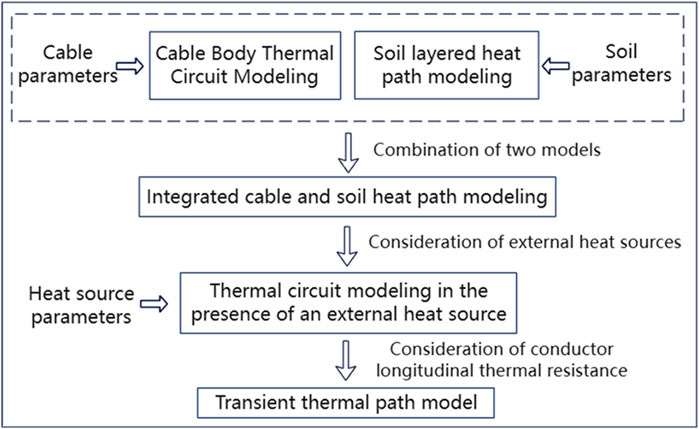
Figure 1. Conceptual framework for thermal circuit model development.

2.2 Transient thermal circuit model of cable body

The transient thermal circuit model utilized for simulating the transverse heat dissipation process of a single-core cable body, as outlined in the IEC 60853 standard, is illustrated in Figure 2 (IEC, 2008). This model incorporates the effects of the heat capacity of each layer on heat dissipation, in contrast to the steady-state thermal circuit model.

Figure 2

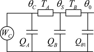
Figure 2. Transient thermal circuit model of a single-core cable body.

Where θ_C is the temperature of the cable core; θ_S denotes the temperature of the outer skin of the cable; θ₀ is the external ambient temperature; and W_C represents both conductor loss and electromagnetic losses of the cable. The equations for the thermal resistance and heat capacity of each layer are presented as follows:

$T_A=T_1(1)$

$T_B=q_s{T}_3(2)$

$Q_A=Q_C+p{Q}_i(3)$

$Q_B=\left(1-p\right)Q_i+\frac{Q_S+p_1{Q}_W}{q_s}(4)$

$Q_{B1}=\frac{\left(1-p_1\right)Q_W}{q_s}(5)$

$p=\frac{1}{2\ln \left(\frac{D_i}{D_c}\right)}-\frac{1}{{\left(\frac{D_i}{D_c}\right)}^2-1}(6)$

$p_1=\frac{1}{2\ln \left(\frac{D_e}{D_s}\right)}-\frac{1}{{\left(\frac{D_e}{D_s}\right)}^2-1}(7)$

$q_s=1+\frac{W_s}{W_c}(8)$

where W_s is the loss of metal sheath and shield; D_c is the outer diameter of the conductor; D_i is the outer diameter of the insulation layer; D_s is the outer diameter of the metal sheath; D_e is the outer diameter of the cable; Q_c, Q_i, Q_s, and Q_w are the heat capacitance of the cable core, the insulation layer, the metal sheath layer, and the outer jacket layer, respectively; while T₁, T₂, T₃, and T₄ are the thermal resistance of the cable’s insulating layer, the inner lining layer, the outer sheath layer, and the external environment, respectively. T₁, T₂, and T₃ are can be determined as follows (YU, 2022):

$T_1=\frac{{\rho }_1}{2\pi }\ln \left(\frac{D_{1o}}{D_{1in}}\right)(9)$

$T_2=\frac{{\rho }_2}{2\pi }\ln \left(\frac{D_{2o}}{D_{2in}}\right)(10)$

$T_3=\frac{{\rho }_3}{2\pi }\ln \left(\frac{D_{3o}}{D_{3in}}\right)(11)$

where ρ₁ is the thermal resistance coefficient of the insulation layer; ρ₂ is the thermal resistance coefficient of the inner lining layer; ρ₃ is the thermal resistance coefficient of the outer sheath layer (K·m/W); while D_o and D_in are the outer and inner diameters of the corresponding layers, mm, respectively.

The external thermal resistance varies depending on the laying conditions. For a single-core power cable that is directly buried in the ground, T₄ is obtained as follows:

$T_4=\frac{{\rho }_T}{2\pi }\ln \left(u+\sqrt{u^2-1}\right)(12)$

where ρ_T is the thermal resistance of the soil (K·m/W) and u is calculated as follows:

$u=\frac{2L}{D_e}(13)$

where L is the distance from the axis of the power cable to the earth surface (mm) and D_e is the outer diameter of the power cable (mm).

Electromagnetic losses consist of eddy current losses and circulating current losses. According to IEC standards, the eddy current loss coefficient is denoted by λ₁′, while the circulating current loss coefficient is represented by λ₁′′. The total loss coefficient (λ₁) is the sum of the two, i.e.:

${\lambda }_1={\lambda }_1^{\prime }+{\lambda }_1^{″}(14)$

The magnitude of electromagnetic losses is given by:

$W_s={\lambda }_{1}W(15)$

where W is the total cable losses, λ1′ is the metallic sheath/armor eddy current loss factor and λ1′′ is the metallic sheath/armor circulating current loss factor.

The hysteresis loss in the cable is negligible due to the use of copper as the conductor material, a non-ferromagnetic metal with relative permeability (μ_r) approximately equal to 1 and a hysteresis loop area approaching zero. For cables containing ferromagnetic materials (e.g., steel armor), hysteresis loss must be modeled separately. Since the 110 kV cable studied in this work features a non-magnetic sheath, this component is excluded. Additionally, the dielectric loss tangent (tanδ) of the cable insulation is ≤0.001. The dielectric loss power density, calculated as W_d = ωCU²tanδ, contributes less than 0.2% to the total losses and is therefore also neglected. Consequently, this study focuses exclusively on conductor losses and electromagnetic losses. By applying Equations 14, 15, both conductor losses and electromagnetic losses are introduced as heat sources into the thermal circuit model, thereby achieving electro-thermal multiphysics coupling.

2.3 Development of multilayer soil thermal circuit model

The multilayer soil model is capable of accurately simulating the diffusion process of heat generated by cables within the soil. Yu (2022) illustrates the applicability of the multilayer soil model through the research and analysis of a five-layer soil thermal circuit model, which facilitates precise calculations of the temperature field associated with a single-core cable. In this layered soil model, each layer is represented by a T-type thermal circuit model, where the thermal resistance of each layer is R and the heat capacity is C. When the soil is stratified into five layers, the corresponding equivalent thermal circuit model is depicted in Figure 3.

Figure 3

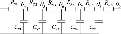
Figure 3. Multilayer soil thermal circuit model for underground cable heat dissipation.

The thermal resistance and heat capacity of each layer are calculated as follows:

$R_m=\frac{{\rho }_T}{2\pi }\log \left(1+\frac{th}{r_{\mathrm{int}}}\right)(16)$

$C_m=\pi \left(r_{ext}^2-r_{\mathrm{int}}^2\right)·C_p(17)$

$R_{s1}=\frac{1}{2}{R}_1(18)$

$R_{si}=\frac{1}{2}\left(R_{i-1}+R_i\right)(19)$

$R_{s6}=\frac{1}{2}{R}_5(20)$

where m is the number of soil layers (m = 1, 2, 3, 4, and 5); th is the thickness of each soil layer; r_ext and r_int are the outer and inner diameters of each soil layer, respectively; C_p is the volumetric specific heat capacity of the soil (J/mm³·°C); and i = 2, 3, 4, and 5.

Soil modeling plays a critical role in assessing the temperature rise effects associated with underground cables. After the dimensions and configuration of the cable have been established, the soil emerges as the primary factor affecting the distribution of the cable’s temperature field. However, the model is predicated on the assumption of a uniform soil environment, which presents certain limitations when confronted with the complexities and variations of the actual operational environment of the cable. Therefore, it is unable to accurately replicate the soil conditions at different locations surrounding the cable.

2.4 Comprehensive cable body and soil thermal circuit model

The integration of the soil-layered thermal circuit model with the thermal circuit model of the IEC standard cable body offers a more comprehensive understanding of the thermal characteristics of the cable. This approach more accurately reflects the complex thermal environment encountered in practical applications, thereby enhancing the reliability and safety of the system while optimizing the design and installation of the cable. This methodology is widely acknowledged due to the continuity in the structure and temperature distribution across each layer of the cable (Qin et al., 2024). The construction of the integrated thermal circuit model is illustrated in Figure 4, where the parameters of the cable body model are developed in accordance with the IEC standard, and the parameters of the soil model are derived from the soil layering model. The integrated thermal circuit model is capable of simulating the heat exchange process between the cable and the surrounding soil environment more comprehensively, thereby providing a more robust theoretical foundation for engineering practice.

Figure 4

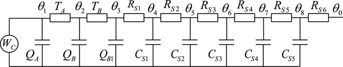
Figure 4. Integrated thermal circuit model combining cable body and multilayer soil.

2.5 Development of thermal circuit model incorporating external heat sources

In practical applications, cables are typically installed in clusters within the soil, and the mutual thermal impacts among these cables affect the temperature distribution in the surrounding environment. When the effects of neighboring cables are incorporated into the thermal circuit model, the temperature field of all underground cables can be efficiently determined using analytical methods, which holds substantial engineering significance (Niu et al., 2023). This study simulates the mutual thermal impact between cables by incorporating the losses from adjacent cables at designated locations within a multilayer soil thermal circuit model. Furthermore, the collective thermal interactions of all neighboring cables are integrated into the RC trapezoidal thermal circuit model of the cables under analysis. Consequently, this approach allows for a more precise modeling of the transient temperature of the cables. The transient thermal circuit model that accounts for the mutual thermal impacts is depicted in Figure 5.

Figure 5

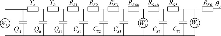
Figure 5. Thermal circuit model incorporating external heat sources.

The losses W_k generated by neighboring cables should be precisely incorporated into their respective locations within the soil model. If an external cable k is situated within the soil thermal resistance (e.g., R_S4), this thermal resistance must be subdivided into two sub-resistances (i.e., R_S4a and R_S4b). The values of these sub-resistances will be allocated proportionally based on the position of the external cable, and a heat source W₁ will be introduced at the junction of the two sub-resistances to ensure the model’s accuracy in calculating the temperature increase of the cable. If the external cable is positioned at a node between two layers of the soil model, it can be effectively simulated by incorporating an additional heat source W₂ into the thermal circuit diagram. Given that the soil thermal circuit model operates on the principle of superposition, it is adequate to add the losses from each cable to the corresponding location in the thermal circuit model that represents the soil. Furthermore, the thermal impacts of other heat sources, such as steam pipes and heating pipes, on the cables can be addressed in a similar manner.

In real-world operating environments, cables are typically affected by a multitude of heat sources. These sources encompass not only the internal heating of the cable and variations in soil temperature but also include surrounding equipment, climatic conditions, and other external factors. This results in a highly complex heat dissipation environment. In contrast, traditional thermal circuit models often operate under the assumption of a simple and uniformly distributed environment, which renders them inadequate for effectively addressing the complexities associated with actual operating conditions.

2.6 Transient thermal circuit modeling considering axial heat dissipation

The temperature of a cable is affected not only by radial heat transfer, which refers to the heat conduction between the conductor and the insulation layer, but also by axial heat flow along the length of the cable. This axial heat flow can create temperature gradients at various locations along the cable. Traditional thermal circuit models frequently overlook the significance of axial heat dissipation when analyzing heat conduction between the conductor and the insulation layer. This oversight can result in inaccuracies in the calculated results and may restrict the model’s precision under certain complex operational conditions.

The schematic diagram of the model, which illustrates the installation of the underground power cable along the center of the street, is presented in Figure 6.

Figure 6

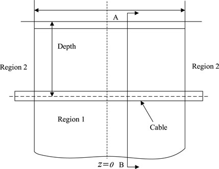
Figure 6. Schematic of cable thermal modeling across a street-crossing segment.

In Figure 6, the area designated for the installation of underground cables is longitudinally divided into two sections. The central portion of the street (Area 1) is characterized as an unfavorable heat dissipation zone with a specified width of b₀. Conversely, the remaining section is Area 2, which represents a standard installation area. Due to the differing soil thermal resistance coefficients in these two areas, a temperature gradient is established along the axial direction of the cable, resulting in the generation of axial heat flow. To analyze the three-dimensional thermal field, the cable is discretized along its length (Z-axis) into N sections, with each segment represented as a small section of the conductor ∆z. The heat flow is illustrated in Figure 7.

Figure 7

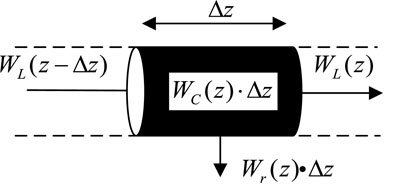
Figure 7. Schematic of heat flow for a discretized section of cable conductor.

Where W_C is the conductor loss generated by the current passed through the cable; W_r is the heat dissipated along the conductor in the radial direction; and W_L is the heat dissipated along the conductor in the axial direction. Due to the different external environmental parameters, there is heat exchange along the cable’s axial direction. Compared with other existing schematic diagrams of heat flow in cable conductor segments, Figure 7 simultaneously considers the influence of radial heat dissipation (W_r) and axial heat dissipation (W_L), achieving a coupled analysis of the cable’s lateral and longitudinal heat conduction. This enables a more accurate simulation of heat exchange in cables under different heat dissipation environments.

According to the law of conservation of energy, the total heat entering a node, combined with the heat generated by the conductor, is equal to the total heat exiting the node. Therefore, the thermal equilibrium equation for the conductor section can be expressed as follows:

$W_C\left(z\right)\Delta z+W_L\left(z-\Delta z\right)=W_r\left(z\right)\Delta z+W_L\left(z\right)(21)$

In comparison to the thermal equilibrium equation of the conventional thermal circuit model, the equation presented in this paper accounts for axial heat dissipation within the cable conductor. The enhanced thermal circuit model is developed using a single-core cable situated in various soil environments as a case study (Figure 8). The neighboring cable segments are connected by axial thermal resistance (T_L) in Figure 8, and each node of each cable segment branch from bottom to top represents the structure of each layer of the cable from the conductor to the soil surface, respectively. This model simultaneously incorporates both radial interlayer conduction and axial intersegment conduction, providing a complete characterization of three-dimensional heat diffusion processes. Given that the heat capacity of the cable conductor is relatively small in comparison to other materials (e.g., insulation and sheath materials), it can be disregarded during the establishment of the thermal circuit model. Furthermore, this model is also applicable to three-core cables, where the transient thermal circuit model is constructed by partially modifying the cable body model to accommodate the three-core configuration (Liu et al., 2016).

Figure 8

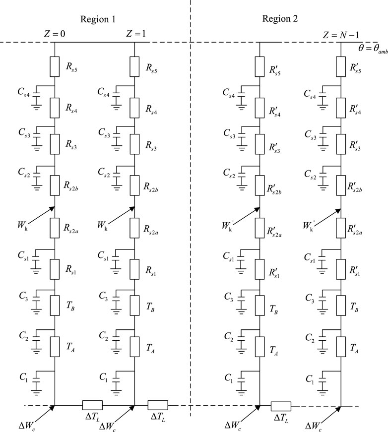
Figure 8. Full-length transient thermal circuit model incorporating axial heat dissipation in heterogeneous environment.

This thermal circuit model delineates the entire area into two regions: unfavorable and normal heat dissipation zones. The coordinate z = 0 is positioned at the center of the unfavorable heat dissipation zone. The axial thermal resistance of the conductor is calculated as follows:

$\Delta T_L=\frac{\rho }{A}(22)$

where ρ is the thermal resistance of the conductor (K·m/W) and A is the cross-sectional area of the conductor (mm³).

W is related to the temperature of the conductor, which can be determined as follows:

$W=W_{20}\left(1+{\alpha }_{20}\left(\theta -20\right)\right)=W_{const}+\delta W·\theta (23)$

$W_{const}=W_{20}\left(1-20{\alpha }_{20}\right)(24)$

$\delta W={\alpha }_{20}{W}_{20}(25)$

where α₂₀ is the conductor’s resistivity temperature coefficient at 20°C, typically valued at 3.93 × 10⁻³ K⁻¹ for copper; and W₂₀ is the conductor loss at the reference temperature:

$W_{20}=I^2{R}_{20}(26)$

where R₂₀ is the AC resistance of the conductor at 20°C, incorporating skin and proximity effects:

$R_{20}=R_{20}^{\prime }\left(1+y_s+y_p\right)(27)$

where R’₂₀ is the DC resistance of the conductor at 20°C. For copper conductors, R^’₂₀ = 1.72 × 10⁻⁸ Ω⋅m; y_s is the skin effect factor, and y_p is the proximity effect factor.

2.7 Transient thermal circuit model solution

The operation of cables involves various metal materials (e.g., conductors, metal sheaths, and armor) along with insulating materials. These components generate losses and emit heat, thereby establishing a heat flow field. The heat flow field exhibits a correspondence with the physical quantities present in both the thermal circuit and the current field. Consequently, it is feasible to employ circuit theory and the principles of the current field to analyze and calculate the thermal circuit model of the cable.

According to the transient thermal circuit model (Figure 8), a thermal balance analysis is conducted for each node. Each node can be represented by a thermal equilibrium equation analogous to Equation 21. In this context, the heat flow between two adjacent nodes is expressed as a function of the temperature difference between the nodes and the thermal resistance. Therefore, Equation 21 can be reformulated as follows:

$C_1\frac{d{\theta }_c\left(n\right)}{dt}+\frac{2{\theta }_c\left(n\right)}{\Delta T_L}-\frac{{\theta }_c\left(n-1\right)}{\Delta T_L}-\frac{{\theta }_c\left(n+1\right)}{\Delta T_L}+\frac{{\theta }_c\left(n\right)}{\Delta T_A}-\frac{2{\theta }_i\left(n\right)}{\Delta T_A}=\Delta W_c\left[n\right](28)$

By expressing thermal resistance in terms of thermal conductance, the complete thermal circuit model can be represented as a system of first-order differential equations following collation:

$C\frac{d\theta }{dt}+Z·\theta =\Delta W(29)$

where θ is the M × 1 temperature matrix to be solved; C is the M × 1 heat capacity matrix; Z is the M × M node conductivity matrix; and ∆W is the M × 1 heat source matrix. In summary, the transient temperature variation at each node of the entire cable can be determined by solving this system of differential equations through thermal node analysis. The procedure for utilizing the thermal node analysis method to assess the temperature rise effect in the cable is depicted in Figure 9.

Figure 9

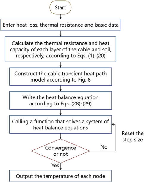
Figure 9. Flowchart of thermal node analysis method for cable temperature modeling.

The parameters of the running cable (e.g., the thermal resistance coefficient and ambient temperature data) are initially incorporated into Equations 1–20 and Equation 22 to determine the thermal resistance and heat loss for each layer within the thermal circuit model. Then, Equations 23–27 are used to compute the heat source magnitude, and these values are subsequently integrated into the transient thermal circuit model of the cable (Figure 8). Finally, the thermal equilibrium equations of the thermal circuit model are derived using Equations 28, 29. The fourth-order Runge-Kutta algorithm is employed to programmatically solve this system of equations, thereby generating the transient temperature rise curve for the entire cable at each node. Finally, the fourth-order Runge-Kutta algorithm is again utilized to program and resolve the equations, yielding the transient temperature rise curve for each individual node of the complete cable system.

3 Validation of transient thermal circuit model

3.1 Experimental verification of transient thermal circuit model’s accuracy

Reference (Zeng et al., 2022) established an experimental system for temperature measurement of a YJLW03 64/110 1 × 500 power cable, with structural parameters detailed in Table 1. The cable was buried at a depth of 800 mm in soil characterized by a thermal resistivity of 1.2 K·m/W and a surface temperature of 20°C.

Table 1

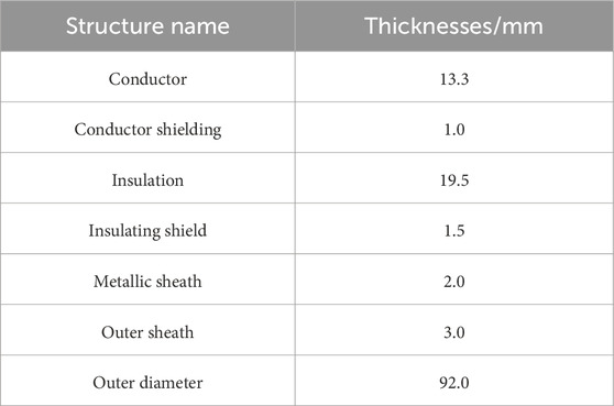
Table 1. YJLW03 64/110 1 × 500 cable structure parameters.

The experimental setup comprised the following components: 380 V power supply, voltage regulator (for input voltage adjustment), PLC control cabinet (for current regulation and data acquisition), computer workstation (for real-time data recording and analysis), current booster (to generate high currents), current transformer (for real-time monitoring of cable load current), compensation capacitor bank (to ensure stability of the test circuit) and the test cable. Thermocouples were employed to measure temperatures across the cable layers. For internal temperature profiling, holes were drilled into the cable body to embed thermocouples within specific structural layers. Surface temperatures were measured by affixing thermocouples directly to the cable exterior. Prior to testing, all thermocouples underwent calibration experiments, and drill holes were sealed with epoxy putty to minimize measurement errors.

To validate the accuracy of the constructed thermal circuit model, a transient thermal circuit model of the experimental cable was established based on the configuration shown in Figure 8. During the modeling process, the soil environment was divided into five equal layers to calculate equivalent thermal resistance and capacitance. Numerical analysis was employed to obtain the hot-spot temperature distribution of the conductor, which was then compared with the experimental results from Reference (Zeng et al., 2022). As shown in Figure 10:

Figure 10

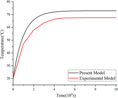
Figure 10. Conductor temperature rise curves obtained by proposed model and experimental method.

Through a comparative analysis utilizing the experimental method, the conductor temperature predicted by this model is marginally higher than the temperature measured experimentally, with a maximum relative error of 7.4%. This discrepancy primarily arises from the thermal circuit model, which is typically constructed based on several simplified assumptions, notably the exclusion of the air gap layer’s effects. This omission results in an overestimation of the thermal resistance value within the model, thereby leading to elevated calculation results. However, the air gap layer does not come into direct contact with the cable conductor, thereby exerting minimal effect on the conductor’s temperature and not compromising the overall accuracy of the results.

3.2 Validation of transient thermal circuit model

To assess the efficacy of the developed thermal circuit model, an analysis was conducted using three single-core YJLW02 64/110 1 × 630 cables as a case study. These cables were arranged horizontally, with their metal sheaths interconnected for grounding purposes. The spacing between the cables was established at 250 mm, and the burial depth was set at 700 mm. It is assumed that the cables traverse a street intersection, leading to the division of the underground cable laying area along the axial direction into two regions. The section of cable located within the street intersection is Region 1, which is characterized by unfavorable heat dissipation conditions. Conversely, Region 2 represents a standard laying environment (Figure 6). The soil thermal resistance coefficients for Regions 1 and 2 are 2.5 K·m/W and 1.0 K·m/W, respectively. The temperature rise effect of the cables was calculated utilizing the thermal circuit model developed in this study, as well as a traditional thermal circuit model and the FEM for comparison. The ambient soil temperature was maintained at 20°C. The structural parameters of the cables are outlined in Table 2.

Table 2

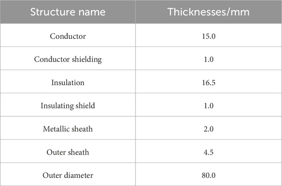
Table 2. YJLW02 64/110 1 × 630 cable structure parameters.

According to national standards, the maximum allowable temperature for the conductor of YJV cable should not exceed 90°C. In the aforementioned calculation example, the cable was initially energized with a 900 A current until reaching steady-state conditions (where the steady-state temperature distribution serves as the initial condition for transient analysis). Subsequently, the current was abruptly increased to 1045 A. A transient thermal circuit model was constructed based on Figure 8, with the cable discretized into 100 segments (0.1 m per segment). Thermal analysis was performed, and the computational results are presented in Figure 11. The model calculates temperatures at all nodes across the 100 segments. For clarity, Figure 11 selectively displays transient temperature rise curves for 10 representative conductor nodes. These curves are arranged in order from top to bottom and correspond to the temperatures of the intermediate conductor nodes that are further and further away from the center of the street (1-m intervals). The horizontal axis represents the elapsed time after the transient current application, while the vertical axis indicates conductor temperature. Transient temperatures for other nodes can be directly extracted from the solution vector θ.

Figure 11

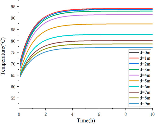
Figure 11. Transient conductor temperature profiles at discrete cable nodes.

In Figure 11, an extended duration of exposure to the step current correlates with an increase in conductor temperature, which stabilizes after approximately 6 h. The steady-state temperature is recorded at 94.1°C, with the highest temperature observed at the center of the street. Furthermore, the conductor temperature exhibits a decreasing trend as the distance from the street center increases. The transient temperature rise curve for this scenario was calculated using both the traditional thermal circuit model and the FEM. A comparative analysis of the temperature change curve at the conductor’s hottest point over time, derived from the three methodologies, is depicted in Figure 12.

Figure 12

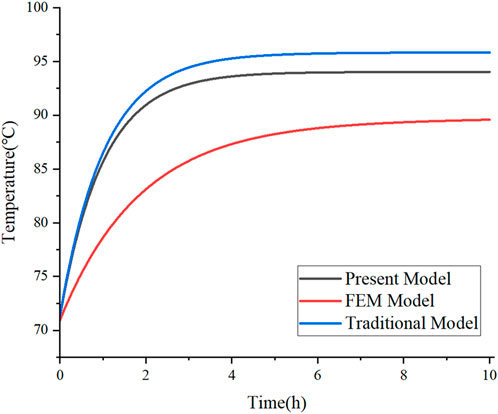
Figure 12. Comparison of conductor temperature rise curves from different methods.

Table 3 summarizes a comparison of the temperature change rule at the hottest point of the conductor over time, as determined by three different calculation methods.

Table 3

Table 3. Comparative results of conductor temperature calculations using three methods.

In Table 3, the calculated temperature derived from the thermal circuit model is higher than that obtained through the FEM. This discrepancy arises from the thermal circuit model’s omission of the air gap layer’s effect during its construction. Using the FEM’s calculation results as a reference point, a comparison is made between the temperature results at the hottest point of the conductor, as determined by both the traditional thermal circuit model and the thermal circuit model developed in this study:the maximum temperature of the conductor, as determined by the thermal circuit model developed in this study, is 94.1°C. This value exhibits a deviation of 4.4°C when compared to the results obtained through the FEM, resulting in a relative error of 4.91%. Furthermore, the maximum discrepancy recorded is 7.2°C, with a corresponding maximum relative error of 8.63%. In comparison to traditional models (Table 3), the error associated with the proposed model is relatively minor, thereby indicating that the computational results are more accurate. Furthermore, while conventional thermal circuit models are limited to simulating and calculating the temporal temperature variations at specific nodes, the thermal circuit model proposed in this paper is capable of assessing the temperature rise effects at any node throughout the entire cable. This capability renders it particularly suitable for a diverse range of cables operating in various heat dissipation environments and multi-heat source scenarios. The comparative analysis of the results from these three methodologies substantiates the efficacy of the constructed thermal circuit model in accurately calculating the transient temperature rise effects of cables, particularly in contexts involving varying heat dissipation conditions.

To further demonstrate the advantages of the proposed model, its computational efficiency, environmental adaptability, and dynamic analysis capabilities are compared with several recent models. Reference (Stojanović et al., 2023) employed the finite element method for multi-field coupling under solar radiation, wind speed, and soil moisture conditions, accurately calculating the transient temperature rise of cables under extreme summer and typical winter conditions. However, compared with our model, the finite element method requires longer computation time and necessitates re-modeling for different cable configurations and installation environments, making it difficult to meet real-time monitoring demands in modern power systems. Reference (Henke and Frei, 2023) proposed a method for determining coupling parameters, which accounts for increasingly complex heat dissipation conditions but is only applicable to parallel-arranged multi-cable scenarios. It introduces errors in non-uniform environmental conditions. In contrast, the thermal circuit model developed in this study can determine the temperature rise at any node along the entire cable, making it suitable for diverse heat dissipation environments and multi-heat-source scenarios. Reference (Ramirez and Anders, 2021) considers the impact of axial heat dissipation on cable temperature, it can only compute steady-state temperature distributions. In real-world operations, cable parameters and environmental conditions are continuously changing. By inputting these dynamic parameters into our thermal circuit model, real-time temperature variations can be calculated efficiently.

4 Conclusion

In light of the increasing complexity of cable laying environments and the challenges in rapidly and accurately predicting cable temperature rise, this paper presents the development of a transient thermal circuit model tailored for power cables. The key results and contributions of this study are summarized as follows:

1) A transient thermal circuit model was developed based on heat transfer theory and the IEC 60853 standard. The model integrates the thermal characteristics of the cable body, a multilayer soil environment, and external heat sources. It incorporates axial thermal resistance within the conductor, making it well-suited for the increasingly complex and non-uniform cable laying environments at present.

2) Leveraging the analogy between thermal and electrical networks, the proposed model was solved using the thermal node analysis method. Validation against experimental data confirms the model’s reliability and computational efficiency.

3) When compared with the FEM, the model exhibited a maximum temperature deviation of 4.4°C at the hottest conductor point, with a relative error of 4.91%. The maximum absolute deviation reached 7.2°C, corresponding to a relative error of 8.63%. Additionally, compared to traditional thermal circuit models, the proposed model provides more precise temperature distribution across the entire cable length under varying heat dissipation environments, highlighting its strong engineering applicability and practical significance.

Data availability statement

The original contributions presented in the study are included in the article/supplementary material, further inquiries can be directed to the corresponding author.

Author contributions

TQ: Validation, Writing – original draft, Conceptualization, Methodology. AM: Resources, Supervision, Writing – review and editing. HS: Software, Writing – review and editing, Validation. XC: Writing – review and editing, Visualization, Validation.

Funding

The author(s) declare that no financial support was received for the research and/or publication of this article.

Conflict of interest

The authors declare that the research was conducted in the absence of any commercial or financial relationships that could be construed as a potential conflict of interest.

Generative AI statement

The authors declare that no Generative AI was used in the creation of this manuscript.

Publisher’s note

All claims expressed in this article are solely those of the authors and do not necessarily represent those of their affiliated organizations, or those of the publisher, the editors and the reviewers. Any product that may be evaluated in this article, or claim that may be made by its manufacturer, is not guaranteed or endorsed by the publisher.

References

Bian, X., Chen, Y., and Zhou, Q. (2023). Dynamic temperature field calculation and short-time allowable ampacity evaluation of submarine cable based on thermal analytical model. High. Volt. Eng. 49 (2), 793–802. doi:10.13336/j.1003-6520.hve.20220667

CrossRef Full Text | Google Scholar

Henke, A., and Frei, S. (2023). Analytical thermal cable model for bundles of identical single wire cables. IEEE Trans. Power Deliv. 38 (5), 3107–3116. doi:10.1109/tpwrd.2023.3272837

CrossRef Full Text | Google Scholar

IEC (2008). Amendment 2 - Calculation of the cyclic and emergency current rating of cables - Part 1: Cyclic rating factor for cables up to and including 18/30 (36) kV. Geneva, Switzerland: International Electrotechnical Commission.

Google Scholar

Lei, F., Chu, J., and Liu, Y. (2023). Fault diagnosis of cable overheating based on semiconductor gas sensing array. Trans. China Electrotech. Soc. 38 (13), 3651–3664.

Google Scholar

Li, C., Shen, P., and Ma, H. (2015). Modeling of soil buried multi-circuit Cables’Temperature field and ampacity calculation. High. Volt. Appar. 51 (10), 63–69. doi:10.13296/j.1001-1609.hva.2015.10.010

CrossRef Full Text | Google Scholar

Li, X., Chen, Y., Liu, J., and Wang, X. (2023). A steady state thermal circuit model analysis of the 10 kV 3-core cable joint considering axial heat dissipation. Power Syst. Clean Energy 39 (10), 56–69.

Google Scholar

Liang, Y. (2016). Technological development in evaluating the temperature and ampacity of power cables. High. Volt. Eng. 42 (4), 1142–1150. doi:10.13336/j.1003-6520.hve.20160405014

CrossRef Full Text | Google Scholar

Liang, Y., and Wang, J. (2022). Transient temperature rise calculation of buried power cable based on thermal circuit model and transient adjoint model. High. Volt. Eng. 48 (9), 3517–3525. doi:10.13336/j.1003-6520.hve.20220142

CrossRef Full Text | Google Scholar

Liu, G., Wang, P., and Li, W. (2016). Calculation model and its verification for cable emergency time of 10kV three-core cable. J. South China Univ. Technol. Nat. Sci. Ed. 44 (2), 81–88. doi:10.3969/j.issn.1000-565X.2016.02.013

CrossRef Full Text | Google Scholar

Liu, G., Wang, P., Zhou, F., and Liu, Y. (2018). Optimization on the insulating layer of transient thermal circuit model of power cable. High. Volt. Eng. 44 (5), 1549–1556. doi:10.13336/j.1003-6520.hve.20180211001

CrossRef Full Text | Google Scholar

Liu, W., Xie, M., and Zhou, Y. (2024). Effects of microstructural parameters of soil on temperature and ampacity of the buried cables. High. Volt. Eng. 50 (2), 749–757.

Google Scholar

Niu, H., Li, X., and Chen, Z. (2023). Phase sequence optimization of tunnel multi-circuit cables based on improved genetic algorithm. Electr. Power Eng. Technol. 42 (2), 147–153.

Google Scholar

Niu, H., Huang, S., and Wang, D. (2025). Digital twin modeling method of temperature field in distribution cables based on reduced order model. J. South China Univ. Technol. Nat. Sci. Ed. 53 (1), 10–20.

Google Scholar

Paweł, O., Piotr, C., and Marcelina, M. (2021). Analysis of an application possibility of geopolymer materials as thermal backfill for underground power cable system. Clean Technol. Environ. Policy 23 (3), 869–878. doi:10.1007/s10098-020-01942-8

CrossRef Full Text | Google Scholar

Qin, X., Zhou, W., and Lv, M. (2024). Inversion of soil thermal conductivity for high voltage power cable. Adv. Technol. Electr. Eng. Energy 43 (9), 94–102.

Google Scholar

Ramirez, L., and Anders, G. (2021). Notice of removal: thermal analysis of multiple cable crossings. IEEE Trans. Power Deliv. 1, 1–8. doi:10.1109/tpwrd.2021.3097953

CrossRef Full Text | Google Scholar

Stojanović, M., Klimenta, J., Panić, M., Klimenta, D., Tasić, D., Milovanović, M., et al. (2023). Thermal aging management of underground power cables in electricity distribution networks: a FEM-based Arrhenius analysis of the hot spot effect. Electr. Eng. 105 (2), 647–662. doi:10.1007/s00202-022-01689-z

CrossRef Full Text | Google Scholar

Tao, X., Zhang, W., and Gong, H. (2023). Research on inversion calculation method of cable temperature based on RFID thermometers. High. Volt. Appar. 59 (4), 116–124.

Google Scholar

Wang, Y., Li, Z., Yang, P., and Liu, W. (2022). Calculation of conductor temperature and ampacity of directly buried cable based on electromagnetic thermal multi field coupling. Acta Metrol. Sin. 43 (7), 877–884.

Google Scholar

Wei, Y., Zhang, J., Li, G., Hu, K., Nie, Y., Li, S., et al. (2023). Material properties and electric thermal stress multiple fields coupling simulation of power distribution CableAccessories. IEEE Trans. Dielectr. Electr. Insulation 30 (1), 359–367. doi:10.1109/tdei.2022.3225694

CrossRef Full Text | Google Scholar

Xu, C., Wang, P., and Yang, F. (2024). Analysis of multi-physics field and temperature gradient field of crimping defects on intermediate joints on the three-core cable. High. Volt. Eng. 50 (4), 1769–1780. doi:10.13336/j.1003-6520.hve.20230812

CrossRef Full Text | Google Scholar

Yu, K. (2022). “Temperature field calculation and dynamic capacity increase of directly buried power cables,” in Master's thesis.Northeast electric power university.

Google Scholar

Zeng, H., Wang, J., and Han, Z. (2022). Transient thermal circuit modeling method for high voltage single core cable based on optimized coating layer. Guangdong Electr. Power 35 (4), 87–95.

Google Scholar

Zhang, A., and He, G. (2023). Real-time prediction of submarine cable embedment depth based on finite element method. J. Electron. Meas. Instrum. 37 (12), 18–28.

Google Scholar

Zhang, H., Zhou, H., and Ye, Z. (2021). Analytical calculation and experiment research on real-time ConductorTenmerature of three-core cable. Electr. Eng. 17, 1–4. doi:10.19768/j.cnki.dgjs.2021.17.001

CrossRef Full Text | Google Scholar