Real defect partial discharge identification method for power cables joints based on integrated PJS-M and GA-SVM algorithm with multi-source fusion

Previous studies on 10 kV cable intermediate joint defects have mainly focused on typical defect types and employed single-sensor data acquisition, leading to incomplete characterization of defect features and reduced recognition accuracy. To address this limitation, three real-type partial discharge (PD) models were developed based on common defects encountered in actual manufacturing. PD signals were collected using a combination of High-Frequency Current Transformer (HFCT) and Ultra High Frequency (UHF) sensors, capturing time-domain waveforms, frequency-domain spectra, and Phase-Resolved Partial Discharge (PRPD) patterns, from which feature quantities were extracted. These features were used to train a novel Genetic Algorithm Weighted Support Vector Machine (GAW-SVM) model, which incorporates an adaptive PJS-M weighting coefficient and a correlation-analysis–based dynamic correction mechanism into the conventional GA-SVM framework. The proposed model was compared with several state-of-the-art SVM optimization algorithms, including GA-SVM, PCA-SVM, and PSO-SVM. Under multi-source feature fusion, the GAW-SVM achieved a defect recognition accuracy of 98.84%, outperforming GA-SVM by 3.49%, PCA-SVM by 2.33%, and PSO-SVM by 1.17%. These results demonstrate that the proposed method significantly improves the accuracy of identifying complex real-type defects in 10 kV cable intermediate joints under multi-source feature conditions, providing a reliable diagnostic basis and technical reference for partial discharge detection in industrial applications.

1 Introduction

With the accelerating pace of urbanization and rural revitalization in China, the installation of 10 kV XLPE cables in the power grid has been increasing annually. Therefore, the online monitoring of cable operating conditions has become particularly important to ensure that preventive measures are taken before faults occur. Cable intermediate joints, as weak links in power cables, are susceptible to defects caused by factors such as manufacturing processes and installation quality, including issues such as the tips of the outer semi-conductive layer, scratches or cuts in the main insulation, and misalignment of the stress cone during installation. During long-term operation, these defects can lead to various types of partial discharges, such as corona, surface, floating, and air-gap discharges, under the influence of high voltages and environmental factors. These discharges seriously threaten the insulation performance of cables and shorten their service lives (Wojciech and Artur, 2023). Therefore, monitoring the early stage phenomena of partial discharge, classifying the discharge types, and determining the defect discharge types in a timely manner are essential to reduce their effect on the power grid (Cavallini et al., 2005).

Different defects in cable joints generate different electric field distributions under high voltages, and engineering practices distinguish defect types based on the differences in the discharge spectra (Yuanhu et al., 2023). Through partial discharge monitoring, defect types can be identified, with the process mainly involving feature extraction and classification, where feature extraction is crucial for recognition task (Liu et al., 2022; Rosta et al., 2016). Currently, scholars mainly use one or two features, such as the discharge pulse time-domain, frequency-domain, and phase-distribution features, to extract the feature quantities for typical defects (Shang et al., 2017; Bo et al., 2022; Korobeynikov et al., 2019). Jing-Hai Jiao extracted discharge timing waveforms, transforming the one-dimensional partial discharge signal into a two-dimensional topological feature image through feature transformation, and incorporated an attention mechanism into the Residual Network ResNet101 model, combining Center and Softmax loss functions for training and classification (Jiao and Jie, 2023). Jing Wu used wavelet theory, wavelet energy spectrum theory, and phase modulation transformation theory to extract and analyze the time-frequency combined features of defects and proposed a fault recognition algorithm based on wavelet energy spectrum of modulated components (Wu, 2014). Yekun Men extracted and analyzed harmonic feature patterns based on the grounding current signal of cables under typical defect types using a fast Fourier transform with a Blackman window and combined it with a backpropagation neural network to achieve effective fault identification of distribution cables (Yekun et al., 2024). Mei Yang extracted multiple types of fractal features from the gray matrix of defect feature maps as recognition feature quantities, with local discharge pattern recognition chosen to use a back propagation neural network (BPNN) (Yang, 2006).

In summary, current research by both domestic and international scholars has primarily focused on single-sensor analysis based on typical defect models (Chang et al., 2022; Sitong et al., 2018). However, compared with typical defect models commonly used under laboratory conditions, real-type defects more accurately reflect the complex and variable conditions encountered in actual operating environments. Therefore, diagnostic criteria derived solely from typical defects often fail to represent the true state of engineering systems. Moreover, most existing studies still concentrate on the extraction and analysis of single-domain features—such as time-domain, frequency-domain, or phase-domain features. These single-domain features carry limited information when dealing with complex discharge signals, resulting in significantly reduced recognition accuracy and making them inadequate for precise fault diagnosis. Finally, the widely adopted conventional algorithm was not originally designed to handle the fusion and processing of multi-source, heterogeneous features. It lacks the representational capacity needed for high-dimensional joint features, making it difficult to fully exploit the correlations among multi-domain and multi-scale information. Consequently, it cannot provide a reliable and effective basis for practical engineering applications. To address the above issues, this study proposes an improved GA-SVM algorithm based on the PJS-M method, enabling accurate identification of complex real-type defects through the fusion of multi-source feature sets.

Based on this, and building upon previously established typical defect models, this study constructed three real defect cable samples by referencing actual engineering conditions. These samples simulate three types of real defects commonly encountered during the fabrication of cable intermediate joints. Partial discharge (PD) data from the same defect cable were collected using different sensors. A total of 31-dimensional features were extracted, including statistical features of time-domain waveforms, statistical features of frequency-domain spectra, and PRPD pattern features such as statistical characteristics, gray-level moment features, and gray-level texture features. The fused features were then classified using a GAW-SVM algorithm improved by the PJS-M weighting coefficient and correlation analysis, providing a practical method and reference basis for the industrial application of partial discharge detection.

2 Real-type partial discharge testing system for power cable joints

2.1 Selection of real-type defects in cable intermediate joints

Based on a comprehensive analysis of industry failure statistics, international standard provisions, and partial discharge mechanisms, this study ultimately selects three representative real-type defects: outer semiconductive layer tip defects, main insulation scratch defects, and stress cone misalignment defects. According to the CIGRE WG B1.57, 2023 service survey, approximately 80% of cable breakdowns originate from installation defects at joints or terminations. Supporting this, experimental data collected in this study show that these three defect types account for roughly 70% of early failure cases in cable joints.

International standards provide explicit risk descriptions regarding residual sharp tips, insulation scratch depth, and stress cone misalignment, reflecting the strict engineering control requirements associated with these defects. From a discharge mechanism perspective, the three selected defects correspond to surface-type, volume-type, and interface-type partial discharges, respectively, forming a minimally complete set of failure mechanisms. This also enables comprehensive validation of the applicability of the proposed multi-source fusion diagnostic algorithm.

Therefore, focusing on these three defect types not only ensures high representativeness but also significantly enhances the practical value of the proposed method in real-time condition assessment and maintenance decision-making for cable systems.

2.2 Real-type defect setup for cable intermediate joints

Based on the defect types selected in the preceding section, three real-type defect configurations were implemented on 10 kV XLPE cable intermediate joints using a real-condition experimental platform. The defect fabrication process simulates the actual procedures and conditions encountered during cable installation in power systems, ensuring that the defects closely resemble those found in industrial applications. The setup is illustrated in Figure 1. A 4-m-long defect-free cable was divided into two 2-m segments, which were connected using a CSS-1733J-8.7/15 kV cold-shrink joint. The test cable model was ZH-YJV with a cross-sectional area of 185 mm² and a rated voltage of 8.7/15 kV.

1) Construction of outer semi-conductive layer-tip defect: During the production of intermediate cable joints, the semi-conductive layer is usually beveled using a wallpaper knife. However, if not handled carefully, sharp burrs can form at the beveled edges of the outer semi-conductive layer. This defect model was designed to simulate the discharges caused by the concentration of electric field forces at the internal composite insulation interface of the cable joint. To make the partial-discharge signal more stable and easier to detect, the length of the semi-conductive tip was designed to be 25 mm with a width of 10 mm. After inserting the stress cone, the tip defect protruded 5 mm from the semi-conductive part of the stress cone, disrupting the balanced electric field near the tip because of the presence of a sharp edge.

2) Construction of main-insulation scratch defect: During the construction of cable joints, improper handling of the outer semi-conductive layer can damage the main insulation, potentially leading to a partial discharge. The defect model was created by scratching along the axis of the main-insulation surface using a wallpaper knife. The scratch was approximately 20 mm long, 1 mm wide, and 2 mm deep. This defect primarily simulates the discharge-type that occurs when air gaps or voids are formed in the main insulation.

3) Construction of stress cone misalignment defect: During installation of the cold-shrink intermediate joint, the tail of the stress cone should maintain a stable electrical connection with the outer semi-conductive layer of the cable. If the installation is not precise and results in a misalignment such that the outer semi-conductive layer is misaligned with or even extends beyond the stress-cone tail, the stress cone can float above the main-insulation layer, causing floating discharge. When the voltage is significantly high, the outer semi-conductive layer can cause a surface discharge along the main-insulation axis. This defect can extend the misalignment distance of the stress cone by 15 mm. The stress-cone misalignment defect model was used to generate a floating discharge or surface discharge caused by the electric field concentration from the misalignment between the stress cone and the break in the outer semi-conductive layer.

Figure 1

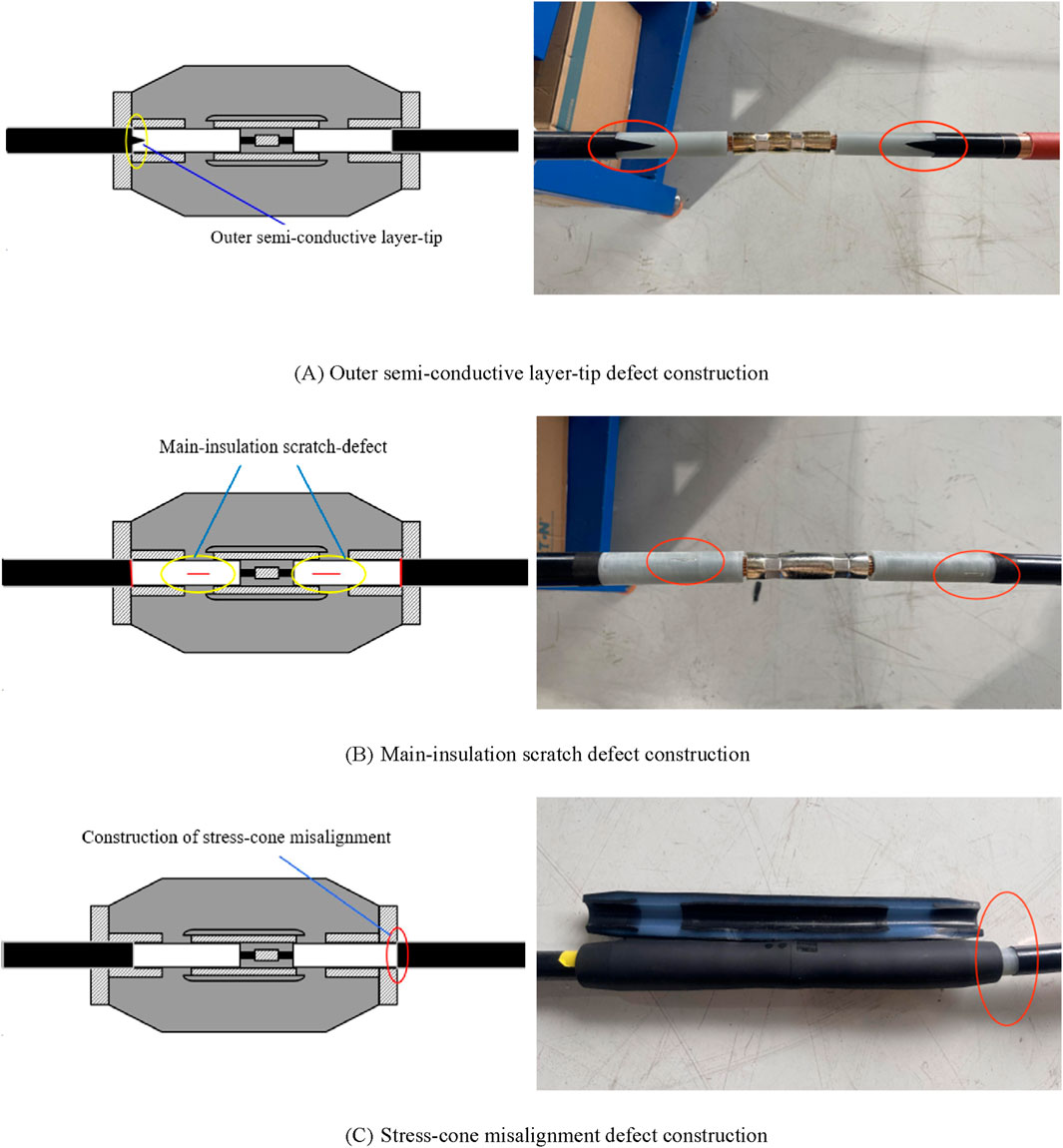
Figure 1. (A) Outer semi-conductive layer-tip defect construction (B) Main-insulation scratch defect construction (C) Stress-cone misalignment defect construction. Structural diagram and photographs of actual defects in cable joints.

To minimize the suppression and interference from the discharge defect signals, none of the three defects were coated with silicone grease during fabrication, and no copper mesh was applied during joint construction. The two cable segments were grounded using a grounding strap connected to the outside of the joint.

2.3 Design and construction of a real experimental platform

A real experimental platform for power cables is shown in Figure 2 and comprises three parts: a power supply system, real cable system, and discharge signal measurement system. The power supply system comprised a signal generator and a co-phase high-voltage amplification coupling power supply. The cable system comprised defect-free cables, artificially defective cable joints, and other accessories. The discharge signal measurement system was designed to use multiple types of sensors for a more comprehensive fusion data analysis of defects. Therefore, two signal measurement systems were designed to measure different types of signals. However, the signal collection of both systems was synchronized to ensure data consistency. Meanwhile, to ensure cost-effectiveness and the feasibility of measurement, all equipment used in the experiments consists of commonly employed devices in practical engineering applications.

1) The discharge signal’s time-domain and frequency-domain waveform data were collected via a high-frequency current transformer (HFCT) using a digital storage oscilloscope (DSO). The frequency range of the HFCT sensor was 10 kHz–100 MHz. The DSO is a Tektronix MDO3014 with four channels, maximum sampling rate of 5 G/s, and record length of 10 M. In this study, sampling channel two was selected, with a sampling rate of 5 G/s and a record length of 10 M. During the measurement, the HFCT sensor was clamped to a cable-shield ground wire.

2) The PRPD spectrum of the discharge signal was collected and displayed on a partial discharge (PD) detector using an ultra-high-frequency (UHF) sensor. The sampling bandwidth of the UHF sensor ranged from 300 MHz to 1,500 MHz. The sensor operates at a sampling frequency of 5 GHz to satisfy the Nyquist sampling criterion. The handheld partial discharge detector was an EPD-800A model. To reduce the shielding effect of the intermediate joint on the UHF signals, the UHF sensor was placed at the end of the joint during measurement.

Figure 2

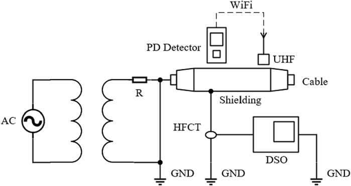
Figure 2. True-scale experimental platform for power cables.

2.4 Pressurization and sampling method

To accurately reflect the discharge patterns, reduce the sampling data volume, and avoid interference from the randomness of the discharges, the partial discharge starting voltage and stable discharge voltage were first determined using a pulse current method partial discharge detector. The measurement system is shown in Figure 3.

Figure 3

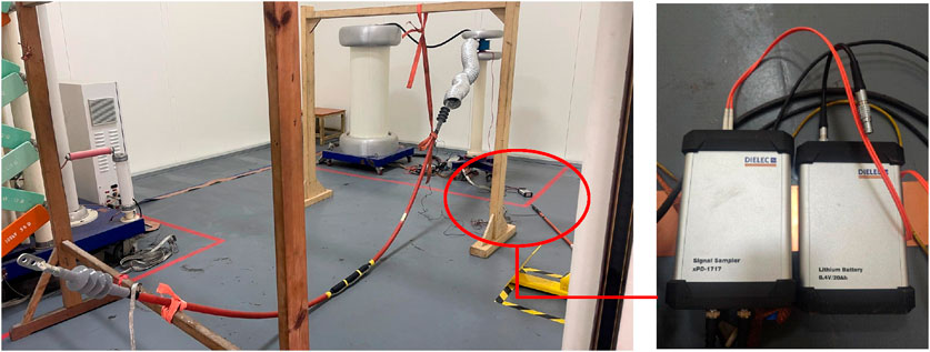
Figure 3. Starting voltage measurement platform.

The pulse current method partial discharge instrument used was the xPD-1717 model with a working voltage of DC 8.4 V. When the partial discharge signals first appeared on the PC, the discharge-starting voltage U₀ was recorded. When the discharge became more evident and the discharge signal stabilized, a stable discharge voltage U_m was recorded, as detailed in Table 1.

Table 1

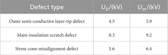
Table 1. Partial discharge voltages of cable-defect models.

To ensure that the three jointed cable samples were subjected to identical voltage stress conditions and to induce sufficiently clear and representative defect discharges, a unified voltage application scheme—comprising synchronous ramp-up, voltage hold, and ramp-down phases—was employed in this study. The voltage was gradually increased from zero to 10 kV, during which discharge signals were monitored. Once stable discharge behavior was observed, both HFCT and UHF sensors were used to perform continuous sampling over equal time durations.

As a result, 217 sets of partial discharge (PD) data were obtained for the outer semi-conductive tip defect, 230 sets for the main insulation scratch defect, and 223 sets for the stress cone misalignment defect. In terms of PRPD patterns, 141 were acquired for the outer semi-conductive tip defect, 132 for the insulation scratch defect, and 157 for the stress cone misalignment defect.

Considering that the dataset exhibits a near-balanced distribution—sufficient to ensure classifier performance is not adversely affected—and to avoid irreversible damage to test samples due to over-pressurization, no effort was made to forcibly equalize the number of samples across defect types.

3 Experimental results and analysis

3.1 Principle and procedure of wavelet transform filtering

The fundamental concept of wavelet transform is to decompose a signal using wavelet basis functions, which are combinations of a series of low-pass and high-pass filters, to capture different frequency components through scaling and translation. The scale parameter controls the width of the wavelet, while the translation parameter determines its position, thereby effectively separating the noise components from the signal. Subsequently, noise suppression is performed on the decomposed coefficients, and the signal is reconstructed to achieve the purpose of denoising. The specific implementation steps are as follows:

1) Selection of the wavelet basis function: An appropriate wavelet basis function is chosen based on the characteristics of the signal, such as Daubechies wavelets, Haar wavelets, Symlet wavelets, or Morlet wavelets.

2) Wavelet decomposition: The signal is decomposed into different scales using the discrete wavelet transform (DWT) through multiresolution analysis, yielding approximation coefficients (A_C), which represent the low-pass filtered components, and detail coefficients (D_C), which represent the high-pass filtered components. The decomposition process typically employs downsampling to reduce the signal length and computational complexity. The same procedure is repeatedly applied to the approximation coefficients for multilevel decomposition. For a discrete signal x [n], the DWT decomposes it into approximation coefficients. Where: φ_j,n is the scaling function, which is used for reconstructing the approximation coefficients, and ψ_j,n is the wavelet function, which is used for reconstructing the detail coefficients. The approximation coefficients A_C is given by Equation 1. The detail coefficients D_C is given by Equation 2.

$A_{Cj}={\displaystyle \sum _n}x\left[n\right]·{\phi }_{j,n}(1)$

$D_{Cj}={\displaystyle \sum _n}x\left[n\right]·{\psi }_{j,n}(2)$

3) Thresholding: A threshold value is determined based on the noise level, and the detail coefficients are processed using either hard thresholding (HD) or soft thresholding (ST). Assuming the threshold is λ, the hard thresholding is given by Equation 3, and the soft thresholding is given by Equation 4. Where: sign denotes the sign of the signal amplitude.

${\widehat{D}}_{Cj}=\left\{\begin{array}{l}{D}_{Cj},\left|D_{Cj}\right|\ge \lambda \\ 0,\left|D_{Cj}\right|<\lambda \end{array}\right.(3)$

${\widehat{D}}_{Cj}=\left\{\begin{array}{l}sign\left(D_{Cj}\right)·\left(\left|D_{Cj}\right|-\lambda \right),\left.D_{Cj}\right|\ge \lambda \\ 0,\left|D_{Cj}\right|<\lambda \end{array}\right.(4)$

4) Wavelet reconstruction: The denoised signal is reconstructed from the processed coefficients using the inverse discrete wavelet transform (IDWT). Reconstruction at each level involves upsampling and filtering operations. The denoised signal is given by Equation 5.

$\widehat{x}\left[n\right]={\displaystyle \sum _j}\left({\widehat{A}}_{Cj}·{\phi }_{j,n}+{\widehat{D}}_{Cj}·{\psi }_{j,n}\right)(5)$

The above equations are used to implement the filtering and denoising of defect discharge signals in both the time and frequency domains.

3.2 Time-domain signal spectrum analysis

Figure 4 shows the time-domain waveforms collected using an HFCT sensor under a 10 kV voltage level for the three types of real defects after noise filtering.

Figure 4

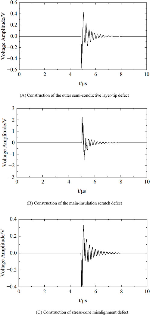
Figure 4. (A) Construction of the outer semi-conductive layer-tip defect (B) Construction of the main-insulation scratch defect (C) Construction of stress-cone misalignment defect. Time-domain spectrum of cable defect discharge.

From the figure, the following can be observed:

1) The discharge amplitude of the outer semi-conductive layer-tip defect was relatively low, with the maximum positive discharge amplitude of approximately 400 mV and the maximum negative discharge amplitude of approximately 580 mV. The discharge shows asymmetry between the positive and negative half-axes, with a noticeable discharge concentration and clear height of the discharge clusters.

2) The discharge amplitude of the stress-cone misalignment defect was the lowest, with the positive and negative half-axes exhibiting asymmetry. The maximum positive discharge amplitude is approximately 320 mV, and the maximum negative discharge amplitudes were approximately 400 mV. After discharge, the amplitude exhibited non-uniform attenuation.

3) The discharge amplitude of the main-insulation scratch defect was relatively high, and the positive and negative half-axes exhibited asymmetries. The maximum positive discharge amplitude was approximately 2.4 V, and the maximum negative discharge amplitude was approximately 1.5 V. After discharging, the amplitude decayed quickly.

3.3 Frequency-domain signal spectrum analysis

Figure 5 shows the frequency-domain spectra of the three types of real defects collected using an HFCT sensor under a 10 kV voltage level after noise filtering.

Figure 5

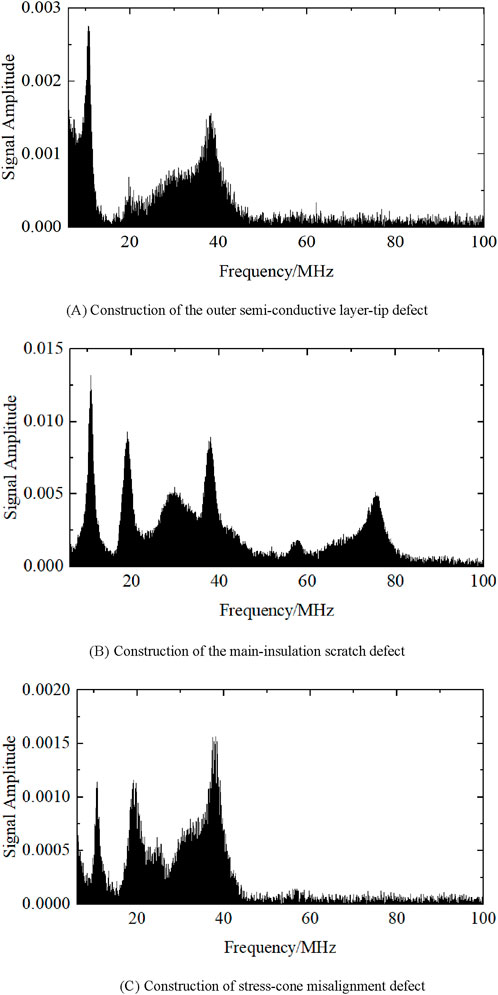
Figure 5. (A) Construction of the outer semi-conductive layer-tip defect (B) Construction of the main-insulation scratch defect (C) Construction of stress-cone misalignment defect. Frequency-domain spectrum of cable defect discharge.

Evidently, both the outer semi-conductive layer-tip defect and the stress-cone misalignment defect exhibit a relatively narrow frequency domain bandwidth concentrated between seven and 45 MHz. However, the spectrum of the outer semi-conductive layer-tip defect has a bimodal shape, whereas the spectrum of the stress-cone misalignment defect has more denser peaks. Therefore, the peak density of the stress-cone misalignment defect is higher than that of the outer semi-conductive layer-tip defect; however, the outer semi-conductive layer-tip defect has higher amplitude in the spectrum. The spectrum amplitude of the main-insulation scratch defect was significantly higher than those of the other two defects, with the highest peak at 0.013. Its frequency-domain bandwidth was broader, with a maximum bandwidth of 75 MHz.

From the spectrum, it is also possible to understand that the total harmonic distortion of the different defects varies considerably.

3.4 PRPD spectrum analysis

As shown in Figure 6, the PRPD patterns of the three types of actual defects at the 10 kV voltage level were collected using the UHF sensor. In the figure, the colors red, yellow, and green represent different ranges of discharge repetition counts: green indicates a discharge count between 0 and 20, yellow represents a count between 20 and 40, and red corresponds to a count greater than 40.

Figure 6

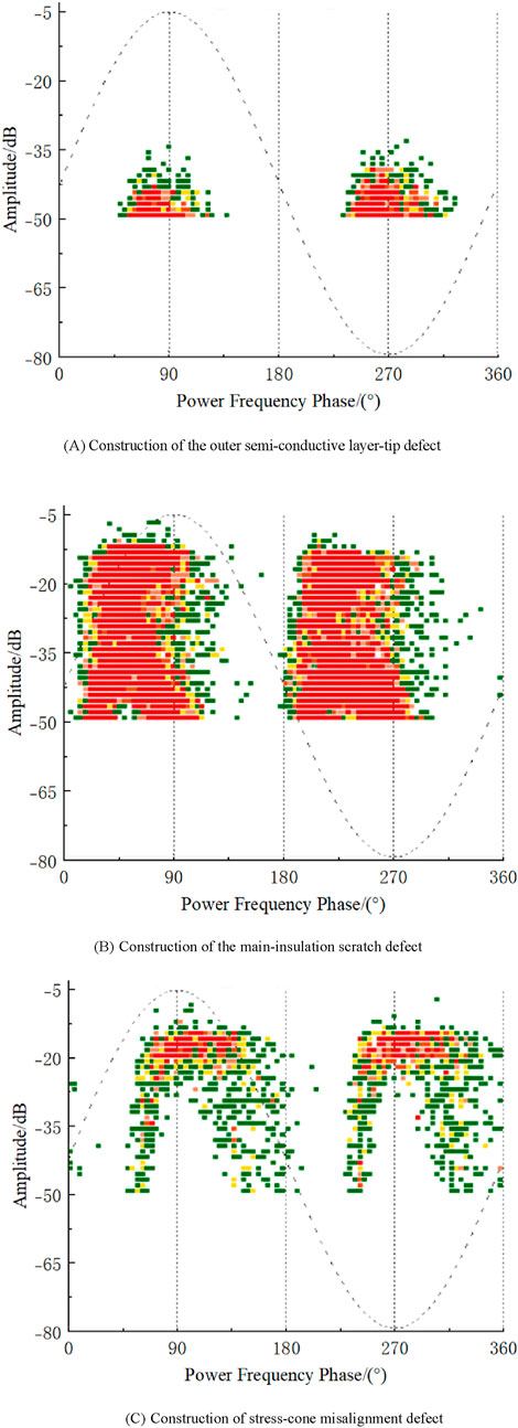
Figure 6. (A) Construction of the outer semi-conductive layer-tip defect (B) Construction of the main-insulation scratch defect (C) Construction of stress-cone misalignment defect. PRPD spectrum of cable defect discharge.

Evidently, the PRPD spectra of the three types of defects exhibit several differences: the discharge points of the outer semi-conductive layer-tip defect are mainly concentrated in the power frequency phase ranges of 50°–120° and 230°–310°. The amplitude distribution of the positive and negative half-cycles of the power frequency shows significant differences, with the positive half-cycle amplitude range between −50 and −40 dB, and the negative half-cycle amplitude range between −50 and −33 dB. The discharge amplitudes near 90° and 270° are higher, with a higher concentration of discharges at lower amplitudes. The overall shape of the spectrum was triangular, with a general leftward shift in the profile. The discharge signals of the main-insulation scratch defects were present in the power frequency phase ranges of 0°–170° and 180°–350° and were mainly distributed between 0°–90° and 180°–270°. The distribution patterns of the positive and negative half-cycles are generally similar; however, the discharge amplitude in the positive half-cycle is slightly higher (approximately 5 dB) than that in the negative half-cycle. The overall shape of the spectrum was trapezoidal, with a leftward shift indicating more intense discharges, and the discharge points were densely distributed across the entire amplitude range. The discharge range of the stress-cone misalignment defect was between the power frequency phases of 60°–200° and 240°–360°, with most of the discharge points concentrated in the second and fourth quadrants. The differences in the contours and distribution of the discharge patterns in the positive and negative half cycles are small. The discharge amplitude is higher and concentrated between −25 and −15 dB, and the distribution of discharge signals roughly forms a “gate” shape.

From the contour features of the PRPD patterns, it is visually evident that there are significant differences between real defects and typical defects. Under more complex actual operating conditions in practical production, it is necessary to investigate defect identification methods tailored to complex discharge patterns, in order to enhance the practical relevance of the results for actual operating conditions.

3.5 Summary of experimental results and analysis

Based on the above analysis, it can be concluded that the time-domain waveforms, frequency-domain spectra, and PRPD spectra of the different defects have varying degrees of distinguishable features. For spectra with obvious characteristics, the defect type can be identified through a relatively straightforward visual differentiation. However, for spectra that are more difficult to distinguish, feature extraction and algorithms are necessary.

4 Feature extraction

4.1 Time-domain signal feature extraction

Based on the analysis of the time-series signal in the previous section, the following features were extracted according to the waveform characteristics: The specific meanings and expressions are as follows.

Signal energy: Describes the total power or energy of the signal, representing the magnitude of the signal’s energy. where y(t) is the time-domain signal amplitude, T is the discharge signal period, and E_c is given by Equation 6.

$E_c={\displaystyle \sum _{t=0}^T}{\left|y\left(t\right)\right|}^2(6)$

Crest Factor: The ratio of the peak value to the root mean square (RMS) value of the signal, characterizing the relative strength of the spikes to the average energy and the instantaneous peak characteristics in the time-domain signal. The CrestFactor is given by Equation 7.

$CrestFactor=\mathit{max}\left(\left|y\left(t\right)\right|\right)\sqrt{\frac{1}{T}{\displaystyle \sum _{t=0}^{T-1}}{\left|y\left(t\right)\right|}^2}(7)$

Kurtosis describes the sharpness or concentration of a signal waveform. A waveform with a higher kurtosis indicates sharper peaks, whereas a waveform with a lower kurtosis indicates a flatter signal. Where: E is the mathematical expectation, x is the sample amplitude of the signal, and μ is the mean value of the signal. The Kurtosis is expressed using Equation 8.

$Kurtosis=\frac{E\left[{\left(x-\mu \right)}^4\right]}{{\left(E\left[{\left(x-\mu \right)}^2\right]\right)}^2}(8)$

Attenuation coefficient: The ratio of the average amplitude of the signal during the initial discharge period to the average amplitude after signal attenuation. The attenuation coefficient A_c of the signal can be expressed using Equation 9, where M₁ is a segment of the fault time during the initial discharge, and M₂ is a segment of time after the signal is attenuated.

$A_c=\frac{1}{M_1}{\displaystyle \sum _{i=1}^{M_1}}\left|y_i\left(t\right)\right|/\frac{1}{M_2}{\displaystyle \sum _{j=1}^{M_2}}\left|y_j\left(t\right)\right|(9)$

Based on these feature parameters, a four-dimensional time-domain feature vector set was obtained.

4.2 Frequency-domain signal feature extraction

From the frequency spectrum, it can be observed that the frequency spectrum amplitude, bandwidth, and frequency distribution differ for various types of defects in real defective cables. Based on these characteristics, the frequency-domain signal features were extracted using the following calculations:

Frequency amplitude ratio: the ratio between the amplitudes of different frequency bands within a certain frequency range. Where N₁ and N₂ are the sample numbers in the first and second frequency bands, respectively. P(k) and P(f) represent the signal amplitudes in the first and second frequency bands, respectively. The frequency amplitude ratio F_ar is given by Equation 10.

$F_{ar}=\frac{1}{N_1}{\displaystyle \sum _{i=1}^{N_1}}{P}_i\left(k\right)/\frac{1}{N_2}{\displaystyle \sum _{j=1}^{N_2}}{P}_j\left(f\right)(10)$

The total Harmonic Distortion: Reflects the ratio of harmonic components to the fundamental frequency component. Where: N is the number of harmonics, and k₁ is the fundamental frequency. The total harmonic distortion T_hd is given by Equation 11.

$T_{hd}=\frac{1}{N}\sqrt{{\displaystyle \sum _{n=2}^N}{\left|y\left(n{k}_1\right)\right|}^2}/y\left(k_1\right)(11)$

Spectral peak density: The ratio of the number of spectral peaks exceeding the mean value within a certain frequency range to the total number of spectral peaks in that range, which describes the complexity of the spectrum. where M is the number of spectra within the frequency range, P(h) is the amplitude of the signal in the frequency band, P_a(h) is the average amplitude of the frequency band. The spectral peak density S_pd is given by Equation 12.

$S_{pd}=\left({\displaystyle \sum _{i=1}^M}\left|P_i\left(h\right)\right|>P_a\left(h\right)\right)/M(12)$

Based on these feature parameters, a three-dimensional frequency-domain feature vector set is obtained.

4.3 PRPD spectrum feature extraction

4.3.1 Statistical parameters features

Statistical features primarily describe the two-dimensional spectrum. The profile differences of the spectra were described by calculating the skewness (SK) and kurtosis (Ku) of the positive and negative half-cycle spectra of the spectrum are described (Deb et al., 2002). The total discharge amount, Q₀, was calculated by the superposition of the discharge amplitudes and counts to represent the energy differences in the spectrum. Finally, a three-dimensional PRPD spectrum statistical feature vector set was extracted.

4.3.2 Gy-level moment parameters features

Gray-level processing is an important technique in computer vision for analyzing image features because it simplifies data, enhances features, and improves processing efficiency (Chen et al., 2022). The PRPD spectrum of the three types of real defects in the cables were converted into grayscale images, and the corresponding grayscale images were generated. The interval was divided into the phase × discharge amplitude (362 × 395). A grayscale value of 0 represents the highest discharge frequency and a grayscale value of 255 represents no discharge. This transformed the grayscale value into a matrix with numerical values ranging from 0 to 255. The grayscale value of each grid was calculated using Equation 13, where RGB_a,b is the grayscale value at coordinates (a, b) in the image, c_a,b is the numerical value of the grid, and c_max is the maximum value among all grids.

$RG{B}_{a,b}=\left(1-c_{a,b}/c_{\max }\right)\times 255(13)$

Moment features describe characteristics such as shape, orientation, and size of the image. Various moment features have been proposed for image analysis (Hu, 1962), in which the central moment, central distance, and second-order central moments were chosen as the main research parameters. For the grayscale image f(x, y), the p + qth order moment is given by Equation 14.

$m_{pq}={\displaystyle \sum _x}{\displaystyle \sum _y}{x}^p{y}^{p}f\left(x,y\right)(14)$

When p = 0 and q = 0, m₀₀ represents the sum of all the grayscale values in the image. The centroid of the grayscale image (x₀, y₀) is the ratio of the first-order moment to the zero-order moment and is calculated using Equation 15.

$\left\{\begin{array}{ll}{x}_0=\frac{m_{10}}{m_{00}}& \\ & \\ y_0=\frac{m_{01}}{m_{00}}& \end{array}\right.(15)$

The p + qth order central moment of the grayscale image f(x, y) is given by Equation 16.

$u_{pq}={\displaystyle \sum _x}{\displaystyle \sum _y}{\left(x-x_0\right)}^p{\left(y-y_0\right)}^{q}f\left(x,y\right)(16)$

The second-order central moments are represented by inertia parameters u₀₂ and u₂₀. Here, u₀₂ represents the moment in the horizontal direction, and u₂₀ represents the moment in the vertical direction. The grayscale image is more widely distributed in the direction of the larger moment and vice versa. The principal axis direction feature is the ratio of these two second-order central moments, which describes the shape features of the grayscale image, and is calculated using Equation 17.

$v=\frac{u_{20}}{u_{02}}=\frac{m_{20}{m}_{00}-m_{10}^2}{m_{02}{m}_{00}-m_{01}^2}(17)$

From Equations 10–12, a five-dimensional moment parameter feature vector set is extracted from the PRPD spectrum.

4.3.3 Gy-level texture parameters features

Gray-level texture features primarily describe the distribution and variation of grayscale values in local regions of an image, providing information about the arrangement of grayscale values in the image. The gray-level co-occurrence matrix (GLCM) method, proposed by Professor Haralick R M, is one of the most fundamental methods for texture feature extraction (Haralick et al., 1973). The GLCM provides comprehensive information regarding the gray-level distribution of the image based on the direction, adjacent intervals, and change amplitude.

In this study, four linearly uncorrelated features were selected based on the literature, and their meanings and expressions are as follows:

Angular second moment (ASM) describes the uniformity of the grayscale distribution. A smaller energy value indicates a more uneven distribution and vice versa. The formula is as shown in Equation 18:

$ASM={\displaystyle \sum _{e=0}^{K-1}}{\displaystyle \sum _{l=0}^{K-1}}{P}_{t,\alpha }{\left(i,j\right)}^2(18)$

where (e, l) represents the element coordinates in the co-occurrence matrix, t is the distance between two pixel points, α is the angle between the two and the horizontal axis, K is the grayscale level, and P_t,α(i,j) is the element value at coordinate (i, j) in the co-occurrence matrix.

Entropy (ENT) reflects the richness of the information and the complexity of the texture in the grayscale image. The formula is as shown in Equation 19:

$ENT={\displaystyle \sum _{i=0}^{K-1}}{\displaystyle \sum _{j=0}^{K-1}}{P}_{t,\alpha }\left(i,j\right)\log \left(P_{t,\alpha }\left(i,j\right)\right)(19)$

Inertia moment (CON) reflects the contour features and distribution characteristics of texture differences in a grayscale image. The formula is as shown in Equation 20:

$CON={\displaystyle \sum _{i=0}^{K-1}}{\displaystyle \sum _{j=0}^{K-1}}{\left(i-j\right)}^2{P}_{t,\alpha }\left(i,j\right)(20)$

Correlation (COR) reflects the degree of similarity in the horizontal and vertical directions of the elements in the co-occurrence matrix and can be expressed using Equations 21, 22.

$COR={\displaystyle \sum _{i,j=0}^{K-1}}{p}_{i,j}\left[\frac{\left(i-{\mu }_i\right)\left(j-{\mu }_j\right)}{\sqrt{\left({\delta }_i^2\right)\left({\delta }_j^2\right)}}\right](21)$

$\left\{\begin{array}{l}{\mu }_i=i{P}_{t,\alpha }\left(i,j\right)\\ {\mu }_j=j{P}_{t,\alpha }\left(i,j\right)\\ {\delta }_i^2={\left(i-{\mu }_i\right)}^2{P}_{t,\alpha }\left(i,j\right)\\ {\delta }_j^2={\left(j-{\mu }_j\right)}^2{P}_{t,\alpha }\left(i,j\right)\end{array}\right.(22)$

Based on these formulas, the texture feature values of the grayscale matrix at various angles (α = 0°, 45°, 90°, 135°) were calculated, resulting in a total of 16 feature parameters. By combining the time-domain, frequency-domain, and PRPD spectral features, a 31-dimensional feature vector set was obtained for further recognition research.

5 Construction of the GAW-SVM algorithm with weighted parameter optimization

5.1 Selection based on genetic-algorithm-optimized SVM

In studies of real-world (in-service) defects, small sample sizes limit the effectiveness of deep-learning approaches such as CNNs and Transformers; on limited datasets these models cannot fully exploit their capacity, and relying on extensive data augmentation or heavy regularisation often leads to pronounced over-fitting and unstable convergence. Concurrently, the large-scale deployment of GPU resources tailored for deep learning proves challenging in actual industrial settings, constraining their widespread adoption. Alternative approaches, such as defect identification models based on Extreme Learning Machines (ELM), exhibit accelerated training speeds. However, ELM’s random initialization of connection weights and bias thresholds renders its recognition accuracy vulnerable to external interference. For industrial applications, Support Vector Machine (SVM)–based diagnostic models are widely favoured for their robustness, high accuracy, feature interpretability, visualisable decision boundaries, and low deployment cost.

The Genetic-Algorithm-optimised SVM (GA-SVM) employs genetic optimisation to tune the hyperparameters of the Support Vector Classifier (SVC), achieving global optima and delivering greater stability when classifying high-dimensional feature vectors (Guohai et al., 2013; Mingyu and Wang, 2022; Zhu and Shen, 2024). Although GA-SVM is not a novel approach, recent domain-specific modifications targeting distinct defect and fault identification scenarios have demonstrated enhanced recognition performance. This substantiates that optimization research based on GA-SVM algorithms continues to hold significant research value (Zhao et al., 2021; Yunfeng et al., 2025).

In the context of multi-source fused-feature identification for real-type defects, the feature sets originate from different measurement devices and characterise the defects from entirely different perspectives. Simply concatenating these heterogeneous features and training a conventional GA-SVM tends to weaken complementary information, making it difficult to achieve the desired recognition accuracy. Accordingly, this paper improves the GA-SVM framework by refining the feature-selection strategy and the genetic crossover–mutation operations to better accommodate multi-source fusion.

5.2 Improved genetic algorithm

The selection operation in the GA-SVM algorithm is typically driven by a single fitness metric, such as classification accuracy or cross-validation error. However, when selecting features for multi-source feature identification, relying solely on a single distribution-based metric may overlook valuable real-time discriminative information provided by the model during the training process.

In this study, the PJS-M method is employed to dynamically amplify the influence of strong features and suppress the influence of weak features during the genetic algorithm iterations through a group-wise weighting mechanism. Specifically, the method adaptively fuses Probabilistic Jensen–Shannon Divergence (PJS) and Margin Contribution (MC) to achieve dual weighting based on both data-driven and model-driven strategies. This guides the GA’s search and crossover-mutation processes to converge toward the most discriminative feature subsets, thereby reducing the impact of redundant features, accelerating convergence, and ultimately improving classification accuracy.

The specific formulas are as shown in Equations 23, 24:

${\text{PJS}}_k=\text{JSD}\left(P_k^{\left(+\right)}\parallel P_k^{\left(-\right)}\right)(23)$

$\text{JSD}\left(P\parallel Q\right)=\frac{1}{2}{D}_{\text{KL}}\left(P\parallel \frac{P+Q}{2}\right)+\frac{1}{2}{D}_{\text{KL}}\left(Q\parallel \frac{P+Q}{2}\right)\in \left[0,1\right](24)$

In the equation, $P_k^{\left(+\right)}$ and $P_k^{\left(-\right)}$​ represent the probability density estimates of the kth feature group for the positive and negative classes, respectively, and $D_{\text{KL}}$​ denotes the Kullback–Leibler (K-L) divergence. The PJS metric is used to achieve maximal mutual information, quantifying the distributional discrepancy of the same feature group across different classes. The greater the separation between distributions, the stronger the discriminative power of the feature group, and consequently, the larger its assigned weight.

${\text{MC}}_k=\frac{1}{\left|G_k\right|}{\displaystyle \sum _{i\in G_k}}\left|w_i\right|(25)$

In the Equation 25, $G_k$​ denotes the kth feature group (k = 1, … ,K), and $w_i$ represents the ith component of the SVM weight vector. ${\text{MC}}_k$​ indicates the average contribution of the kth feature group to the current SVM margin. This metric reflects the ability of the feature group to minimize structural risk, as a larger margin implies better generalization performance and lower generalization error. The specific formulas are as shown in Equations 26, 27.

${\xi }_k^{\left(t\right)}={\left({\text{PJS}}_k\right)}^{{\alpha }_t}{\left({\text{MC}}_k\right)}^{1-{\alpha }_t}(26)$

${\alpha }_t=1-\frac{t}{T_{\max }}(27)$

The exponential fusion term ${\xi }_k^{\left(t\right)}$ can be regarded as a linear combination. The temporal decay coefficient ${\alpha }_t$ decreases linearly with respect to generation t, where t denotes the current generation in the genetic algorithm. When t = 0 and α₀ ≈ 1, the fusion relies entirely on the pure data distribution, helping the GA quickly move away from random noise. As t→T_max and α_Tmax ≈ 0, only the model feedback is retained, guiding the search to focus on the feature groups that truly support the decision margin.

In the early stages of iteration, due to the high diversity of the population, static distributional differences are first used to perform global search. In the later stages, dynamic margin-based feedback is introduced to perform fine-grained local adjustments. The coefficient ${\alpha }_t$​ is employed to balance the contributions of PJS and MC, such that in the early generations, ${\alpha }_t$​ emphasizes distributional differences, while gradually shifting toward model feedback in later generations.

By adopting a dual data–model-driven strategy and incorporating cross-validated classification accuracy Acc_CV ​, the algorithm retains high-quality individuals while maintaining population diversity, thereby preventing the recognition process from converging to local optima. The specific formulas are as shown in Equations 28, 29.

$w_k^{\left(t\right)}=\frac{{\xi }_k^{\left(t\right)}+\epsilon }{{\displaystyle {\sum }_{j=1}^K}\left({\xi }_j^{\left(t\right)}+\epsilon \right)}(28)$

${\displaystyle \sum _{k=1}^K}{w}_k^{\left(t\right)}=1(29)$

In the equation, $w_k^{\left(t\right)}$​ denotes the weight coefficient of the kth feature group obtained in the tth iteration. First, the normalized weights for each feature group are calculated according to Equation 28, and based on these weights, either fitness weighting or feature scaling is applied. The selection, crossover, and mutation operators of the genetic algorithm are then employed to complete one evolutionary cycle.

At the end of each generation, the best-performing offspring in the current population is selected to re-estimate the feature group importance and update the raw weight vector $w_k^{raw}$​. A local information entropy–guided mechanism is embedded within the genetic search framework, enabling the feature weights to adaptively converge during the evolution process. This continuously amplifies the influence of highly discriminative features while suppressing redundant or noisy ones, thereby accelerating convergence and improving the overall classification performance of the model.

5.3 Construction of the PJS-M optimized GAW-SVM algorithm

The PJS-M method introduced in Section 5.2 is incorporated to optimize the GA-SVM algorithm. The optimized algorithm, referred to as GAW-SVM, is then used to perform classification of real defect types. The specific identification procedure is outlined as follows:.

1. Acquire the raw time-domain data, frequency-domain data, and PRPD patterns of real defects in cable intermediate joints. Feature extraction is performed separately for each of the three data types, and the extracted features are quantified into a common interval using standardization and normalization techniques.

2. The standardized and normalized data are randomly divided into a training set and a testing set at a ratio of 4:1. Additionally, 5-fold cross-validation is performed within the training set. The training set is used for hyperparameter optimization of the algorithm, while the testing set is used to validate the accuracy of the model in the final recognition results.

3. The GA-SVM algorithm is optimized through weighted enhancement using the PJS-M method. The specific steps are as follows:

① Initialize the parameters of the genetic algorithm and the SVM model to obtain the initial algorithm configuration.

② Individual evaluation: Train the current individual and compute the fitness of the initial (parent) data. The raw weight vector $w_k^{raw}$​ is then obtained.

③ Compute the weighted metrics ${\text{PJS}}_k$​ and ${\text{MC}}_k$​ for each feature group. Then, perform adaptive fusion of ${\text{PJS}}_k$ and ${\text{MC}}_k$​ based on the linearly decaying iteration coefficient ${\alpha }_t$​.

④ Normalize the weight coefficients, and reapply them through fitness weighting or feature scaling mechanisms.

4. Perform crossover and mutation to generate the next-generation, compute the fitness of the offspring, and evaluate it against the termination criteria (t = T_max​ or validation error ΔAcc<η).

5. If the termination criteria are not met, the process returns to Step 3 for the next iteration. During the iterative process, the weight factors are also continuously updated based on the new parent population using the weight allocation function.

6. If the termination criteria are satisfied, output the optimal feature subset S and the corresponding SVM hyperparameters obtained by the GA-SVM + PJS-M algorithm, and evaluate the final classification accuracy on the testing set. A recognition flowchart is shown in Figure 7.

Figure 7

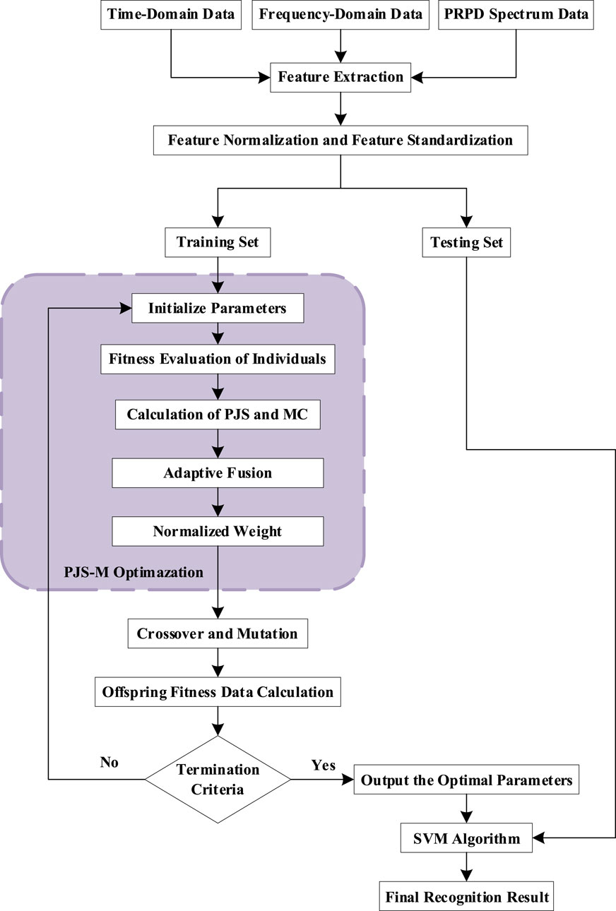
Figure 7. Flowchart for defect-type identification.

6 Recognition results

To verify the effectiveness of the improved algorithm, the recognition accuracy of the proposed GAW-SVM algorithm was compared with that of the GA-SVM, PCA-SVM (Sinha et al., 2025), and PSO-SVM (Li et al., 2024) algorithms using different feature combinations. A summary of the recognition accuracy results is presented in Table 2.

Table 2

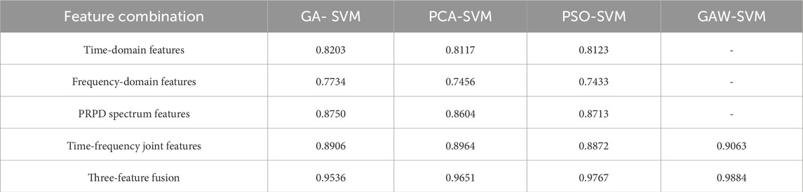
Table 2. Recognition rates of real defect types with different feature combinations (four algorithms).

1. For single-feature identification, since feature fusion is not involved, only the results from the GA-SVM, PCA-SVM, and PSO-SVM algorithms are available. Observations of the data indicate that the overall defect recognition accuracy under single-feature conditions is relatively low. Even for the relatively better-performing PRPD pattern feature, the recognition rate under the GA-parameter-optimized SVM algorithm reaches only 87.50%, indicating suboptimal identification performance. This demonstrates that although single-domain features can be used for real defect identification, their limited characterization capability leads to misclassification in cases of real defects involving multiple PD sources coupled together, as the similarity of signals under a single feature may cause incorrect judgments and consequently lower recognition rates.

2. In the analysis of time–frequency combined feature sets, the recognition accuracies of the four algorithms, ranked from highest to lowest, are as follows: GAW > PCA > GA > PSO. Among them, the GAW-SVM algorithm achieved the highest recognition accuracy at 90.63%, while the PSO-SVM algorithm yielded the lowest at 88.72%. Compared with single-domain features, the time–frequency fusion primarily performs data augmentation on existing features without introducing new representational dimensions, resulting in a limited overall improvement. Nevertheless, the enhanced GAW-SVM still demonstrated superior performance, indicating that the proposed weight optimization strategy effectively improves defect classification capability.

3. In the multi-source, three-feature fusion analysis, the proposed GAW-SVM achieved the highest defect-recognition accuracy (98.84%), followed by PSO-SVM (97.67%), PCA-SVM (96.51%), and GA-SVM (95.35%). These results demonstrate that multi-source, multi-feature fusion markedly improves overall recognition performance. Compared with single-source time-frequency fusion, the multi-source, multi-feature approach increased accuracy for GA, PCA, PSO, and GAW classifiers by 6.29%, 6.87%, 8.95%, and 8.21%, respectively. Moreover, the GAW-SVM outperformed GA-SVM, PCA-SVM, and PSO-SVM by 3.49%, 2.33%, and 1.17%, respectively, further confirming the effectiveness of the proposed improvements for identifying real-world cable-joint defects. These findings indicate that multi-source, multi-feature fusion is a superior strategy for real-defect identification, overcoming the misclassification errors that arise when single-source features are used for complex defects. In particular, the inclusion of the PJS-M weighting coefficient and correlation-analysis–based dynamic correction mechanism in the GAW-SVM framework substantially enhances recognition accuracy for fused multi-feature datasets.

7 Conclusion

In this study, the traditional GA-SVM algorithm was improved using the PJS-M method, and the defect recognition performance for real-type defects was enhanced through multi-sensor fusion–based identification.The main conclusions drawn from the study findings are as follows.

1. The time-domain waveforms of the three types of real defects selected in this study exhibit varying degrees of differences in discharge amplitude, symmetry between the positive and negative half-axes, and decay rate. Differences in the frequency-domain spectra are primarily reflected in frequency bandwidth, spectral energy, and spectral peak characteristics. The PRPD patterns differ in discharge phase, amplitude, discharge concentration, and overall pattern morphology. From the PRPD patterns, it is visually evident that there are distinct contour differences between the patterns of real defects and those of typical defects. This indicates that the research on real defect identification conducted in this study holds practical value for applications in industrial production.

2. Compared with the highest-performing single-domain feature—PRPD feature-based recognition—the multi-source and multi-feature fusion approach achieved recognition accuracy improvements of 7.85%, 10.47%, and 10.54% under the GA-SVM, PCA-SVM, and PSO-SVM algorithms, respectively. Furthermore, relative to single-source multi-feature fusion, the recognition accuracies were enhanced by 6.29%, 6.87%, 8.95%, and 8.21% across the GA-SVM, PCA-SVM, PSO-SVM, and GAW-SVM algorithms, respectively. This indicates that multi-source fusion identification can overcome the limitations of incomplete characterization of real defects caused by relying solely on single-domain features or single-source features.

3. This study integrates non-homogeneously acquired features from the time domain, frequency domain, and phase-resolved partial discharge (PRPD) patterns, and incorporates a Probabilistic Jensen–Shannon Margin (PJS-M) adaptive weighting mechanism into the GA-SVM framework. By combining data-driven and model-driven dual-weighting strategies, the proposed approach effectively leverages the complementary information among heterogeneous feature types, mitigates model overfitting, and improves the utilization efficiency of multi-source fused features. The resulting improved GAW-SVM algorithm achieves a defect recognition accuracy of 98.84%, demonstrating superior discriminative capability for complex real-type defects compared to other benchmark algorithms. This research provides a reliable basis and technical reference for partial discharge detection in cable intermediate joints, offering significant value for practical engineering applications.

4. Existing studies have shown that slight variations in cavity dimension, shape, and position can affect the characteristics of PD pulses, potentially influencing feature extraction and the performance of classification models. However, due to experimental limitations, this study was unable to perform data acquisition and comparative analysis for defects of different sizes during the experimental process. Therefore, future experimental research could include such control groups to further expand the practical applicability of the method proposed in this study.

Data availability statement

The raw data supporting the conclusions of this article will be made available by the authors, without undue reservation.

Author contributions

L-XZ: Funding acquisition, Investigation, Supervision, Writing – review and editing, Writing – original draft, Software, Data curation, Project administration, Validation, Resources, Conceptualization, Methodology, Visualization, Formal Analysis. Y-YZ: Investigation, Conceptualization, Software, Writing – review and editing, Methodology. S-JY: Methodology, Project administration, Writing – review and editing, Supervision. J-LC: Methodology, Supervision, Writing – review and editing, Project administration. Y-JC: Writing – review and editing, Data curation, Investigation. Z-SZ: Writing – review and editing, Formal Analysis, Project administration, Validation, Supervision, Methodology, Visualization, Investigation, Conceptualization.

Funding

The author(s) declare that no financial support was received for the research and/or publication of this article.

Acknowledgments

The author is grateful for the support of all colleagues at the Pingliang Road Laboratory of Shanghai University of Electric Power.

Conflict of interest

The authors declare that the research was conducted in the absence of any commercial or financial relationships that could be construed as a potential conflict of interest.

Generative AI statement

The author(s) declare that no Generative AI was used in the creation of this manuscript.

Any alternative text (alt text) provided alongside figures in this article has been generated by Frontiers with the support of artificial intelligence and reasonable efforts have been made to ensure accuracy, including review by the authors wherever possible. If you identify any issues, please contact us.

Publisher’s note

All claims expressed in this article are solely those of the authors and do not necessarily represent those of their affiliated organizations, or those of the publisher, the editors and the reviewers. Any product that may be evaluated in this article, or claim that may be made by its manufacturer, is not guaranteed or endorsed by the publisher.

Supplementary material

The Supplementary Material for this article can be found online at: https://www.frontiersin.org/articles/10.3389/fenrg.2025.1622318/full#supplementary-material

References

Bo, N., Feiyue, M., Xutao, W., Ni, H., Zhou, X., and Wu, H. (2022). Research and application of intermittent partial discharge characteristics and easy-warning system for electric equipment. Energy Rep. 8 (S10), 217–226. doi:10.1016/j.egyr.2022.05.150

CrossRef Full Text | Google Scholar

Cavallini, A., Montanari, G. C., Puletti, F., and Contin, A. (2005). A new methodology for the identification of PD in electrical apparatus: properties and applications. IEEE Trans. Dielectr. Electr. Insulation 12 (2), 203–215. doi:10.1109/tdei.2005.1430391

CrossRef Full Text | Google Scholar

Chang, C. K., Chang, H. H., and Boyanapalli, B. K. (2022). Application of pulse sequence partial discharge based convolutional neural network in pattern recognition for underground cable joints. IEEE Trans. Dielectr. Electr. Insulation 29 (3), 1070–1078. doi:10.1109/tdei.2022.3168328

CrossRef Full Text | Google Scholar

Chen, X., Shao, X., Pan, X., Luo, G., Bi, M., Jiang, T., et al. (2022). Feature extraction of partial discharge in low-temperature composite insulation based on VMD-MSE-IF. CAAI Trans. Intell. Technol. 7 (2), 301–312. doi:10.1049/cit2.12087

CrossRef Full Text | Google Scholar

Deb, K., Pratap, A., Agarwal, S., and Meyarivan, T. (2002). A fast and elitist multiobjective genetic algorithm: NSGA-II. IEEE Trans. Evol. Comput. 6 (2), 182–197. doi:10.1109/4235.996017

CrossRef Full Text | Google Scholar

Guohai, L. I. U., Lingling, Chen, Wenxiang, Zhao, Jiang, Y., and Qu, L. (2013). Internal model control of permanent magnet synchronous motor using support vector machine generalized inverse. IEEE Trans. Industrial Inf. 9 (2), 890–898. doi:10.1109/tii.2012.2222652

CrossRef Full Text | Google Scholar

Haralick, R. M., Shanmugam, K., and Dinstein, I. (1973). Textural features for image classification. IEEE Trans. Syst. Man, Cybern. SMC-3 (6), 610–621. doi:10.1109/tsmc.1973.4309314

CrossRef Full Text | Google Scholar

Hu, M. K. (1962). Visual pattern recognition by moment invariants. IRE Trans. Inf. Theory 8 (2), 179–187. doi:10.1109/TIT.1962.1057692

CrossRef Full Text | Google Scholar

Jiao, J., and Jie, L. I. (2023). Cable terminal defect diagnosis method based on improved residual network. Electr. DRIVE 53 (11), 31–36. doi:10.19457/j.1001-2095.dqcd24464

CrossRef Full Text | Google Scholar

Korobeynikov, S. M., Ridel, A. V., Karpov, D. I., Ovsyannikov, A. G., and Meredova, M. B. (2019). Mechanism of partial discharges in free helium bubbles in transformer oil. IEEE Trans. Dielectr. Electr. Insulation 26(5), 1605–1611. doi:10.1109/tdei.2019.008199

CrossRef Full Text | Google Scholar

Li, X., Yang, H., Ge, J., Zhu, S., and Zhu, Z. (2024). Intelligent cavitation recognition of a canned motor pump based on a CEEMDAN-KPCA and PSO-SVM method. IEEE Sensors J. 24 (4), 5324–5334. doi:10.1109/jsen.2023.3347248

CrossRef Full Text | Google Scholar

Liu, Y., Liu, H., and Zhang, P. (2022). Analysis of ultraviolet imaging detection in external detection of substation equipment. J. Opt. 51 (4), 1071–1077. doi:10.1007/s12596-022-00840-0

CrossRef Full Text | Google Scholar

Mingyu, M., and Wang, W. (2022). Transformer fault diagnosis based on improved support vector machine. Zhengzhou, China: North China University of Water Resources and Electric Power.

Google Scholar

Rostaminia, R., Saniei, M., Vakilian, M., Mortazavi, S. S., and Parvin, V. (2016). Accurate power transformer PD pattern recognition via its model. IET Sci. Meas. and Technol. 10 (7), 745–753. doi:10.1049/iet-smt.2016.0075

CrossRef Full Text | Google Scholar

Shang, H., Kwok, L., and Feng, Li (2017). Partial discharge feature extraction based on ensemble empirical mode decomposition and sample entropy. Entropy 19 (9), 439–457. doi:10.3390/e19090439

CrossRef Full Text | Google Scholar

Sinha, P., Paul, K., and Mohanty, A. (2025). Efficient automated detection of power quality disturbances using nonsubsampled contourlet transform and PCA-SVM. Energy Explor. and Exploitation 43 (3), 1149–1179. doi:10.1177/01445987241312755

CrossRef Full Text | Google Scholar

Sitong, L. I., Qiang, Zhuang, and Lin, J. I. N. (2018). Partial discharge pattern recognition method based on time-frequency characteristic kernel entropy component analysis. High. Volt. Appar. 54 (6), 125–131. doi:10.13296/j.1001-1609.hva.2018.06.019

CrossRef Full Text | Google Scholar

Wojciech, S., and Artur, W. (2023). Low-cost online partial discharge monitoring system for power transformers. Sensors Basel, Switz. 23 (7), 3405. doi:10.3390/s23073405

CrossRef Full Text | Google Scholar

Wu, J. (2014). Fault recognition method research based on the wavelet energy spectrum of mode components. Xian: Xian University of Science and Technology.

Google Scholar

Yang, M. (2006). Research on pattern recognition of PD in oil-paper insulation based on statistical and fractal feature. Chongqing: Chongqing University.

Google Scholar

Yekun, M. E. N., Pan, Z., and Liu, B. (2024). Defect recognition of distribution power cable through harmonic analysis of grounding current. Proc. CSU-EPSA 36 (07), 116–121. doi:10.19635/j.cnki.csu-epsa.001374

CrossRef Full Text | Google Scholar

Yuanhu, G., Jiabo, C., Mingda, Y., and Shi, K. (2023). Online intelligent temperature monitoring system for tunnel power cable based on fiber bragg grating. J. Phys. Conf. Ser. 2465 (1), 012038. doi:10.1088/1742-6596/2465/1/012038

CrossRef Full Text | Google Scholar

Yunfeng, L., Ziwen, C., and Wenpeng, L. (2025). “Analog circuit fault diagnosis algorithm based on KPCA feature optimization combined with improved GA-SVM,” in 2025 10th Asia conference on power and electrical engineering (ACPEE). IEEE, 915–921.

CrossRef Full Text | Google Scholar

Zhao, W., Lv, Y., and Xiao, J. (2021). Fault diagnosis of rolling bearings based on GA-SVM model.2021 global reliability and prognostics and health management (PHM-Nanjing). IEEE, 1–6. doi:10.1109/PHM-Nanjing52125.2021.9612886

CrossRef Full Text | Google Scholar

Zhu, H., and Shen, L. (2024). Decoupling control of outer rotor coreless bearingless permanent magnet synchronous generator using LS-SVM inverse system optimized by the improved genetic algorithm. Proc. CSEE 44 (05), 2037–2047. doi:10.13334/j.0258-8013.pcsee.222640

CrossRef Full Text | Google Scholar