An optimal reactive power pre-dispatch approach for minimizing active power losses

Renewable energy sources (RES) depend on location and weather conditions, which can negatively impact the transmission system operator’s active power losses. This paper proposes a method that operates between the day-ahead market clearing and real-time operation. It enables transmission system operators (TSOs) to procure supplemental reactive power from generator companies (GenCos) in order to minimize active power losses. To achieve this, a multi-objective, bi-level optimization model is proposed. The leader’s goal is to find a fair reactive power price that leads to the best trade-off between the two conflicting objectives of maximizing the savings for the TSO and the extra reactive power income for GenCos. The follower problem considers an optimal power flow model and minimizes the costs for the TSO by selecting the appropriate control action. The method was evaluated using the Nordic 44 test case. Results indicate a potential price range starting from $\mathbf{0}\text{\hspace{0.17em}\$}/\text{MVarh}$, which is the preferable price for the TSO, up to $\mathit{1.08}\text{\hspace{0.17em}\$}/\text{MVarh}$, representing the best possible price for the GenCos. Using the Tchebycheff scalarization method, the reactive power price of $\mathit{0.28}\text{\hspace{0.17em}\$}/\text{MVarh}$ is found to be the best trade-off for both parties. However, these prices depend on multiple factors related to the case study. Overall, the method can improve the interaction between GenCos and the TSO by proposing a fair remuneration for GenCos, which is still profitable for the TSO.

1 Introduction

1.1 Motivation and problem formulation

Active power losses in transmission lines are caused by the flow of current through the ohmic resistance inherent to each line. They, therefore, depend on the load connected, the associated voltages, and the line resistance. Whereby the resistance increases linearly with the line length.

Renewable energy sources (RES) are constructed in locations that provide high returns for the owner companies and where the geography facilitates their development. Therefore, the locations where the power plants are built are not necessarily where the power is consumed.

In the Nordic grid, for example, many essential hydropower plants are located in the north of Norway and Sweden or the southwest of Norway (Energinet and Kraftnät, 2021). At the same time, the main load centers are situated in the southeast of Norway or in the south of Sweden (Energinet and Kraftnät, 2021). This leads to power flows over long distances to the consumers, resulting in considerable losses even at high voltages.

This challenge is not confined to the Nordic grid; it also applies to the Great Britain transmission system operator, National Grid ESO. According to a report (Transmission, 2019), it is believed that the primary cause of future active losses in its grid is geographically distributed generation.

The fundamental issue that arises from this is that the network operator must purchase the active power losses at the spot market price for the associated hour (Statnett, 2024), which ultimately leads to higher costs for the end consumer (i.e., society).

One solution to reduce losses is to upgrade the existing equipment. However, this leads to considerable investment that often cannot be justified by considering active power losses exclusively; furthermore, local improvements may reduce losses at a particular location while also leading to an overall increase in losses due to changes in power flows (Transmission, 2019). Another measure, explored in this paper, is optimizing reactive power procurement and dispatch to minimize losses by properly coordinating reactive power sources.

Reactive power is unavoidable when transmitting active power, and its inappropriate handling can lead to serious security problems, including stability issues and reduced transfer capacity (El-Samahy et al., 2008). However, reactive power has some specific technical characteristics. The most dominant aspects relevant to this paper are that it does not require fuel for generation, and it cannot be transferred over long distances (Wolgast et al., 2022). Determining the price of reactive power is therefore non-trivial; however, since reactive power is vital for system operation, it also has an associated value that must be determined appropriately. Furthermore, a reactive power price set too low or too high can lead to false incentives and, ultimately, to critical technical issues (Rabiee et al., 2009).

1.2 Literature review

When dealing with optimal reactive power procurement and dispatch, it is essential to determine the temporal specifications, such as when the optimization is executed and based on what data. For example (El-Samahy et al., 2008), proposes procuring the optimal reactive power in a first step on a seasonal basis and later dispatching it shortly before the actual application. Zhang and Ren (2005), on the other hand, follows a more real-time dispatch approach, where it is assumed that the loading conditions are approximately constant over a specific time interval (e.g., 1 h). Time-critical aspects of reactive power redispatch using optimal power flow (OPF) were emphasized and investigated in a specifically tailored real-time laboratory setup in Martín et al. (2024).

This article implements the dispatch optimization algorithm in the period between the closed day-ahead market and real-time application, and therefore refers to it as reactive power pre-dispatch.

Besides the temporal aspects of the reactive power procurement and dispatch approach, the modeling and optimization methods used are also relevant. Many authors model the process using a two-step or bi-level optimization approach, as seen for example in the works (El-Samahy et al., 2008; Bhattacharya and Zhong, 2001; Almeida and Senna, 2011; Almeida et al., 2016). In one level or the first step, they calculate the dual variables that they use later in the upper-level or second step as a price indicator. El-Samahy et al. (2008), Bhattacharya and Zhong (2001) use the duals directly to determine the value of reactive power. While (Bhattacharya and Zhong, 2001) examines sensitivity concerning active power losses, (El-Samahy et al., 2008), also considers security aspects in its optimization process. In the second optimization step, the calculated duals are used to maximize a societal advantage function (SAF). The authors in Almeida and Senna (2011), Almeida et al. (2016), on the other hand, utilize the duals of the follower problem as active power price sensitivities, which are then applied in the leader problem to minimize the opportunity costs. Dual variables also play a role in Feng et al. (2024), where the authors analyze three different scenarios for minimizing active power losses with reactive power support and map these scenarios to dual variable configurations. A stochastic two-stage model was proposed by the authors of Jiang et al. (2022). They present a day-ahead market mechanism for reactive power ancillary services and propose a modified version of the Vickrey-Clark-Groves mechanism, specifically designed for reactive power services in systems with high RES penetration.

Besides generators, the grid owner itself typically has equipment for controlling reactive power flows. The switching action of such reactive power control devices, such as capacitor banks, leads to costs, for example, a reduction in the device’s lifespan. Therefore, Zhang and Ren (2005) proposes to find a trade-off between active power losses and these switching costs. Such costs for reactive power-controlled devices are also considered in the work of Lamont and Fu (1999). The objective of Lamont and Fu (1999) is to dispatch the reactive power of generators as well as the reactive power-controlled equipment to minimize real power losses. The optimal power flow problem is iteratively solved, with the prices for the various reactive sources being calculated and adjusted in each iteration. These prices comprise explicit costs (capital and operating costs) and opportunity costs, utilizing a triangular relationship and probability distribution. The use of the triangular relationship proposed by Lamont and Fu (1999) to determine the value of reactive power was followed by the authors of De and Goswami (2014). Furthermore, De and Goswami (2014) proposed three different formulations of an OPF for reactive power procurement and compared them with two classic formulation approaches, one of which takes into account the L index (first published in (Kessel and Glavitsch, 1986)) to determine the proximity to voltage instability, and the other minimizes system losses. Hao (2003) proposes that generation companies should be obligated to provide reactive power free of charge in proportion to their active power output (an approach already implemented in countries such as Norway Statnett (2022)). In addition, Hao (2003) suggests that any provision of reactive power beyond this proportional obligation should be financially compensated.

This paper adopts a similar principle to that proposed by Hao (2003), but instead considers compensation for any deviation from the initially scheduled reactive power set point. Furthermore, to determine both the optimal change in reactive power set point and the corresponding reactive power price, a strategy hereafter called pre-dispatch is formulated based on a bi-level optimization problem. At the lower level, the objective is to minimize costs related to active power losses, along with costs for supplemental reactive power injections from the generators, which is a relatively standard approach. However, this paper does not utilize the dual variables of the lower-level; instead, it varies the unknown reactive power price within a specific cost interval and calculates the power flow solution for each price separately. The authors chose this method because it enables the analysis of the Pareto front of the two conflicting objectives in the upper-level (leader problem). Consequently, this helps to find the best trade-off between the two objectives in the upper-level problem.

In addition to the modeling and temporal aspects of optimal reactive power dispatch and procurement, the choice of solving strategy often plays an essential role. Several of the optimization models mentioned involve AC power flow equations, resulting in nonlinear and nonconvex optimization problems. If no binary variables are included, techniques such as those used in Lamont and Fu (1999) can be applied. These techniques allow for an iterative solution by linearizing the problem at each step. Another method that can be utilized is semidefinite programming, as discussed in Davoodi et al. (2019). However, a common challenge with conventional solvers is that they may converge to a local minimum (Kumar et al., 2023). To address this issue, many authors apply metaheuristic methods, which can help overcome these limitations and potentially converge to the global minimum. For example, Zhang and Ren (2005), uses a cataclysmic genetic algorithm; (De and Goswami, 2014), on the other hand, uses an artificial bee colony algorithm (Cabezas Soldevilla et al., 2019); uses a particle swarm technique; and the authors of Salimin et al. (2024) present a hybrid algorithm named integrated accelerated clonal evolutionary programming. Enhanced differential evolutionary algorithms are proposed in Kumar et al. (2023), Kar et al. (2023). The performance of the algorithms is compared to other metaheuristics using two statistical analysis methods: the Wilcoxon signed-rank test and the Friedman-Nemenyi statistical test (Kar et al., 2024). proposes a modified whale optimization algorithm for solving the OPF-based optimization problem for minimizing active power losses using FACTS devices.

This paper aims to develop a method for optimal pre-dispatch of reactive power, rather than comparing different solvers with each other. A conventional interior-point method was used here as an example. However, the code is publicly available, including the used power system model (Baltensperger, 2025), and solvers can be modified using the Pyomo environment.

1.3 Objective, contribution and paper organization

The key objective of the proposed method is to reduce the costs for society by lowering active power losses and fairly procuring reactive power from generator companies. For doing so, the paper proposes an optimal pre-dispatch method based on a two-level optimization formulation. The method serves as an intermediary step between day-ahead scheduling and real-time application, enabling the TSO to procure extra reactive power from (GenCos) in order to minimize active power losses. The cash-flow diagram of Figure 1 shows, in the most fundamental way, the objective of the method. The left side illustrates the situation without the proposed reactive power pre-dispatch step, whereas the right side shows the problem with the pre-dispatch step. Without pre-dispatch (left), the TSO pays $\$P_{\mathit{loss,0}}$ for additional active power support of the GenCos due to system losses. With the pre-dispatch step (right), the TSO pays an extra amount of money for supplemental reactive power $\$Q_{\mathit{Cos}}^{\mathit{Gen}}$ (red arrow), intended to reduce the cost for active power losses $\$P_{\mathit{loss,1}}$ (blue arrow). Compared to the situation without the pre-dispatch step, reducing active power losses leads to extra income for GenCos since reactive power is now remunerated ($\$Q_{\mathit{Cos}}^{\mathit{Gen}}$). However, it also reduces revenues from active power support as written in (Equation 1).

$\$P_{\mathit{Rev.Red.}}^{\mathit{GenCos}}=\mathrm{\Delta }\$P_{\mathrm{0,1}}=\$P_{\mathit{loss,0}}-\$P_{\mathit{loss,1}}(1)$

${\$}_{\mathit{Tot.Cost}}^{\mathit{TSO,0}}=\$P_{\mathit{loss,0}},{\text{\$}}_{\mathit{Tot.Cost}}^{\mathit{TSO,1}}=\$P_{\mathit{loss,1}}+\$Q_{\mathit{Cos}}^{\mathit{Gen}}(2)$

${\$}_{\mathit{Saving}}^{\mathit{TSO}}=\mathrm{\Delta }\$P_{\mathrm{0,1}}-\$Q_{\mathit{Cos}}^{\mathit{Gen}}={\text{\$}}_{\mathit{Tot.Cost}}^{\mathit{TSO,0}}-{\text{\$}}_{\mathit{Tot.Cost}}^{\mathit{TSO,1}}(3)$

From a TSO point of view, the total costs include not only the expenses for active power losses but also the extra costs associated with reactive power, as it is written in (Equation 2). Therefore, the savings for the TSO can be defined as the difference in total costs between the situation without and with the pre-dispatch step as written in (Equation 3).

Figure 1

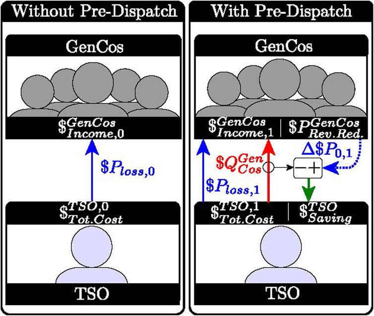
Figure 1. Fundamental idea and objective of the proposed pre-dispatch process.

When discussing optimal pre-dispatch, it is necessary to address the meaning of ‘‘optimal’ specifically. With ‘optimal’ pre-dispatch, the objective is to determine a new price for supplemental reactive power, represented as $c_g^{*}$, that reduces the active power losses and maximizes the savings for the TSO $({\text{\$}}_{\mathit{Saving}}^{\mathit{TSO}})$ and reactive power income of the GenCos $(\$Q_{\mathit{Cos}}^{\mathit{Gen}})$. These two objectives are conflicting as written in (Equation 3).

In the context of the mentioned pre-dispatch strategy, this paper addresses two key research questions:

1. What is the reasonable economic value of reactive power when considering active power losses?

2. What is the most equitable price for reactive power that considers all parties involved?

1.3.1 Contributions

• Method addressing TSO and GenCos needs: A method has been proposed for the pre-dispatch of reactive power, allowing the TSO to procure reactive power to minimize active power losses. The novelty of the suggested method lies in its capacity to consider the requirements of both the TSO and the GenCos to the greatest extent possible.

• Pricing procedure: For determining the economic value of reactive power, a multi-objective, bi-level optimization model is selected, which allows the determination of a fair trade-off between the savings of the TSO due to the minimization of active power losses and the supplemental reactive power income of the GenCos.

The remainder of the paper is structured as follows: Section 2 details the method and solving strategy used. Section 3 presents the test model along with simulation results. Sections 4, 5 provide a discussion of the results and the conclusions drawn. All relevant variables and their meanings are summarized in Table 1.

Table 1

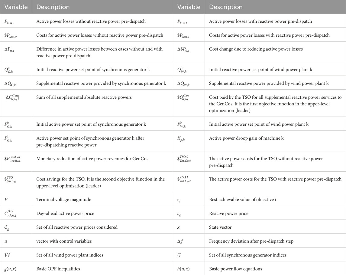
Table 1. Overview of the most relevant variables.

2 Methods

The primary algorithm discussed in this paper is specifically focused on the blue-bordered block labeled “pre-dispatch” illustrated in Figure 2. The green block’s primary purpose is to allocate resources by determining $P_G^0$ and $Q_G^0$. It can be regarded as an initial estimate of the active power losses calculated by the TSO on the basis of the day-ahead market result.

Figure 2

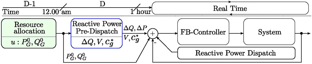
Figure 2. The conceptual idea. The green block represents the TSO’s resource allocation based on the results from the power market. The blue-bordered block contains the main content of this paper. “FB-Controller” refers to the feedback controllers applied to the system in real time.

Based on the output of the resource allocation block, the pre-dispatch block minimizes active power losses with the proposed optimization technique. As shown in Figure 2, the pre-dispatch step occurs between the clearing of the day-ahead market and the real-time application. The loads are expected to be static, as scheduled in the day-ahead market. Therefore, the optimization must be performed for each time interval defined by the day-ahead market structure, typically hourly or every 15 min. Once the set points are computed and the corresponding time interval is reached during real-time operation, the optimized set points are applied to the system. If the scheduled load or generation does not match in real time, the balancing market will intervene. It should be mentioned at that point that the optimizer keeps the active power set point unchanged. Consequently, no opportunity costs are taken into account. The change in active power resulting from the savings achieved by minimizing active power losses is modeled using a distributed slack bus. In addition to the set points, the pre-dispatch block outputs the reactive power price per MVarh, where $c_g^{*}$ represents the optimal economic value of the supplemental reactive power used to minimize active power losses.

The mathematical idea of the pre-dispatch block proposed in this paper is formulated as a bi-level problem, as stated in (Equations 4–7).

$\underset{c_g}{\max }\left(\begin{array}{c}\hfill \$Q_{\mathit{Cos}}^{\mathit{Gen}}\left(u\left(c_g\right),x\left(c_g\right),c_g\right)\hfill \\ \hfill {\text{\$}}_{\mathit{Saving}}^{\mathit{TSO}}\left(u\left(c_g\right),x\left(c_g\right),c_g\right)\hfill \end{array}\right)(4)$

$\text{s.t.}\left(u\left(c_g\right),x\left(c_g\right)\right)\in \arg \underset{u,x}{\min }\left({\text{\$}}_{\mathit{Tot.Cost}}^{\mathit{TSO,1}}\left(u,x,c_g\right)\right)(5)$

$\text{s.t.}g\left(u,x,c_g\right)\le 0(6)$

$h\left(u,x,c_g\right)=0(7)$

The main goal of the follower problem (Equations 5–7) is to minimize the total cost for the TSO (${\text{\$}}_{\mathit{Tot.Cost}}^{\mathit{TSO,1}}$), which is the costs for active power losses and supplemental reactive power services. This is achieved by selecting the optimal vector for the control variables $u$ and the state vector $x$, with the OPF being parametrized by a price $c_g$. Equation 6 represents basic inequality constraints used in an OPF, such as the minimum and maximum limits of the nodal voltage magnitudes. Equation 7 includes the fundamental power flow equations.

On the other hand, the leader problem is multi-objective. It aims to determine the best price for additional reactive power $c_g$, maximizing savings for the TSO (${\text{\$}}_{\mathit{Saving}}^{\mathit{TSO}}$) and income for supplemental reactive power services for the GenCos ($\$Q_{\mathit{Cos}}^{\mathit{Gen}}$), as it is written in Equation 4.

The optimization method can be described in simple terms. Essentially, the price of reactive power $c_g$ is varied, and an OPF is calculated for each price point. The results of these calculations are then compared against the objectives of the GenCos and the TSO at the upper level. This process allows for an analysis of the trade-offs between the objectives of the GenCos and the TSO.

The following subsections discuss how this framework is modeled and solved in detail.

2.1 Modeling the follower problem

Besides the objective function, the follower optimization model used in this paper is a classical OPF written in a general form in (8).

$\begin{array}{cc}\hfill & \left(u\left(c_g\right),x\left(c_g\right)\right)=\underset{u,x}{\mathrm{arg\; min}}\stackrel{\$P_{\mathit{loss,1}}\left(u,x,c_g\right)}{\overbrace{C_{\mathit{Ahead}}^{\mathit{Day}}{P}_{\mathit{loss,1}}}}+{\displaystyle \stackrel{\$Q_{\mathit{Cos}}^{\mathit{Gen}}\left(u,x,c_g\right)}{{\displaystyle \overbrace{c_g{\displaystyle \underset{|\mathrm{\Delta }{Q}_{\mathit{Cos}}^{\mathit{Gen}}|}{{\displaystyle \underbrace{\left({\displaystyle \sum _{k\in \mathcal{G}}}|\mathrm{\Delta }{Q}_{G,k}|+{\displaystyle \sum _{k\in \mathcal{W}}}|\mathrm{\Delta }{Q}_{W,k}|\right)}}}}}}}}\hfill \\ \hfill & \text{s.t.}g\left(u,x\right)\le 0,h\left(u,x\right)=0\hfill \end{array}(8)$

The objective function contains the costs for active power losses in the transmission lines $\$P_{\mathit{loss,1}}$ and the income of supplemental reactive power of the GenCos willing to participate in the pre-dispatch service $\$Q_{\mathit{Cos}}^{\mathit{Gen}}$. At this point, clarifying the meaning of some variables is essential. $|\mathrm{\Delta }{Q}_{\mathit{Cos}}^{\mathit{Gen}}|$ represents the supplemental reactive power provided by the GenCos that compensates for active power losses. The sets $\mathcal{G}$ and $\mathcal{W}$ consist of all synchronous machines and wind turbines of the GenCos that participate in the pre-dispatch service.

The vector $x$ contains all states, such as nodal voltage magnitudes at load buses, and $u$ is the vector with all control variables, for example, generator terminal voltages. In the given problem, $C_{\mathit{Ahead}}^{\mathit{Day}}$ is the active power price (e.g., the day-ahead price) used to consider the losses in terms of costs. $c_g$ is the decision variable of the leader problem and represents the price for supplemental reactive power. The constraints $g(u,x)$ represent the set of inequalities such as line-flow limits, and $h(u,x)$ are, for example, power flow equations.

The modeling aspects of the reactive power sources considered in the OPF are explained below. However, a more detailed description of the fundamental aspects of conventional OPFs, such as written in (Equation 8), is not provided as it is commonly known. For more information on this topic, the reader is referred to the relevant literature such as Conejo and Baringo (2018).

2.1.1 Synchronous machines

All synchronous machines are modeled as round-rotor machines following the capability curve illustrated in Figure 3. Each machine out of the set $\mathcal{G}$ is modeled with the constraints shown in (Equations 9–13).

Figure 3

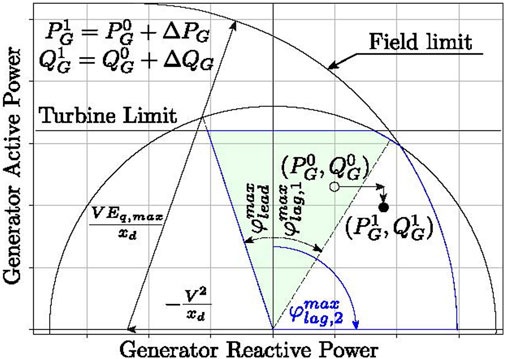
Figure 3. Capability curve of round-rotor synchronous machines. Superscript 0 describes the set points determined in the allocation block, and superscript 1 is the final set points applied to the system.

The delta reactive power output $\mathrm{\Delta }{Q}_G$, the active and apparent power output after the pre-dispatch step $(P_G^1,S_G^1)$ are state variables. At the same time, the generator terminal voltage $V$ is the control variable.

Considering (Equation 11), the maximum machine apparent power output is assumed to be constant and not dependent on the terminal voltage. The turbine limit represents the upper active power limit (see (Equation 10)). The resource allocation algorithm used by the TSO in the first green block shown in Figure 2 selects the set points from the light green area, whereas the pre-dispatch optimizer can choose set points from the blue-bordered area of the capability curve depicted in Figure 3. As the associated grid code dictates, the green area represents a power factor between 0.86 (capacitive) and 0.95 (inductive). The pre-dispatch optimization procedure has relaxed restrictions, allowing the optimizer more freedom to select the suitable set points to minimize losses. Since the pre-dispatch optimization problem minimizes active power losses, there will consequently be a change in the active power set point of the machines that are implemented based on the policy of a distributed slack bus as it is written in (Equation 9). It is essential to understand that the optimizer cannot simply choose the active power set point to minimize losses. The only permissible adjustment is made through the distributed slack, which is used solely to appropriately compensate for the new active power losses due to changes in terminal voltage and reactive power set points. The field current limit is assumed to depend on the terminal voltage and the quadrature component’s internal voltage behind the EMF, as described in Machowski et al. (2020), written in (Equation 13) and illustrated in Figure 3. The synchronous reactance is assumed to be equal for all machines connected ($x_d=2.23p.u$.). The constraints for absorbing reactive power are written in Equation 12.

$P_{G,k}^1=P_{G,k}^0-K_{p,k}\mathrm{\Delta }f\forall k\in \mathcal{G}(9)$

$P_{G,k}^{\mathit{min}}\le P_{G,k}^1\le P_{G,k}^{\mathit{max}}\forall k\in \mathcal{G}(10)$

$0\le \sqrt{{\left(P_{G,k}^1\right)}^2+{\left(Q_{G,k}^0+\mathrm{\Delta }{Q}_{G,k}\right)}^2}\le S_{G,k}^{\mathit{max}}\forall k\in \mathcal{G}(11)$

$-P_{G,k}^1\tan \left({\phi }_{\mathit{lead}}^{\mathit{max}}\right)\le Q_{G,k}^0+\mathrm{\Delta }{Q}_{G,k}(12)$

$0\le {\left(P_{G,k}^1\right)}^2+{\left(Q_{G,k}^0+\mathrm{\Delta }{Q}_{G,k}+\frac{V^2}{x_d}\right)}^2\le {\left(\frac{V{E}_{q,max}}{x_d}\right)}^2(13)$

2.1.2 Wind power plants

In this paper, the reactive power output of a wind power plant is modeled in such a way that, firstly, the active power remains constant, and, in this respect, the reactive power must be chosen so that the power factor of each plant is between 0.85 (capacitive) and 0.95 (inductive). Equations 14, 15 describe the used constraint for each plant in the optimization model.

$-P_{W,k}^0\tan \left({\cos }^{-1}\left(0.95\right)\right)\le Q_{W,k}^0+\mathrm{\Delta }{Q}_{W,k}\forall k\in \mathcal{W}(14)$

$Q_{W,k}^0+\mathrm{\Delta }{Q}_{W,k}\le P_{W,k}^0\tan \left({\cos }^{-1}\left(0.85\right)\right)\forall k\in \mathcal{W}(15)$

2.2 Modeling the leader problem

The leader problem model, as stated in (Equation 4), aims to maximize the TSO’s savings (${\text{\$}}_{\mathit{Saving}}^{\mathit{TSO}}$) and the GenCos supplemental reactive power income ($\$Q_{\mathit{Cos}}^{\mathit{Gen}}$). Therefore, it is modeled as a multi-objective problem and is solved here using the Tchebycheff scalarization method as described, for example, in Pardalos et al. (2017). The aspects relevant to understanding the definitions, approaches, and scalarization method are briefly explained in this section.

The fundamental idea of the Tchebycheff scalarization method is first to define a so-called utopia point. In literature, the utopia point is defined as a point slightly better than the best achievable value (i.e., $z_i<{\text{min}}_{c_g\in {\mathcal{C}}_g}{f}_i(c_g)$) (Pardalos et al., 2017; Eichfelder, 2008). To be consistent with the literature, the two utopia points are defined here as written in (Equations 16) and (17), where $ϵ$ is set to 1.001 to make sure that the utopia point is not on the solution of the vector-valued objective function:

$z_1=\left(\underset{c_g\in {\mathcal{C}}_g}{\max }\$Q_{\mathit{Cos}}^{\mathit{Gen}}\left(u\left(c_g\right),x\left(c_g\right),c_g\right)\right)\cdot ϵ(16)$

$z_2=\left(\underset{c_g\in {\mathcal{C}}_g}{\max }{\text{\$}}_{\mathit{Saving}}^{\mathit{TSO}}\left(u\left(c_g\right),x\left(c_g\right),c_g\right)\right)\cdot ϵ(17)$

The point $(z_1,z_2)$ is fictitious because the two goals are in conflict and cannot therefore be reached together. The set ${\mathcal{C}}_g$ includes all considered prices and will be explained in more detail in Section 2.3.

Taking into account the defined utopia point, the best possible compromise of both functions can be found using the calculation, according to Tchebycheff, written in (Equation 18):

$\begin{array}{l}\hfill \underset{c_g\in {\mathcal{C}}_g}{\min }\max \left\{w_1\left(\$Q_{\mathit{Cos}}^{\mathit{Gen}}\left(u\left(c_g\right),x\left(c_g\right),c_g\right)-z_1\right),\right.\\ \hfill \left.w_2\left({\text{\$}}_{\mathit{Saving}}^{\mathit{TSO}}\left(u\left(c_g\right),x\left(c_g\right),c_g\right)-z_2\right)\right\}\end{array}(18)$

This paper sets weights $w_1$ and $w_2$ equally to avoid any preference between the objectives.

2.3 Solving procedure

This section is devoted to the method used to solve the presented multi-objective bi-level problem. First, the effect of the two special prices $(c_g=0)$ and $(c_g=\infty )$ on the follower optimization problem is examined.

Equation 19 shows the follower problem for the case $(c_g=0)$. It is apriori clear that the OPF would minimize the losses optimally since supplemental reactive support of GenCos is free. Therefore, it can be concluded that $(P_{\mathit{loss,1}}\le P_{\mathit{loss,0}})$ and $(\$Q_{\mathit{Cos}}^{\mathit{Gen}}=0)$.

$\begin{array}{l}\hfill \underset{c_g\to 0}{\lim }\underset{u,x}{\mathrm{arg\; min}}\left(C_{\mathit{Ahead}}^{\mathit{Day}}\underset{\le P_{\mathit{loss,0}}}{\underbrace{\left(P_{\mathit{loss,1}}\right)}}+\underset{0}{\underbrace{c_g}}\underset{\ge 0}{\underbrace{\left|\mathrm{\Delta }{Q}_{\mathit{Cos}}^{\mathit{Gen}}\right|}}\right),\\ \hfill \text{s.t.}g\left(u,x\right)\le 0,h\left(u,x\right)=0\end{array}(19)$

The second extreme case is the price $(c_g=\infty )$, represented in (Equation 20). In this case, the OPF would choose the opposite since any extra reactive power would lead to extremely high prices. The OPF now chooses $(|\mathrm{\Delta }{Q}_{\mathit{Cos}}^{\mathit{Gen}}|=0)$, which would lead to $(P_{\mathit{loss,0}}=P_{\mathit{loss,1}})$ and ($\$Q_{\mathit{Cos}}^{\mathit{Gen}}=0$). Therefore, in both cases, ($c_g=0$), and ($c_g=\infty$) would lead to no extra income for the GenCos, which will be suboptimal for the leader problem.

$\begin{array}{l}\hfill \underset{c_g\to \infty }{\lim }\underset{u,x}{\mathrm{arg\; min}}\left(C_{\mathit{Ahead}}^{\mathit{Day}}\underset{P_{\mathit{loss,0}}}{\underbrace{\left(P_{\mathit{loss,1}}\right)}}+\underset{\infty }{\underbrace{c_g}}\underset{0}{\underbrace{\left|\mathrm{\Delta }{Q}_{\mathit{Cos}}^{\mathit{Gen}}\right|}}\right),\\ \hfill \text{s.t.}g\left(u,x\right)\le 0,h\left(u,x\right)=0\end{array}(20)$

Consequently, it is essential to find the interval between these two boundaries where the cost for additional reactive power $\$Q_{\mathit{Cos}}^{\mathit{Gen}}$ is larger than zero. Moreover, finding the largest cost-value $\$Q_{\mathit{Cos}}^{\mathit{Gen}}$ will be relevant for the utopia point $z_1$.

The proposed procedure for solving the problem is shown in the flowchart in Figure 4. The first step in the pre-dispatch block is to initialize five list variables ${\tilde{C}}_g,\tilde{U},\tilde{X},\widetilde{\$}{Q}_{\mathit{Cos}}^{\mathit{Gen}}$ and ${\widetilde{\$}}_{\mathit{Saving}}^{\mathit{TSO}}$. The second step is to solve the follower OPF problem using the parameters $Q_G^0$, $P_G^0$, and the reactive power price $c_g$. The resulting control and state vectors $u_{cg}$, $x_{cg}$ are stored in the list $\tilde{U}$ and $\tilde{X}$, and the reactive power price is updated by incrementally increasing the previous price by $\delta$. This process is repeated until $|\mathrm{\Delta }{Q}_{\mathit{Cos}}^{\mathit{Gen}}|$ becomes zero. The set ${\mathcal{C}}_g$ includes all price values for which $0<|\mathrm{\Delta }{Q}_{\mathit{Cos}}^{\mathit{Gen}}|$.

Figure 4

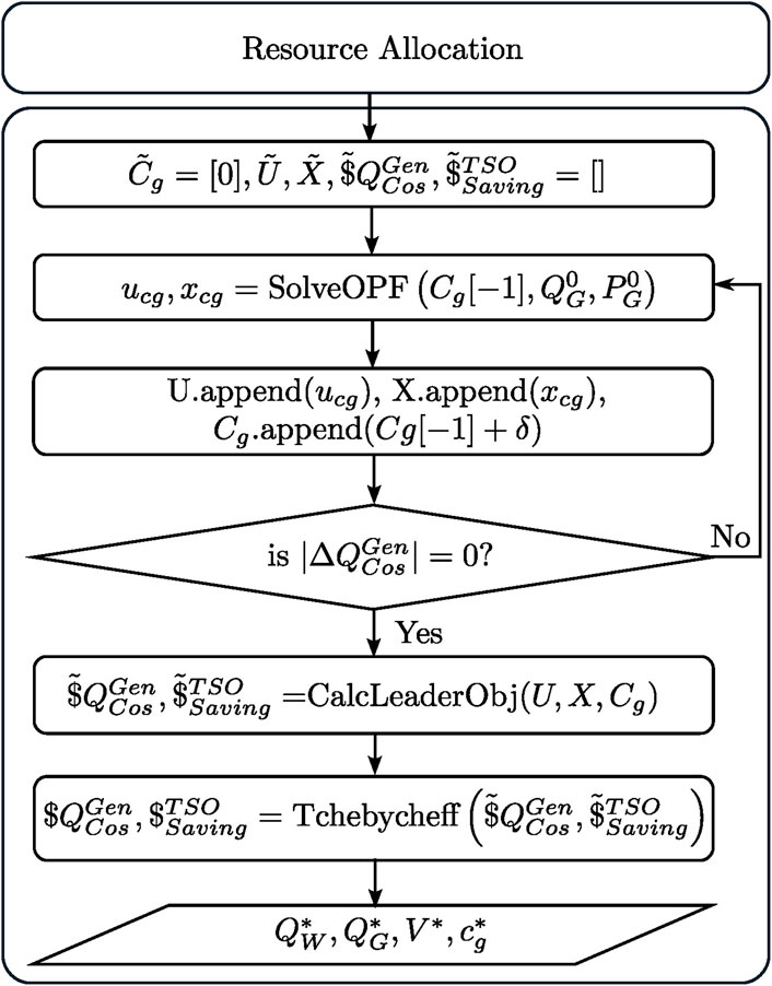
Figure 4. Flowchart of the solving procedure.

The objective function values of the leader problem are computed for all previously obtained solutions at each price in ${\mathcal{C}}_g$, and these values are stored in the two lists $\widetilde{\$}{Q}_{\mathit{Cos}}^{\mathit{Gen}}$ and ${\widetilde{\$}}_{\mathit{Saving}}^{\mathit{TSO}}$. Finally, the best trade-off in the two-objective function of the leader problem is computed using the Tchebycheff scaling method.

3 Test model and simulation results

The model used for testing the proposed technique is the Nordic 44, which can be found in its original form in Jakobsen (2018). The model simplifies the Nordic grid and is today a benchmark for this region. The original model has been slightly modified for this article. To ensure comprehensibility, the full code of the optimizer and the used model is available on GitHub (Baltensperger, 2025).

The optimization in the resource allocation block (green) in Figure 2 is implemented to minimize the generator’s reactive power output.

The results presented here are based on a day-ahead price of $C_{\mathit{Ahead}}^{\mathit{Day}}=70\$/MWh$ (a rule of thumb in the Nordics), which is used for calculating the costs of active power losses.

Figure 5 depicts the active power losses $P_{\mathit{loss,1}}$ and supplemental reactive power $|\mathrm{\Delta }{Q}_{\mathit{Cos}}^{\mathit{Gen}}|$ determined by the optimizer. The left y-axis graph (blue) shows how the active power losses $P_{\mathit{loss,1}}$ change with the price $c_g$. Similarly, the right y-axis graph (red) shows the additional reactive power support $|\mathrm{\Delta }{Q}_{\mathit{Cos}}^{\mathit{Gen}}|$ needed to reduce the losses accordingly. As described in Section 2.2, for $c_g=0$, the reactive power support is maximal, and therefore, the active power losses are minimal. Increasing the price decreases the reactive power support until it reaches zero when the exit criteria of the loop in the flowchart of Figure 4 becomes true. The active power losses increase until they reach the initially observed active power losses $P_{\mathit{loss,0}}$.

Figure 5

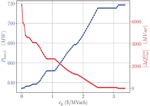
Figure 5. Transmission losses (blue) and reactive power support (red) plotted over reactive power price.

Figure 6 shows the results of the vector-valued objective function of the leader problem. The black trajectory illustrates the objective function values for all considered prices $(c_g\in {\mathcal{C}}_g)$. The green points indicate the Pareto front and the red star is the optimal solution according to the Tchebycheff scalarization. The x-axis represents the objective for the GenCos, and the y-axis represents the objective for the TSO.

Figure 6

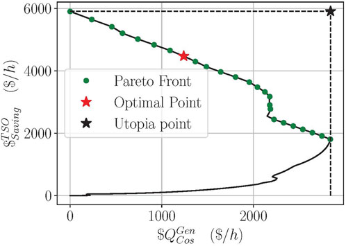
Figure 6. Vector-valued function of the leader objective (black), Pareto front (green), utopia point (black star) and optimal trade-off (red star).

Figure 7 shows the behavior of the costs for supplementary reactive power $\$Q_{\mathit{Cos}}^{\mathit{Gen}}$ (red) and the costs for active power losses $\$P_{\mathit{loss,1}}$ (blue). The green curve in the top subplot represents the savings for the TSO, denoted as ${\text{\$}}_{\mathit{Saving}}^{\mathit{TSO}}$. This curve reaches its maximum at $c_g=0$, indicating the optimal outcome for the TSO.

Figure 7

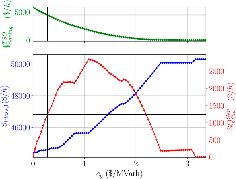
Figure 7. Cost of transmission losses (blue), cost of reactive power support (red), and savings for the TSO (green) plotted over reactive power price.

The price $c_g=1.08\$/MVarh$ leads to the highest value of $\$Q_{\mathit{Cos}}^{\mathit{Gen}}$ and is the best possible option for the GenCos.

An interesting point is $c_g=3.16\$/MVarh$, since it is the first point where $\$Q_{\mathit{Cos}}^{\mathit{Gen}}$ becomes zero again. This marks the first instance where additional reactive power support does not lead to a profit for either the transmission system operator or the generation companies. This is also confirmed when comparing to the savings ${\text{\$}}_{\mathit{Saving}}^{\mathit{TSO}}$ (green) as well as the costs for active power losses $\$P_{\mathit{loss,1}}$ (blue).

Consequently, all prices $(c_g<3.16\$/MVarh)$ benefit the TSO, as improving active losses can compensate for additional reactive power costs. From the point of view of the GenCos, these prices represent additional revenue from reactive power income. Consequently, all prices in the price range $(\mathrm{0,3.16})\$/MVarh$ are valuable for both parties (i.e., all $c_g\in {\mathcal{C}}_g$). The final optimal trade-off of the leader problem, shown as a red star in Figure 6, is illustrated by the intersection point of the two black lines in Figure 7. The best possible trade-off price found for the given scenario is $c_g^{*}=0.28\$/MVarh$.

Figure 8 shows the capability curves of all machines within the study case. The green marker represents the set points $(Q_G^0,P_G^0)$ determined by the resource allocation block, and the blue markers show the newly determined optimal set point for all machines $(Q_G^1,P_G^1)$. As can be seen, the conceptual idea presented is fully realized, and all green and blue dots lie within the boundaries initially introduced in Figure 3. Note that this diagram shows all the constraints of the various machines. Individual constraints are shown as thin lines, whereas limits that are the same for multiple machines are automatically shown as thicker due to their overlap.

Figure 8

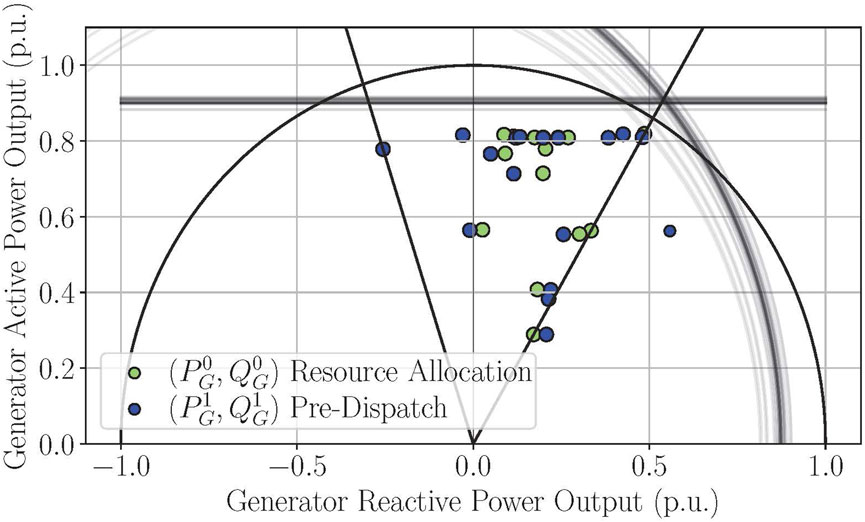
Figure 8. Machine operation points plotted in the various capability curves.

4 Discussion

When considering the follower problem of the pre-dispatch technique and varying the reactive power price $c_g$, which is the decision variable of the leader problem, there is a set of possible prices that are profitable for the TSO and simultaneously lead to extra reactive power income for the GenCos. In the considered study case, this interval was $(\mathrm{0,3.16})\$/MVarh$. Even though the negotiation of the optimizer will lead to additional income for GenCos due to the remuneration of reactive power, it will never lead to an overall profit for GenCos. This is simply because it is a zero-sum game. The savings of the TSO are the total economic losses of the GenCos (i.e., ${\text{\$}}_{\mathit{Saving}}^{\mathit{TSO}}=-{\text{\$}}_{\mathit{Saving}}^{\mathit{GenCos}}$) as written in (Equation 21). Therefore, as soon as the TSO makes savings, the GenCos will gain less than without the pre-dispatch step. However, the pre-dispatch method proposes maximum savings for the TSO while offering the GenCos a fair remuneration for reactive power support.

$\begin{array}{l}{\$}_{\mathit{Saving}}^{\mathit{TSO}}=\mathrm{\Delta }\$P_{\mathrm{0,1}}-\$Q_{\mathit{Cos}}^{\mathit{Gen}}=\left(\$P_{\mathit{loss,0}}-\$P_{\mathit{loss,1}}\right)-c_g^{*}|\mathrm{\Delta }{Q}_{\mathit{Cos}}^{\mathit{Gen}}|=-{\text{\$}}_{\mathit{Saving}}^{\mathit{GenCos}}\hfill \end{array}(21)$

The scenario where ${\text{\$}}_{\mathit{Saving}}^{\mathit{TSO}}=0$ and $\$Q_{\mathit{Cos}}^{\mathit{Gen}}>0$ can theoretically be necessary for calculating the utopia point $z_1$. However, it will never be the final solution, as the leader’s objective is to identify the optimal trade-off between TSO savings and GenCos reactive power incomes.

This discussion briefly addresses the value of $c_g$ at which the maximum of $\$Q_{\mathit{Cos}}^{\mathit{Gen}}$ occurs and which is relevant for determining the utopia point $z_1$, considering the result in Figure 7. When considering the result in Figure 5, it can be seen that $|\mathrm{\Delta }{Q}_{\mathit{Cos}}^{\mathit{Gen}}(c_g)|$ decreases (for almost all points) as $c_g$ increases, which means its derivative is essentially negative. Using the product rule, the derivative of the extra reactive power for GenCos can be written as in Equation 22.

$\frac{\mathrm{d}\$Q_{\mathit{Cos}}^{\mathit{Gen}}\left(c_g\right)}{\mathrm{d}{c}_g}=\underset{0\le }{\underbrace{c_g}}\underset{\le 0}{\underbrace{\frac{\mathrm{d}|\mathrm{\Delta }{Q}_{\mathit{Cos}}^{\mathit{Gen}}\left(c_g\right)|}{\mathrm{d}{c}_g}}}+\underset{0\le }{\underbrace{|\mathrm{\Delta }{Q}_{\mathit{Cos}}^{\mathit{Gen}}\left(c_g\right)|}}(22)$

The derivative $|\mathrm{\Delta }{Q}_{\mathit{Cos}}^{Ge{n}^{\prime }}(c_g)|$ is weighted with a positive price $c_g$. Therefore, for small $c_g$ the large $|\mathrm{\Delta }{Q}_{\mathit{Cos}}^{\mathit{Gen}}(c_g)|$ dominates and leads to a positive $\$Q_{\mathit{Cos}}^{Ge{n}^{\prime }}(c_g)$. The larger $c_g$ becomes, the higher the influence of the negative derivative $|\mathrm{\Delta }{Q}_{\mathit{Cos}}^{Ge{n}^{\prime }}(c_g)|$ and consequently $\$Q_{\mathit{Cos}}^{Ge{n}^{\prime }}(c_g)$ becomes first zero (i.e., it reaches its maximum) and later becomes negative. Therefore, the maximum of $\$Q_{\mathit{Cos}}^{\mathit{Gen}}$ depends significantly on the sensitivity concerning the price $c_g$ and on the function value of $|\mathrm{\Delta }{Q}_{\mathit{Cos}}^{\mathit{Gen}}(c_g)|$.

To solve the formulated bi-level optimization problem, the technique described in Section 2.3 is used. The method is characterized by its simplicity and transparency. However, some points need to be addressed. The variation of the price $c_g$ requires a step size $\delta$ as shown in Figure 4. The choice of this step size is essential because optima may not be found or be imprecise if it is too large. On the other hand, the smaller the chosen $\delta$, the higher the computational cost since, for each price, the OPF in the lower problem has to be computed separately.

One technical aspect that should be considered in future studies is reactive power reserves. These are relevant and have not been taken into account in this paper. If critical contingencies occur, the TSO must ensure that sufficient reserves are available.

The most considerable advantage of the pre-dispatch step is that the TSO can save money by reducing system losses and even financially compensate GenCos fairly.

As mentioned in Section 3, the optimal reactive power price found is $c_g^{*}=0.28\$/MVarh$, which is 0.4 $\%$ of the considered day-ahead price.

According to Wolgast et al. (2022), the value of reactive power is usually less than 1$\%$ of the cost of active power. This estimate is based on the experience with nodal reactive power prices, representing the sensitivity of generation costs calculated in an OPF (Hao and Papalexopoulos, 1997). However, (Hao and Papalexopoulos, 1997) also emphasizes that this price reflects only variable costs. Nevertheless, it is interesting that this article’s optimal price of reactive power is also smaller than 1 $\%$, even though the proposed method does not consider shadow prices.

5 Conclusion

The paper answers the first research question: “What is the reasonable economic value of reactive power when considering active power losses?” as follows: a range of reasonable economic values exists, enabling extra income from reactive power for GenCos and profit for the TSO. Within this price interval $(c_g\in {\mathcal{C}}_g)$, specific prices contribute to objective values along the Pareto front, representing a fair trade-off between the interests of different parties. In the study case examined, the lower limit of this range indicates the optimal outcome for the TSO, which occurs when reactive power is freely available (i.e., $c_g=0\$/MVarh$). Conversely, the upper limit is determined by the maximum additional income GenCos can achieve for reactive power, set at $c_g=1.08\$/MVarh$.

The second research question is: “What is the most equitable price for reactive power that considers all parties involved?” The leader in the bi-level problem described in this article aims to find the best trade-off for GenCos and TSO by choosing the most equitable price for the candidates on the Pareto front. In the considered study case, the price that fulfills all these criteria was $c_g^{*}=0.28\$/MVarh$. It is essential to mention that the price compensates the GenCos for the additional reactive power. Due to the minimization of active power losses, this represents an overall loss for GenCos as they can sell less active power. For the TSO, on the other hand, the solution is profitable. However, the best possible price $c_g$ depends on several factors, including the initial set points, the price sensitivity of $\$Q_{\mathit{Cos}}^{\mathit{Gen}}$, and the prevailing market conditions for that day.

A key contribution of this paper is that the method tries to find a trade-off between the objectives of the GenCos and the TSO. These objectives are in conflict with each other and are formulated as a multiobjective optimization problem in the upper-level problem. Additionally, it provides a transparent procedure for determining the value of reactive power in relation to active power losses.

Reducing active power losses offers considerable benefits to society, as the associated costs are typically passed on to the end-user. The algorithm discussed is not limited to the Nordic grid, but is also relevant in other areas where a similar market design exists.

The challenges and limitations of using the proposed method are related to the solving approach presented, which is simple and easy to understand but requires the user to define a step size of the prices, which has clear disadvantages. However, the efficient solving of the problem was out of the scope of this paper. Another challenge is model accuracy. It is assumed here that the Y-bus matrix of the system is sufficiently precise to perform this type of optimization. In reality, although the TSO has an idea of the model, it cannot be ruled out that there are errors in the model. Since the presented method is model-based, this could lead to calculation errors. The third challenge of this article is the reactive power reserves that, ideally, should be considered to operate the system securely.

All three topics are relevant for further studies. Another relevant topic that is of interest for a future publication is the extent to which shunt-controlled elements of the TSO affect the optimal price $c_g^{*}$. Furthermore, stochastic optimization methods would be interesting to implement in the presented algorithm.

Data availability statement

The raw data supporting the conclusions of this article will be made available by the authors, without undue reservation.

Author contributions

DB: Validation, Investigation, Conceptualization, Software, Writing – review and editing, Visualization, Writing – original draft, Methodology. HR: Writing – review and editing, Writing – original draft, Investigation. SM: Supervision, Project administration, Writing – review and editing, Writing – original draft. TØ: Writing – original draft, Funding acquisition, Project administration, Writing – review and editing. KU: Funding acquisition, Writing – original draft, Conceptualization, Supervision, Writing – review and editing, Methodology.

Funding

The author(s) declare that financial support was received for the research and/or publication of this article. System Optimization between power producer and grid owners (SysOpt), funded by the Research Council of Norway, under project 326673, and the industry partners Statnett, Statkraft, Skagerak Energi, Lede, and AkerSolutions. The funders and partners were involved in the choice of case study.

Conflict of interest

The authors declare that the research was conducted in the absence of any commercial or financial relationships that could be construed as a potential conflict of interest.

Generative AI statement

The author(s) declare that Generative AI was used in the creation of this manuscript. The authors used generative AI (Grammarly by Grammarly Inc. and ChatGPT by OpenAI) to improve the language and clarity of the manuscript. All suggestions were reviewed and revised by the authors.

Any alternative text (alt text) provided alongside figures in this article has been generated by Frontiers with the support of artificial intelligence and reasonable efforts have been made to ensure accuracy, including review by the authors wherever possible. If you identify any issues, please contact us.

Publisher’s note

All claims expressed in this article are solely those of the authors and do not necessarily represent those of their affiliated organizations, or those of the publisher, the editors and the reviewers. Any product that may be evaluated in this article, or claim that may be made by its manufacturer, is not guaranteed or endorsed by the publisher.

References

Almeida, K. C., and Senna, F. S. (2011). Optimal active-reactive power dispatch under competition via bilevel programming. IEEE Trans. Power Syst. 26, 2345–2354. doi:10.1109/TPWRS.2011.2150765

CrossRef Full Text | Google Scholar

Almeida, K., Kocholik, A., and Fernandes, T. (2016). “A bilevel optimal power flow based on fritz-john normalized optimality conditions,” in 2016 Power Systems Computation Conference (PSCC), 1–7. doi:10.1109/PSCC.2016.7540827

CrossRef Full Text | Google Scholar

Baltensperger, D. (2025). Reactive power pre-dispatch. Available online at: https://github.com/baltedan/PreDispatchFinal (Accessed July 24, 2025).

Google Scholar

Bhattacharya, K., and Zhong, J. (2001). Reactive power as an ancillary service. IEEE Trans. Power Syst. 16, 294–300. doi:10.1109/59.918301

CrossRef Full Text | Google Scholar

Cabezas Soldevilla, F. R., and Cabezas Huerta, F. A. (2019). “Minimization of losses in power systems by reactive power dispatch using particle swarm optimization,” in 2019 54th International Universities Power Engineering Conference (UPEC), 1–5. doi:10.1109/UPEC.2019.8893527

CrossRef Full Text | Google Scholar

Conejo, A. J., and Baringo, L. (2018). Power system operations, 11. Springer.

Google Scholar

Davoodi, E., Babaei, E., Mohammadi-Ivatloo, B., and Rasouli, M. (2019). A novel fast semidefinite programming-based approach for optimal reactive power dispatch. IEEE Trans. Industrial Inf. 16, 288–298. doi:10.1109/tii.2019.2918143

CrossRef Full Text | Google Scholar

De, M., and Goswami, S. K. (2014). Optimal reactive power procurement with voltage stability consideration in deregulated power system. IEEE Trans. Power Syst. 29, 2078–2086. doi:10.1109/TPWRS.2014.2308304

CrossRef Full Text | Google Scholar

Eichfelder, G. (2008). Adaptive scalarization methods in multiobjective optimization. Berlin: Springer.

Google Scholar

El-Samahy, I., Bhattacharya, K., Canizares, C., Anjos, M. F., and Pan, J. (2008). A procurement market model for reactive power services considering system security. IEEE Trans. Power Syst. 23, 137–149. doi:10.1109/tpwrs.2007.913296

CrossRef Full Text | Google Scholar

Energinet, F., and Kraftnät, S. (2021). Nordic grid development perspective 2021. Tech. Rep. Nord. Transm. Syst. Oper.

Google Scholar

Feng, D., Cui, B., Chen, T., Niu, L., Wu, Y., Yu, S., et al. (2024). “Solution analysis of optimal reactive power flow considering voltage constraint variation,” in 2024 IEEE PES 16th Asia-Pacific Power and Energy Engineering Conference (Nanjing, China: APPEEC), 1–5. doi:10.1109/APPEEC61255.2024.10922240

CrossRef Full Text | Google Scholar

Hao, S. (2003). A reactive power management proposal for transmission operators. IEEE Trans. Power Syst. 18, 1374–1381. doi:10.1109/TPWRS.2003.818605

CrossRef Full Text | Google Scholar

Hao, S., and Papalexopoulos, A. (1997). Reactive power pricing and management. IEEE Trans. Power Syst. 12, 95–104. doi:10.1109/59.574928

CrossRef Full Text | Google Scholar

Jakobsen, S. H. (2018). Nordic 44 psse version.

Google Scholar

Jiang, M., Guo, Q., Sun, H., and Ge, H. (2022). Leverage reactive power ancillary service under high penetration of renewable energies: an incentive-compatible obligation-based market mechanism. IEEE Trans. Power Syst. 37, 2919–2933. doi:10.1109/TPWRS.2021.3125093

CrossRef Full Text | Google Scholar

Kar, M. K., Kumar, S., Singh, A. K., and Panigrahi, S. (2023). Reactive power management by using a modified differential evolution algorithm. Optim. Control Appl. Methods 44, 967–986. doi:10.1002/oca.2815

CrossRef Full Text | Google Scholar

Kar, M. K., Kanungo, S., Alsaif, F., and Ustun, T. S. (2024). Optimal placement of facts devices using modified whale optimization algorithm for minimization of transmission losses. IEEE Access 12, 130816–130831. doi:10.1109/ACCESS.2024.3458039

CrossRef Full Text | Google Scholar

Kessel, P., and Glavitsch, H. (1986). Estimating the voltage stability of a power system. IEEE Trans. Power Deliv. 1, 346–354. doi:10.1109/TPWRD.1986.4308013

CrossRef Full Text | Google Scholar

Kumar, L., Kar, M. K., and Kumar, S. (2023). Reactive power management of transmission network using evolutionary techniques. J. Electr. Eng. Technol. 18, 123–145. doi:10.1007/s42835-022-01185-1

CrossRef Full Text | Google Scholar

Lamont, J., and Fu, J. (1999). Cost analysis of reactive power support. IEEE Trans. Power Syst. 14, 890–898. doi:10.1109/59.780900

CrossRef Full Text | Google Scholar

Machowski, J., Lubosny, Z., Bialek, J. W., and Bumby, J. R. (2020). Power system dynamics: stability and control. John Wiley & Sons.

Google Scholar

Martín, C. M., Arredondo, F., Arnaltes, S., Alonso-Martínez, J., and Amenedo, J. L. R. (2024). “Optimal re-dispatch and reactive power management in the fuerteventura-lanzarote grid using real-time optimization in the loop,” in 2024 IEEE 15th International Symposium on Power Electronics for Distributed Generation Systems (PEDG), 1–6. doi:10.1109/PEDG61800.2024.10667466

CrossRef Full Text | Google Scholar

Pardalos, P. M., Žilinskas, A., and Žilinskas, J. (2017). Non-convex multi-objective optimization. Springer.

Google Scholar

Rabiee, A., Shayanfar, H. A., and Amjady, N. (2009). Reactive power pricing. IEEE Power & Energy Magazine, january/february.

Google Scholar

Salimin, R. H., Musirin, I., Hamid, Z. A., Aminuddin, N., Zakaria, F., and Senthil Kumar, A. (2024). “Comparative analysis of multi optimization techniques under load variations in optimal reactive power dispatch,” in 2024 IEEE 4th International Conference in Power Engineering Applications (ICPEA), 327–331. doi:10.1109/ICPEA60617.2024.10498487

CrossRef Full Text | Google Scholar

Statnett (2022). NVF 2022: nasjonal veileder for funksjonskrav i kraftsystemet.

Google Scholar

Statnett (2024). Annual and sustainability report 2024. Technical report.

Google Scholar

Transmission, N. G. E. (2019). Annex NGET_A11.11 transmission loss strategy. Technical report. National Grid Electricity Transmission NGET.

Google Scholar

Wolgast, T., Ferenz, S., and Nieße, A. (2022). Reactive power markets: a review. IEEE Access 10, 28397–28410. doi:10.1109/access.2022.3141235

CrossRef Full Text | Google Scholar

Zhang, Y.-j., and Ren, Z.(2005). Optimal reactive power dispatch considering costs of adjusting the control devices. IEEE Trans. Power Syst. 20, 1349–1356. doi:10.1109/TPWRS.2005.851920

CrossRef Full Text | Google Scholar