Two stage coordination planning method of wind power and storage considering uncertainty of distributed source-load

Introduction: With the widespread integration of distributed power sources, the power grid is facing challenges such as increased losses, rising costs, voltage fluctuations, and overload, resulting in greater operational complexity. Traditional scheduling methods are no longer adequate, making reasonable planning of distributed power generation and energy storage configurations particularly crucial.

Methods: This article proposes a two-stage wind-storage coordination planning method that considers source-load uncertainty. The approach is based on an improved antlion algorithm and incorporates distributed energy storage charging and discharging strategies. The first stage focuses on wind power site selection and capacity determination, using voltage offset, network loss, and comprehensive system cost as evaluation indicators. A multi-objective function model is established to balance grid stability and economic efficiency. The second stage introduces distributed energy storage devices to reduce power fluctuations while minimizing the sum of operation, maintenance, and storage investment costs, thereby optimizing the energy storage charging and discharging strategy. The improved antlion algorithm, enhanced with adaptive Lévy flight and golden sine theory, is used to solve the two-stage planning model.

Results: The proposed method effectively improved system-level voltage distribution, reduced network losses, and lowered overall system costs. Specifically, it achieved a 27.95% increase in total capacity, a reduction of 32.14 kW in active power loss, and a total cost decrease of 221,200 yuan. The improved antlion algorithm demonstrated strong search capability, fast convergence speed, and high computational accuracy.

Discussion: The results indicate that the proposed method is better aligned with practical requirements compared to traditional approaches. The improvements in system performance and cost efficiency highlight the effectiveness of the two-stage planning framework and the enhanced optimization algorithm. The method offers a viable solution for the integrated planning of wind power and energy storage systems under uncertainty.

1 Introduction

The integration of distributed power sources injects new voltage power into the distribution network, and the network topology and power flow distribution will also change accordingly. Unreasonable integration may result in problems such as reverse transmission of branch power flow, voltage exceeding limits, and increased line losses, affecting system operation (Fei, 2020). Meanwhile, in distributed power generation, wind and photovoltaic power generation, as the main distributed energy sources, have the advantages of being renewable and environmentally friendly. However, their output power is unstable due to changes in wind speed and light intensity, which may lead to insufficient power supply or resource waste. Therefore, optimizing the configuration of distributed power sources and utilizing energy storage technology to mitigate their adverse effects on the power grid is crucial.

In terms of distributed power generation planning models, Chu and Qiao considered the output efficiency and load rate of distributed power generation units. They formulated a planning model with the objective of minimizing the comprehensive operational cost of the distribution network. Huang et al. calculated power flow and network losses using Monte Carlo sampling and applied a genetic algorithm to optimize costs, network losses, and surplus electricity from distributed power sources. Cao et al. addressed the uncertainties associated with wind, solar, and load variations by employing Latin hypercube sampling combined with an improved synchronous substitution method to generate representative scenarios. The model was solved using an improved particle swarm optimization algorithm, aiming to minimize the annual comprehensive cost. Su et al. proposed a coordinated optimization strategy for wind power, solar power, load demand, and energy storage systems, focusing on determining the optimal power and capacity configuration of energy storage devices. Their objective function included distribution network investment costs, maintenance costs, power purchase costs, and reliability costs, which were optimized using the particle swarm optimization algorithm. Other researchers have also used variables such as network loss as objective functions for analysis and optimization. However, most of the aforementioned studies focus on single-objective optimization, which may overlook the complex interactions in system operations and deviate from practical engineering applications. To address this limitation, scholars both domestically and internationally have conducted further research into multi-objective optimization models. Mohammad et al. constructed a multi-objective function based on indicators such as network loss, voltage deviation, and short-circuit current, and solved it using optimization algorithms. Truong et al. introduced a quasi-adversarial chaotic symbiotic biological search algorithm to address multi-objective optimization problems. Banihashemi et al. developed a multi-objective optimization model aimed at minimizing voltage deviation, line loss, and operational costs, which was solved using an improved genetic algorithm. Li et al. applied the theory of chance-constrained programming and employed the non-dominated sorting genetic algorithm (NSGA) to optimize objectives including minimizing the operational risk of distribution networks and minimizing annual comprehensive costs.

Overall, many literature currently use simple deterministic models to model distributed power generation planning problems, without considering source load uncertainty or the impact of distributed energy storage (Zhenqi, 2021b; Paiva et al., 2017; Ganguly and Samajpati, 2015; Xu et al., 2017; Sivaram et al., 2019; Deyi et al., 2011; Junyang et al., 2018; Chengshan et al., 2006). Therefore, this article will establish a more comprehensive distributed power generation planning model, taking into account the uncertainty of distributed power generation output and the integration of energy storage, to ensure the safety, reliability, and economy of the power system. Therefore, this article proposes a distributed wind storage coordination planning method that takes into account the uncertainty of source load. Firstly, a multi-objective model is established with the constraints of power flow, voltage, and power, aiming to minimize system network losses, voltage deviations, and overall system costs. Taking into account the uncertainty of source and load, a first stage distributed wind power coordination optimization strategy is proposed; Then, taking into account constraints such as power supply, energy storage capacity, and State of charging/discharge, combined with decision variables obtained in the previous stage, a model is established based on system economic indicators, and a second stage distributed energy storage planning method is proposed; Finally, the improved antlion algorithm with adaptive Levy flight and golden sine theory as improvement factors was used to solve the proposed two-stage wind storage coordination planning method. Through simulation verification, it was proved that the proposed method can effectively improve the system voltage distribution level, reduce network losses, and further reduce the overall system cost, bringing good stability and economy to the system operation.

2 Two stage wind storage coordination planning methods

This article considers distributed energy storage charging and discharging strategies and proposes a two-stage wind storage coordination planning method that takes into account source load uncertainty (Chuzhuang, 2017; Weiguo et al., 2016; Zhenqi, 2021a; Haifeng et al., 2016). The specific model diagram is shown in Figure 1.

Figure 1

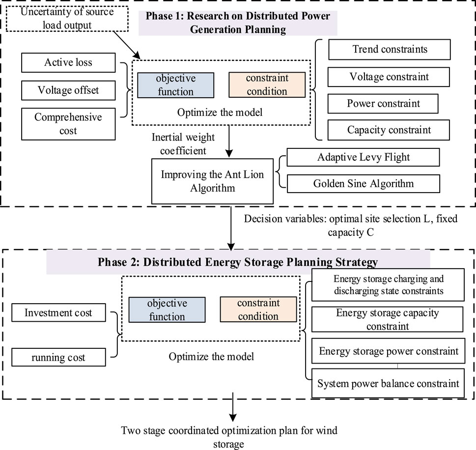
Figure 1. Model diagram of two-stage wind storage coordination planning method.

2.1 Distributed wind power planning model

2.1.1 Objective function

The connection of power supply to the distribution network can effectively improve the system voltage level and reduce network losses, but an unreasonable connection scheme can have a significant impact on the operation of the distribution network and disrupt the safe and reliable operation of the system. Therefore, in this section, a multi-objective system for distribution network operation is established based on three indicators of power grid stability and economy, namely, system network loss, node voltage deviation, and annual comprehensive cost, to coordinate and plan the integration of distributed power sources into the distribution network (Yurong et al., 2020). The specific model is as follows:

$\min f_1=\alpha \frac{f_{loss}}{f_{l\max }}+\beta f_{\Delta U}+\gamma \frac{f_{cb}}{f_{cb\max }}(1)$

In the Formula 1, $f_{loss}$ indicates the active power loss of the system; $f_{\Delta U}$ indicates the system voltage offset value; $f_{cb}$ indicates the comprehensive cost of the system; $f_{l\max }$ indicates the maximum active power loss of the system; $f_{cb\max }$ indicates the maximum comprehensive cost of the system; $\alpha ,\beta ,\gamma$ indicate the inertia weight coefficients of each indicator, determined by the Analytic Hierarchy Process, they are $\alpha =0.6370,\beta =0.0147$, $\gamma =0.2583$。

1. System active power loss $f_{loss}$

$f_{loss}={\displaystyle \sum _{i=1}^L}{G}_{i,j}\left({U_i}^2+{U_j}^2-2U_i{U}_j\cos {\delta }_{ij}\right)(2)$

In the Formula 2, $f_{loss}$ indicates Line loss; $G_{i,j}$ indicates the conductivity value between node i and node j; L indicates the number of system lines; $U_i$, $U_j$ indicate the voltage values of nodes i and j; $\cos {\delta }_{ij}$ indicates the voltage phase angle difference between nodes i and j (Ping et al., 2018).

2. System voltage offset value $f_{\Delta U}$

$f_{\Delta U}={\displaystyle \sum _{j=1}^N}\left|\frac{U_j}{U_n}-1\right|(3)$

In the Formula 3, $f_{\Delta U}$ indicates the voltage offset value; $U_j$ indicates the actual voltage value of the node; $U_n$ indicates the rated voltage of the system; N indicates the number of system nodes.

3. Annual comprehensive cost of the system $f_{cb}$

$f_{cb}={\displaystyle \sum _{s=1}^N}{P}_{\mathrm{L},\mathrm{W}}\left(s\right)\left(f_{yx}^s+f_{tz}^s+f_{loss}^s+f_{ec}^s+f_{gd}^s-f_{bt}^s\right)(4)$

In the Formula 4, N indicates the number of typical scenarios; $P_{\mathrm{L},\mathrm{W}}\left(s\right)$ indicates probability of occurrence of typical wind load scenarios; $f_{\mathrm{yx}}^s$ indicates operating costs in typical scenarios; $f_{\mathrm{tz}}^s$ indicates investment costs in typical scenarios; $f_{loss}^s$ indicates Network loss cost in typical scenarios; $f_{\mathrm{ec}}^s$ indicates Environmental benefits and costs in typical scenarios; $f_{\mathrm{gd}}^s$ indicates under typical scenarios, the cost of purchasing electricity online from a large power company; $f_{\mathrm{bt}}^s$ indicates power generation subsidies in typical scenarios. Among them, the cost expressions are as follows:

a. Running cost:

$f_{yx}=h_f{\displaystyle \sum _{i\in N_f}}{T}_f{P}_{f,i}(5)$

In the Formula 5, $f_{yx}$ indicates operating costs of wind power; $h_f$ indicates the unit cost coefficient for wind power operation is taken as 0.045 yuan per kW hour; $P_{f,i}$ indicates Selected ith wind power generation power; $T_f$ indicates Annual duration of wind power generation; $N_f$ indicates A collection of nodes that can be connected to wind power (Junqiang et al., 2016).

b. Investment cost:

$f_{tz}={\gamma }_f{c}_f{\displaystyle \sum _{i\in N_f}}{P}_{f,i}(6)$

In the Formula 6, $f_{tz}$ indicates Wind power investment cost; ${\gamma }_f$ indicates investment coefficient for wind power, etc.,; $c_f$ indicates unit capacity investment cost of wind power at 10,000 yuan per kW hour; The expression for ${\gamma }_f$ is as follows Formula 7, and in the formula, d indicates annual interest rate which is 0.8, $T_f$ indicates The full life cycle of wind power is taken as 10 years:

${\gamma }_f=\frac{d{\left(1+d\right)}^{T_f}}{d{\left(1+d\right)}^{T_f}-1}(7)$

c. Line loss cost:

$f_s=c_s{\displaystyle \sum _{j=1}^b}{P}_{jl}{T}_{\max }(8)$

In the Formula 8, $c_s$ indicates unit length line loss cost, taken as 0.6 yuan per kW hour; $P_{jl}$ indicates maximum network loss on line j; $T_{\max }$ indicates the maximum annual load loss time is taken as 4200 h.

d. Environmental benefit cost:

$f_{ec}=c_{em}{\displaystyle \sum _{m=1}^n}{\displaystyle \sum _{i\in N_f}}{e}_m\left(P_{load}+P_{loss}-P_{f,i}\right)(9)$

In the Formula 9 n indicates the number of environmental pollutants, $c_{em}$ indicates Unit cost of pollutant m; $e_m$ indicates under the traditional power generation mode, the emission indicators for pollutant m are as follows: sulfur dioxide emission indicator is 4.5 g per kW hour, with a cost of 7.3 yuan per kilogram; nitrogen dioxide emission indicator is 1.64 g per kW hour, with a cost of 10 yuan per kilogram; carbon dioxide emission indicator is 90 g per kW hour, with a cost of 0.8 yuan per kilogram; $P_{load}$ indicates total load of the line; $P_{loss}$ indicates Network loss; all emission indicators are based on typical data of the Chinese power system (China Electricity Council, 2023; Ministry of Ecology and Environment, 2022; Jinnan et al., 2019).

e. Electricity purchase cost:

$f_{gd}=c_{gd}\left(P_{loaad\max }+P_{loss}-{\displaystyle \sum _{i\in N_f}}{T}_f{P}_{f,i}\right)T_1(10)$

In the Formula 10, $c_{gd}$ indicates the unit cost of purchasing electricity is 0.5 yuan per kW hour; $P_{loaad\max }$ indicates maximum system load; $T_1$ indicates the maximum annual load utilization time is taken as 4,200 h.

f. Power generation subsidy:

$f_{bt}=c_{bt}{\displaystyle \sum _{i\in N_f}}{P}_{f,i}(11)$

In the Formula 11, $c_{bt}$ indicates The unit government subsidy fee is 0.4 yuan per kW hour.

2.1.2 Constraint condition

The main constraints considered by the distributed wind power planning model are as follows (Kaiyuan, 2023):

1. Trend constraints

$\left\{\begin{array}{l}\Delta P_i=P_i-U_i{\displaystyle \sum _{j=1}^N}{U}_j\left(G_{ij}\cos {\delta }_{ij}+B_{ij}\sin {\delta }_{ij}\right)=0\\ \Delta Q_i=Q_i-U_i{\displaystyle \sum _{j=1}^N}{U}_j\left(G_{ij}\sin {\delta }_{ij}-B_{ij}\cos {\delta }_{ij}\right)=0\end{array}\right.(12)$

In the Formula 12, $P_i$, $Q_i$ indicate separately active and reactive power of node $i$; $U_i$, $U_j$ indicate separately actual voltage of node j; $G_{ij}$, $B_{ij}$ indicate separately conductance and susceptance of nodes and branches between them; ${\delta }_{ij}$ indicates voltage phase angle difference between nodes; N is the number of system nodes.

2. Node voltage constraint

$U_{i\min }\le U_i\le U_{i\max }(13)$

In the Formula 13, $U_i$ indicates the voltage amplitude of node $i$; $U_{i\min }$, $U_{i\max }$ indicates separately the upper and lower limits of the voltage at node $i$.

3. Branch power constraint

$P_{ij\min }\le P_{ij}\le P_{ij\max }(14)$

In the Formula 14, $P_{ij}$ indicates the active power of the line between nodes $i$ and $j$; $P_{ij\min },P_{ij\max }$ indicates separately the upper and lower limits of active power of the line connecting nodes $i$ and $j$.

4. Wind turbine capacity constraint

$P_{f\min }\le P_f\le P_{f\max }(15)$

In the Formula 15, $P_f$ indicates maximum capacity of wind turbines; $P_{f\max }$ indicates maximum wind power capacity; $P_{f\min }$ indicates minimum capacity of wind power.

2.2 Distributed energy storage planning model

2.2.1 Objective function

In order to further optimize the system operation, this section introduces energy storage devices with peak shaving, valley filling, and flat wave suppression effects (Mohammad, 2014; Truong et al., 2020; Banihashemi et al., 2011; Ke et al., 2017). The reasonable introduction of it greatly improves the stability and performance of the system. However, the cost of energy storage devices is high, and a large amount of investment can also increase the economic operating costs of the system, resulting in resource losses. Therefore, this section focuses on the balance between energy storage devices and power supply and demand, considering energy storage charging and discharging strategies and the entire life cycle of the devices. With the goal of minimizing energy storage investment and operation costs, the optimal energy storage device charging and discharging strategy is obtained. The objective function is as follows (Formula 16) (D et al., 2020):

$\min f_2=f_{ye}+f_{te}(16)$

1. Energy storage operation and maintenance costs $f_{ye}$

$f_{ye}=h_e\left(\int {\eta }_1{s}_c{P}_{ec}-P_{ef}{s}_f/{\eta }_{2}dt\right)(17)$

In the Formula 17, $f_{ye}$ indicates operating costs of energy storage devices; $h_e$ indicates the unit cost coefficient for energy storage operation is set at 0.05 yuan per kW hour; $P_{ec}$, $P_{ef}$ indicate separately Energy storage charging power, energy storage discharging power; ${\eta }_1$, ${\eta }_2$ Indicates the charging and discharging efficiency of the energy storage device, taken as 0.9; $s_c$, $s_f$ indicates the charging and discharging state, with a value of 0 or 1, where 1 represents charging and 0 represents discharging.

2. Energy storage investment cost $f_{tz}$

$f_{te}={\gamma }_e\left[c_{ep}\int P_{e}dt+c_{es}\int S_{e}dt\right](18)$

In the Formula 18, $f_{te}$ indicates investment cost of energy storage devices; ${\gamma }_e$ indicates investment coefficient for energy storage devices, etc. $c_{ep}$, $c_{es}$ indicate separately unit power and capacity cost of energy storage, the energy storage power and capacity are 5,000 yuan per kilowatt or kW hour; $P_e$ indicates actual power of energy storage; $S_e$ indicates energy storage capacity, The expression for ${\gamma }_e$ is as follows (Formula 19), where d indicates an annual interest rate of 0.8, $T_e$ indicates the full life cycle of energy storage and other devices is taken as 10 years:

${\gamma }_e=\frac{d{\left(1+d\right)}^{T_e}}{d{\left(1+d\right)}^{T_e}-1}(19)$

2.2.2 Constraint condition

For the above objective function, the constraints of this model include energy storage device charging and discharging power, capacity constraints, state constraints, as well as system power balance constraints (Ibrahim et al., 2008).

1. Energy storage charging and discharging power constraint

$\left\{\begin{array}{l}{P}_{ec\min }\le P_{ec}\le P_{ec\max }\\ P_{ef\min }\le P_{ef}\le P_{ef\max }\end{array}\right.(20)$

In the Formula 20 $P_{ec}, P_{ef}$ indicate separately energy storage charging and discharging power; $P_{ec\max }, P_{ef\max }$ indicate separately maximum charging and discharging power of energy storage; $P_{ec\min }, P_{ef\min }$ indicate separately minimum charging and discharging power for energy storage.

2. Energy storage capacity constraint

$0\le S_e\le S_{e\max }(21)$

In the Formula 21, $S_e$ indicates capacity of energy storage device; $S_{e\max }$ indicates maximum capacity of energy storage device (Zechun et al., 2017).

3. The constraints on the storage charging and discharging states are shown in Formula 22.

$s_c+s_f=1(22)$

4. System power balance constraint

$P_L+P_{ec}{s}_c=P_f+P_{ef}{s}_f(23)$

In the Formula 23, $P_L$ indicates the power of the load.

3 Solution of two-stage wind storage coordination planning method based on improved antlion algorithm

3.1 Principle of antlion algorithm

The Ant Lion Optimization (ALO) algorithm, proposed by Mirjalili in 2015, is a metaheuristic optimization approach inspired by the hunting behavior of ant lions in nature (Jasim et al., 2023). This algorithm simulates several core processes: random walking, trap building, luring ants, capturing prey, and the implementation of an elite mechanism (Assiri et al., 2020). The key innovation of ALO lies in its adaptive boundary contraction strategy, wherein the radius of the ant lion trap decreases progressively with each iteration. This feature enables a smooth transition from global exploration to local exploitation and helps prevent premature convergence. The algorithm offers advantages such as fewer required parameters and a strong capacity for balance (Abualigah et al., 2020). When applied to solve the two-stage wind-storage coordinated planning method presented in this paper, the specific solution procedure is as follows:

3.1.1 Ant random walk model

$\begin{array}{l}{X_{i,j,t}}^{\prime }=\frac{\left(X_{i,j,t}-\min \left(X_{i,j,t}\right)\right)\times \left(\max {\left(X_{i,j,t}\right)}^t-\min {\left(X_{i,j,t}\right)}^t\right)}{\max \left(X_{i,j,t}\right)-\min \left(X_{i,j,t}\right)}\\ +\min {\left(X_{i,j,t}\right)}^t\end{array}(24)$

In the Formula 24, ${X_{i,j,t}}^{\prime }$ indicates ant random walk normalization route; $X_{i,j,t}$ indicates ants randomly walk along unnormalized routes; $\min \left(X_{i,j,t}\right)$, $\max \left(X_{i,j,t}\right)$ indicate separately the $i$-th ant randomly walks the minimum and maximum values in the $j$-dimensional variable; $\min {\left(X_{i,j,t}\right)}^t$, $\max {\left(X_{i,j,t}\right)}^t$ indicate the $i$-th ant randomly walks to the minimum and maximum values after the $j$-dimensional variable iteration.

3.1.2 Antlion trap model

Simulate the process using the roulette wheel selection mechanism and define it as:

$\left\{\begin{array}{l}\min {\left(X_{i,j,t}\right)}^t=A{L_j}^t+\min {\left(X\right)}^t\\ \max {\left(X_{i,j,t}\right)}^t=A{L_j}^t+\max {\left(X\right)}^t\end{array}\right.(25)$

In the Formula 25, $A{L_j}^t$ indicates the position of the jth antlion in the $t$-th iteration; $\min {\left(X\right)}^t$, $\max {\left(X\right)}^t$ indicate separately the minimum and maximum values of all ants after the $t$-th iteration.

3.1.3 Ant trapped in trap model

The trap range is defined as follows (Formula 26):

$\left\{\begin{array}{l}{\left[\max {\left(X\right)}^t\right]}^{\prime }=\frac{\max {\left(X\right)}^t}{I}\\ {\left[\min {\left(X\right)}^t\right]}^{\prime }=\frac{\min {\left(X\right)}^t}{I}\end{array}\right.(26)$

$I=\frac{{10}^{w}t}{T}(27)$

In the Formula 27, I indicates the size of the trap range; $w$ indicates the calibration coefficient is related to the number of iterations; $T$ indicates maximum number of iterations.

3.1.4 Elite antlion model

The antlion with the highest fitness during each iteration is called the elite antlion, In the $t$ iteration, the position of the $i$ ant is:

$A_i^t=\frac{P_{AL}^t+P_{ALE}^t}{2}(28)$

In the Formula 28, $A_i^t$ indicates the position of the ith ant in the $t$-th iteration; $P_{AL}^t$, $P_{ALE}^t$ indicate separately the step size of ants randomly walking around the antlion and elite antlion in the $t$-th iteration; (5) Antlions prey on ants and reconstruct new trap models

When the fitness of ants is higher than that of antlions, ants are captured. At this point, the antlion sets the capture location as the reconstruction trap location. The formula for this model is:

$A{L}_j^t=A_i^{t}iff\left(A_i^t\right)>f\left(A{L}_j^t\right)(29)$

In the Formula 29, $A_i^t$ indicates the position of the $i$-th ant in the $t$-th iteration; $A{L}_j^t$ indicates the position of the $j$-th antlion in the $t$-th iteration.

3.2 Improvement of antlion algorithm

Actual tests demonstrate that although the traditional ant lion algorithm employs a diversified search strategy, it suffers from limited local search capability and is prone to becoming trapped in local optima, thereby constraining improvements in solution quality. Furthermore, conventional algorithms exhibit inadequate convergence accuracy in high-precision application scenarios. To address these limitations, this study proposes an adaptive Levy flight mechanism. Leveraging its long-step-length jumping characteristic, this mechanism effectively enables individuals to escape local optimal regions, thereby enhancing the algorithm’s global exploration capability and mitigating premature convergence. Additionally, the golden sine theory is incorporated. Utilizing its refined search and rapid convergence properties, this approach facilitates more precise and efficient local exploitation within promising solution regions, significantly improving the algorithm’s convergence accuracy. By integrating an adaptive strategy that dynamically adjusts the balance between Levy flight-based exploration and golden sine-based exploitation, the proposed method intelligently coordinates global search and local development processes, ensuring high-precision convergence while effectively avoiding local optima (Jianfang et al., 2025).

3.2.1 Adaptive levy flight (Tanyildizi and Demir, 2017)

The random walk pattern of Levi’s flight follows the Levi distribution shown in Equation 30:

$P_{a,b}\left(x\right)=\frac{1}{\pi }{\int }_0^x\exp \left(m{n}^a\right)\cos \left(qz\right)dn(30)$

In the Formula 30, a represents the peak height of the Levi distribution. When a is a non integer positive real number, the position update is performed using the method shown in Formula 31 below:

$A_i^{t+1}=A_i^t+a·\text{Levy}\left(\theta \right)(31)$

In the Formula 31, $A_i^t$, $A_i^{t+1}$ indicate the position of the $i$-th ant in the $t$-th and $t$ +1st iterations; $\text{Levy}\left(\theta \right)$ indicates a random search path that follows the Levy distribution. $\text{Levy}\left(\theta \right)$ conforms to the following constraints:

$\text{Levy}\left(\theta \right)\sim \frac{\phi u}{\mid v{\mid }^{1/2}}(32)$

In the Formula 32, $\theta$ indicates levy parameter, usually setting at 1.5; μ and ν indicate random numbers that follow a standard normal distribution; The expression for $\phi$ is as follows (Formula 33):

$\phi ={\left[\frac{\mathrm{\Gamma }\left(1+\theta \right)\sin \left(\pi \theta /2\right)}{\mathrm{\Gamma }\left[\left(1+\theta \right)/2\right]\theta 2^{\left(\theta -1\right)/2}}\right]}^{1/\theta }(33)$

In this section, an adaptive Levy flight mechanism is introduced to mutate ants in their position updates, making their updated positions more diverse. The introduction of this improvement factor makes the search scope more comprehensive, the overall optimization efficiency of the population higher, and effectively avoids the solution results from falling into local optima.

3.2.2 Golden sine algorithm (Ghaemi et al., 2009)

The position update process of the Golden Sine Algorithm is shown in the following Formula 34:

$X_i^{T+1}=X_i^T\mid \sin \left(R_1\right)\mid +R_2\sin \left(R_1\right)\mid x_1{P}_i^T-x_2{X}_i^T\mid (34)$

During the position update process, $s$ individual positions are randomly generated first, and $X_i^T=\left\{X_{i1},X_{i2},X_{i3},······,X_{in}\right\}$ is used to represent the position of the $i$-th particle in the Tth iteration in $n$-dimensional space, among them $i=1,2,\cdots ,s$, Use $P_i^T=\left\{P_{i1},P_{i1},P_{i1},......,P_{in}\right\}$ to represent the historical best position of the $i$-th particle in the Tth iteration. $R_1$ and $R_2$ are random number, $R_1\in \left[0,2\pi \right]$, $R_2\in \left[0,\pi \right]$. $x_1$ and $x_2$ are coefficients obtained through the golden ratios, and golden ratios are $\tau =\left(\sqrt{5}-1\right)/2$, $x_1=-\pi +2\pi \left(1-\tau \right)$, $x_2=-\pi +2\pi \tau$.

The steps of the improved antlion algorithm based on adaptive Levy flight and golden sine algorithm are shown in Figure 2:

Figure 2

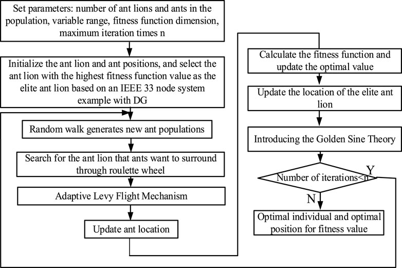
Figure 2. Improved antlion algorithm solution flow chart.

4 Example analysis

4.1 Validation of the superiority of the improved antlion algorithm

Based on the objective function and corresponding constraints mentioned in Section 2, this section adopts the antlion algorithm, improved antlion algorithm, and particle swarm algorithm for optimization and solution. The number of iterations for each algorithm mentioned above is set to 100, with a population size of 40. This example uses the MATLAB 2021a simulation platform, with a computer model of Thinkpad X13, a processor model of Intel (R) Core (TM) i5-10210U CPU @ 1.60 GHz, and a memory capacity of 8 GB. The resulting running results are shown in the following figure (Zhou et al., 2024).

From the comparative analysis of Figure 3, it can be seen that compared to the other two algorithms, the improved Antlion algorithm has a longer computation time due to the addition of adaptive Levy flight and golden sine algorithm modules. The initial iteration curves of the three algorithms all approximate a linear descent, indicating that all three algorithms have fast optimization speeds in the initial stage. However, after multiple iterations, the convergence speed of particle swarm optimization algorithm and antlion algorithm is significantly slower than that of the improved antlion algorithm. The improved antlion algorithm obtained the optimal solution in the 18th iteration, the antlion algorithm obtained the optimal solution in the 44th iteration, and the particle swarm optimization algorithm obtained the optimal solution in the 56th iteration. Therefore, it can be seen that the introduction of the improvement factor in the improved antlion algorithm accelerates its convergence speed, enhances its optimization ability, and correspondingly increases its convergence accuracy. Therefore, it can be verified that the improved antlion algorithm used in this article has the advantages of strong search ability, fast convergence speed, and high accuracy in dealing with distributed power planning problems.

Figure 3

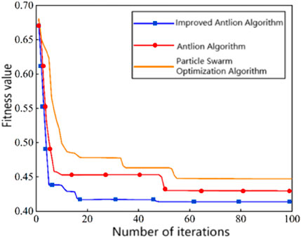
Figure 3. Variation of fitness values of four intelligent optimization algorithms with iteration times.

4.2 Example parameter settings

This section refers to the IEEE 33 node standard distribution network model, and the power flow calculation adopts the forward backward method. The system consists of 33 nodes, 32 branches, a reference voltage level of 12.66KV, a three-phase reference power value of 10MVA, and a balance node that is not connected to distributed power sources. The total load size of the system is 3,715 + j2300KVA, with nodes 1–8 and 17–26 selected for industrial load, and the total load size is 2,150 + j1045KVA; The residential load is taken from nodes 9–16 and 27–33, with a total load size of 1,565 + j1255KVA. Typical wind load scenarios are generated using the couple function and k-means clustering method, as shown in Figure 4.

Figure 4

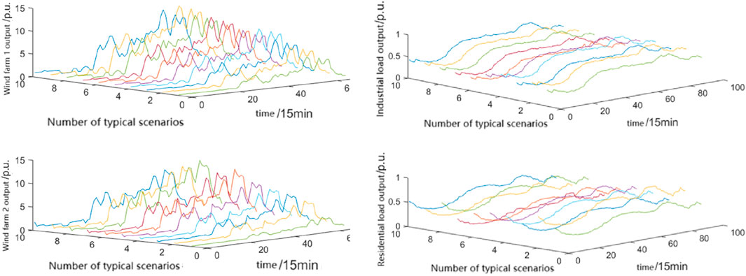
Figure 4. Typical scenario of wind farm output.

The probabilities of each scenario are shown in Figures 5, 6, and the typical wind load scenario is taken as 10 for solving wind power planning.

Figure 5

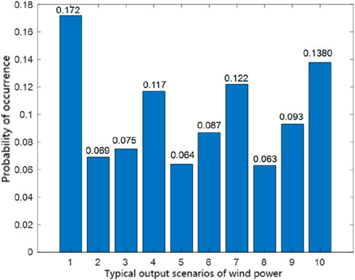
Figure 5. Probability of typical output scenarios of coupled wind power.

Figure 6

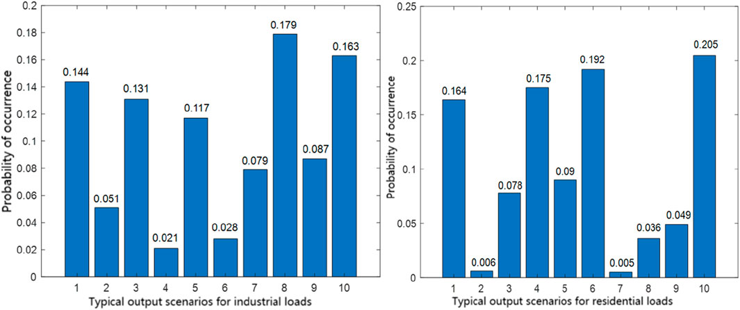
Figure 6. Probability of typical load output scenarios.

4.3 Phase 1 distributed wind power planning and solution

Based on the above distribution network model and the output probability of the source load scenario, this section adopts the improved antlion algorithm mentioned in Section 2.2, selects 40 individual antlions, and performs optimization operations with a maximum iteration of 100 times. To verify the effectiveness of the proposed method, this section introduces three additional planning methods for comparative analysis. The results of the four solutions are shown in Table 1 and Figure 7.

Table 1

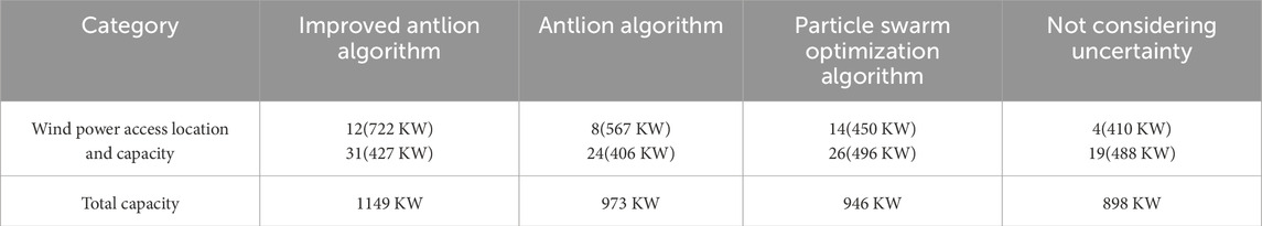
Table 1. Power planning methods under different methods.

Figure 7

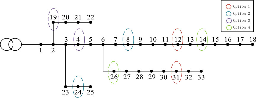
Figure 7. IEEE33 node distribution network.

Compared with the other three schemes, the planning method solved by the improved antlion algorithm has the highest power access capacity and penetration rate, laying a good foundation for the economic and reliable operation of the system. To further verify the effectiveness of the method proposed in this article, this section will analyze it one by one from three aspects: voltage distribution, active power loss and voltage deviation, and system comprehensive cost.

4.3.1 System voltage distribution

Figure 8 shows the system voltage distribution diagrams corresponding to the four schemes. As shown in the figure, the improved antlion algorithm results in the most significant voltage increase effect, further verifying the superiority of the planning method based on the improved antlion algorithm.

Figure 8

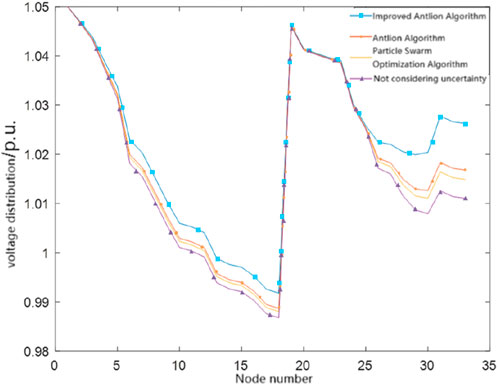
Figure 8. Voltage distribution diagram of different schemes.

4.3.2 System active power loss and voltage deviation

The active losses and voltage deviations of each scheme are shown in Table 2. From the table, it can be seen that the improved antlion algorithm has the smallest active power loss and voltage deviation compared to the other three schemes, which can effectively improve the economy and stability of power system operation compared to other schemes。

Table 2

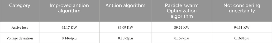
Table 2. Active loss and voltage deviation.

4.3.3 System comprehensive cost

The system cost diagrams for different schemes are shown in Figure 9:

Figure 9

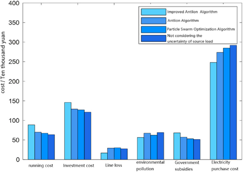
Figure 9. System cost chart for different solutions.

The improved antlion algorithm planning method has the highest power supply capacity and penetration rate, resulting in higher power investment and operating costs compared to other schemes. However, due to the reasonable planning of this scheme, the system line losses, environmental pollution, and power purchase costs are significantly reduced, effectively offsetting the high investment and operation costs. Table 3 shows the comparison of comprehensive costs under different schemes.

Table 3

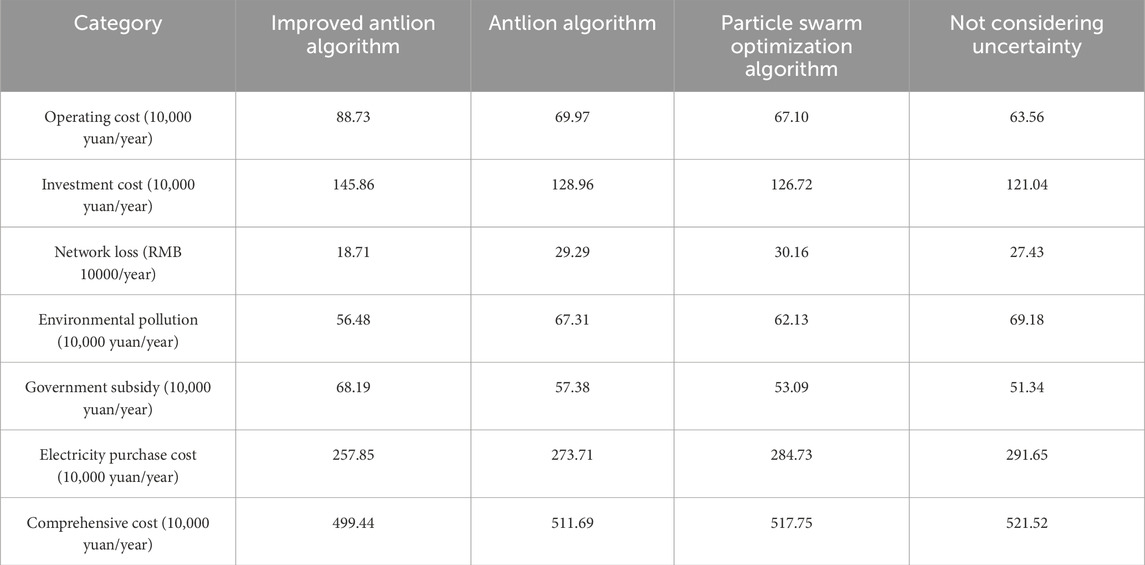
Table 3. Comprehensive costs under different schemes.

The cost of line loss for improving the antlion algorithm planning method is 187,100 yuan, which is the smallest compared to the other three schemes. This indicates that the proposed improved antlion algorithm can effectively assist distributed power generation in reducing line network loss and improving the system’s economic efficiency. In terms of purchasing electricity costs, due to the integration of distributed power sources, the self supply level of the system has increased, and the demand for purchasing electricity from the power grid has correspondingly decreased, thereby reducing the cost of purchasing electricity. Compared with the other three schemes, the introduction of the improved antlion algorithm further reduces the system’s electricity purchase cost, verifying the superiority of this algorithm.

4.4 Phase 2 distributed energy storage planning and solution

Based on the planning model described in Section 1, combined with the improved Antlion algorithm, the following energy storage charging and discharging and configuration planning strategies can be obtained. Table 4 and Figure 10 show the layout results of the energy storage device.

Table 4

Table 4. Distributed energy storage configuration schemes under different methods.

Figure 10

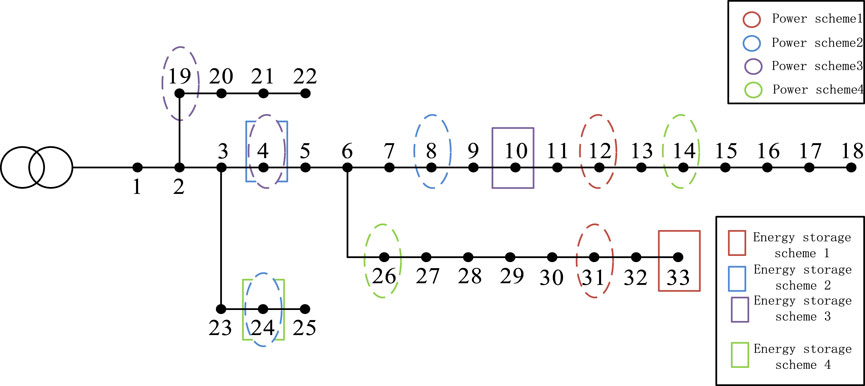
Figure 10. Wind storage coordination optimization model.

According to the particle swarm algorithm and planning methods that do not consider source load uncertainty, the energy storage installation capacity is relatively small. In the solution based on the antlion algorithm, although the energy storage access capacity is large, due to the proximity of the 4 nodes to the front end of the line and the higher economic cost of large energy storage capacity, the antlion algorithm solution is not suitable as the optimal processing method compared to the improved antlion algorithm. The introduction of improved antlion algorithm makes the energy storage installation capacity moderate, with good economic benefits, and the installation location close to distributed power sources, which is in line with the original intention of energy storage installation, that is, to suppress real-time power fluctuations caused by the integration of distributed power sources.

Figure 11 shows the charging and discharging status of energy storage and the charging and discharging power situation. It can be seen from the figure that energy storage is not always working, but indirectly charging and discharging based on the real-time operating status of the system. In order to verify the effectiveness of energy storage access, this section selects typical days as shown in Figure 12 for validity verification.

Figure 11

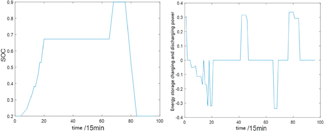
Figure 11. State of charging/discharge and power.

Figure 12

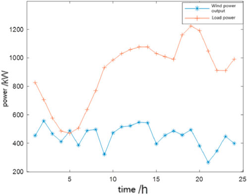
Figure 12. Typical daily wind load output.

As shown in Figure 13, with the addition of distributed energy storage devices, the load curve fluctuation of the system on typical days shows a significant easing trend compared to before the addition of energy storage devices, and the peak valley difference of load output is significantly reduced, suppressing power fluctuations.

Figure 13

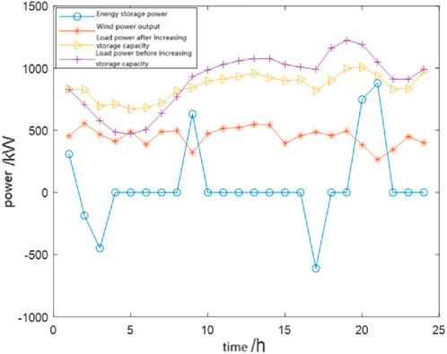
Figure 13. System power before and after energy storage addition.

Based on the energy storage charging and discharging strategy in Figure 11, it can be seen that during peak load operation, the energy storage device serves as a power source to assist distributed wind power in providing electricity to the system. However, during low load periods, the energy storage device acts as a load and plays a charging role. The integration of distributed energy storage devices is coordinated with distributed wind power generation. When wind power output is low, energy storage serves as a power source to supply power to the load, achieving reliable operation of the system.

5 Summary

This article introduces a distributed energy storage charging and discharging strategy, and proposes a two-stage wind storage coordination planning method, which is solved by an improved antlion algorithm. The main conclusions are as follows: (1) The improved antlion algorithm with adaptive Levy flight and golden sine algorithm can effectively improve the voltage distribution level of the system, reduce network losses, and further reduce the overall cost of the system, bringing good stability and economy to the system operation. (2) The integration of distributed energy storage effectively suppresses power fluctuations caused by the uncertainty of distributed power generation output, and cooperates with distributed wind power to provide power supply. Although the cost of the method proposed in this paper is not optimal, it combines economy and reliability, providing decision-makers with more diverse and reasonable planning methods to choose from.

This study is subject to certain limitations. First, the cost-benefit trade-off of the proposed method in specific application scenarios needs to be more accurately quantified. Second, the algorithm’s solution efficiency and its application potential in large-scale systems require further in-depth validation. Future research will focus on the coordinated planning of wind power and energy storage systems, incorporating multi-time-scale and multi-type flexible resources. Additionally, the adaptability of the planning framework to uncertainties and extreme operating conditions will be enhanced.

Data availability statement

The raw data supporting the conclusions of this article will be made available by the authors, without undue reservation.

Author contributions

SS: Funding acquisition, Resources, Writing – original draft, Writing – review and editing, Project administration, Validation, Conceptualization, Methodology, Supervision. JZ: Data curation, Formal Analysis, Conceptualization, Writing – review and editing, Writing – original draft. QX: Formal Analysis, Investigation, Writing – original draft. LS: Visualization, Writing – review and editing, Validation, Supervision. CW: Methodology, Software, Writing – review and editing. SX: Data curation, Formal Analysis, Writing – review and editing. MD: Methodology, Writing – review and editing, Software.

Funding

The author(s) declare that financial support was received for the research and/or publication of this article. This work was supported by the Science and Technology Project of China Yunnan Power Grid Corporation (YPGC) (Project Number: YNKJXM20222105).

Conflict of interest

Authors SS and QX were employed by Electric Power Research institute of Yunnan Electric Power Grid Co. Ltd.

The remaining authors declare that the research was conducted in the absence of any commercial or financial relationships that could be construed as a potential conflict of interest.

The authors declare that this study received funding from China Yunnan Power Grid Corporation. The funder had the following involvement in the study: High proportion clean energy county multi energy collaborative distribution system operation control and resilience enhancement technology.

Generative AI statement

The author(s) declare that no Generative AI was used in the creation of this manuscript.

Any alternative text (alt text) provided alongside figures in this article has been generated by Frontiers with the support of artificial intelligence and reasonable efforts have been made to ensure accuracy, including review by the authors wherever possible. If you identify any issues, please contact us.

Publisher’s note

All claims expressed in this article are solely those of the authors and do not necessarily represent those of their affiliated organizations, or those of the publisher, the editors and the reviewers. Any product that may be evaluated in this article, or claim that may be made by its manufacturer, is not guaranteed or endorsed by the publisher.

References

Abualigah, L., Shehab, M., Alshinwan, M., Mirjalili, S., and Elaziz, M. A. (2020). Ant lion optimizer: a comprehensive survey of its variants and applications. Archives Comput. Methods Eng. 28 (3), 1397–1416. doi:10.1007/s11831-020-09420-6

CrossRef Full Text | Google Scholar

Assiri, A. S., Hussien, A. G., and Amin, M. (2020). Ant lion optimization: variants, hybrids, and applications. IEEE Access 8, 77746–77764. doi:10.1109/access.2020.2990338

CrossRef Full Text | Google Scholar

Banihashemi, F., Lesani, H., and Makhzani, A. S. (2011). Locating and capacity determination of distributed generations using none-dominated sorting genetic algorithm international conference in swarm intelligence. Springer, 211–298.

Google Scholar

Chengshan, W., Kai, C., and Yinghua, X. (2006). Location and capacity determination of distributed power sources in distribution network expansion planning. Power Syst. Autom. 03, 38–43.

Google Scholar

China Electricity Council (2023). “China's electricity industry annual development report,”. Beijing: China Building Materials Industry Press, 56–59.

Google Scholar

Chuzhuang, Q. (2017). Fuquan distributed wind power source site selection and capacity determination considering wind power and load timing. J. Power Syst. Automation 29 (10), 85–90.

Google Scholar

Ding, Q., Zeng, P., and Sun, Y. (2020). A planning method for the placement and sizing of distributed energy storage system considering the uncertainty of renewable energy sources. Energy Storage Sci. Technol. 9 (1), 162.

Google Scholar

Deyi, Y., Zhengyou, H., and Tianlei, Z. (2011). Distributed power generation site selection and capacity determination based on adaptive mutation particle swarm algorithm. Power Grid Technol. 35 (06), 155–160. doi:10.13335/j.1000-3673.pst.2011.06.032

CrossRef Full Text | Google Scholar

Fei, M. (2020). Analysis of the influence of the development of distributed power on the existing power grid. Int. J. Soc. Sci. Univ. 3 (2), 98–105.

Google Scholar

Ganguly, S., and Samajpati, D. (2015). Distributed generation allocation on radial distribution networks under uncertainties of load and generation using genetic algorithm. IEEE Trans. Sustain. Energy 6 (3), 688–697. doi:10.1109/tste.2015.2406915

CrossRef Full Text | Google Scholar

Ghaemi, M., Zabihinpour, Z., and Asgari, Y. (2009). Computer simulation study of the levy flight process. Physicia A Stat. Mech. Its Appl. 388 (8), 1509–1514. doi:10.1016/j.physa.2008.12.071

CrossRef Full Text | Google Scholar

Haifeng, S., Mengjin, H., and Zhirui, L. (2016). Distributed power generation planning with energy storage devices based on temporal characteristics power automation equipment. 36 (06) 56–63.

Google Scholar

Ibrahim, H., Ilinca, A., and Perron, J. (2008). Energy storage systems—Characteristics and comparisons. Renew. Sustain. Energy Rev. 12 (5), 1221–1250. doi:10.1016/j.rser.2007.01.023

CrossRef Full Text | Google Scholar

Jasim, A. M., Jasim, B. H., Baiceanu, F. C., and Neagu, B. C. (2023). Optimized sizing of energy management system for off-grid hybrid solar/wind/battery/biogasifier/diesel microgrid system. Mathematics 11 (5), 1248. doi:10.3390/math11051248

CrossRef Full Text | Google Scholar

Jianfang, Y., Sheng, L., Junjie, W., and Xiaoyi, L. (2025). Ant lion optimization algorithm integrating levy flight and golden sine. Comput. Appl. Res., 2349–2353.

Google Scholar

Jinnan, W., Hongqiang, J., and Fang. Methods, Y. (2019). Research on environmental pollution cost assessment in China. China Environ. Sci. 39 (5), 2229–2238.

Google Scholar

Junqiang, W., Bo, Z., and Jianhua, Z. (2016). Adjustable robust optimization for distributed wind power planning in distribution network. Power Syst. Technol. 40 (7), 1989–1995.

Google Scholar

Junyang, M., Tao, M., and Hang, Y. (2018). Distributed wind power source location and capacity determination in distribution network based on improved genetic algorithm. Electr. Autom. 40 (06), 38–41.

Google Scholar

Kaiyuan, X. U. (2023). Experience summary on general arrangement of distributed wind power project. Eng. Technol. Res. 6 (5), 115–118.

Google Scholar

Ke, L., Nengling, T., and Shenxi, Z. (2017). Multi objective planning method for distributed power generation considering correlation. Power Syst. Autom. 41 (09), 51–57.

Google Scholar

Ministry of Ecology and Environment. (2022). Announcement of carbon dioxide emission factors for provincial power grids in China [EB/OL].

Google Scholar

Mohammad, H. (2014). “Moradi, S.M. reza Tousi,Mohammad abedini,” in Multi-objective PFDE algorithm for solving the optimal siting and sizing problem of multiple DG sources. Elsevier Ltd, 56.

Google Scholar

Paiva, F., Costa, J., and Silva, C. (2017). A serendipity-based approach to enhance particle swarm optimization using scout particles. IEEE Lat. Am. Trans. 15 (6), 1101–1112. doi:10.1109/tla.2017.7932698

CrossRef Full Text | Google Scholar

Ping, J., Tiejiang, Y., and Yong, C. (2018). Study on capacity planning of distributed wind-storage integration system. Power Capacitor and React. Power Compens. 39 (1), 135–141.

Google Scholar

Sivaram, M., Batri, K., and Amin Salih, M. (2019). Exploiting the local optima in genetic algorithm using tabu search. Indian J. Sci. Technol. 1, 1–13. doi:10.17485/ijst/2019/v12i1/139577

CrossRef Full Text | Google Scholar

Tanyildizi, E., and Demir, G. (2017). Golden sine algorithm: a novel math-inspired algorithm. Adv. Electr. and Comput. Eng. 17 (2), 71–78. doi:10.4316/aece.2017.02010

CrossRef Full Text | Google Scholar

Truong, K. H., Nallagownden, P., Elamvazuthi, I., and Vo, D. N. (2020). Aquasi-oppositional-chaotic symbiotic organisms search algorithm for optimal allocation of DG in radial distribution networks. Appl. Soft Comput. 88, 106067. doi:10.1016/j.asoc.2020.106067

CrossRef Full Text | Google Scholar

Weiguo, H., Junyong, L., and Zhenbo, W. (2016). Distributed power generation site selection and capacity determination considering redundant power and timing high voltage electrical appliances. 52 (03), 93–99.

Google Scholar

Xu, M., Li, S., and Guo, J. (2017). Optimization of multiple traveling salesman problem based on simulated annealing genetic algorithm. ed. MATEC Web Conf. EDP Sci. 100, 02025. doi:10.1051/matecconf/201710002025

CrossRef Full Text | Google Scholar

Yurong, W., Ruolin, Y., and Sixuan, X. (2020). Capacity planning of distributed wind power based on a variable-structure copula involving energy storage systems. Energies 13 (7), 3450. doi:10.3390/en13143602

CrossRef Full Text | Google Scholar

Zechun, H., Yonghua, S., and Zhiwei, X. (2017). Multi-objective optimization planning of large-scale distributed energy storage in distribution networks. Proc. CSEE 37 (1), 82–91.

Google Scholar

Zhenqi, C. (2021a). Peng minfang, shen Mei'e distributed power generation site selection and capacity determination considering source load uncertainty. J. Power Syst. Automation 33 (02), 59–65.

Google Scholar

Zhenqi, C. (2021b). Site selection and capacity determination of wind and solar energy storage based on two-stage coordinated optimization Hunan university.

Google Scholar

Zhou, M., Ma, F., and Jin, W. (2024). Long-term cost planning of data-driven wind-storage hybrid systems. Renew. Energy 223, 120073–120082. doi:10.1016/j.renene.2024.120073

CrossRef Full Text | Google Scholar