Research on improved cable-length-adaptive sensorless vector control for drives of induction motors in deep-sea oilfields

Introduction: This paper addresses the issue of the insufficient adaptability of existing vector control algorithms to filter and compensate for long cable parameters (under the influence of parasitic impedance, parasitic capacitive reactance, and parasitic inductive reactance), which leads to unresolved stability and harmonic issues in long-cable drives for deep-sea oil fields.

Methods: By establishing the complete system transfer function of filter-cable-motor, providing the Lyapunov proof of asymptotic stability, a sensorless vector control algorithm based on Lyapunov theory was proposed. This paper also quantified the analysis of variations in long cable parameters over time in the deep-sea environment and incorporated it into the proposed long cable model. A Lyapunov function was constructed. For further analysis of the stability of the proposed function, the long cable health model was introduced and verified. Simulations were conducted under various frequencies, work situations, and with the introduction of time-sensitivity parameters for long cables. The improved algorithm demonstrates certain adaptability to time-sensitivity parameters and improves the torque and current response of the induction motor.

Results: Experimental verifications on no-load startup, sudden load, and sudden unload were carried out. The Fast Fourier Transform (FFT) simulation results demonstrate that during 10 Hz no-load operation, the Total Harmonic Distortion (THD) decreases from 8.28% to 5.41%; during 30 Hz no-load operation, it decreases from 7.70% to 4.45%; while during 50 Hz no-load operation, it drops from 4.41% to 4.37%. The THD at 10 Hz, 30 Hz, and 50 Hz frequencies drops by 2.87%, 3.35%, and 0.04% respectively.

Discussion: Future work will focus on applications in deep-sea oil extraction and on further improving the simulations and experiments.

1 Introduction

1.1 Background of the deep-sea oilfield extraction

Induction motors are widely used in various industrial scenarios, which are crucial equipment for deep-sea oil extraction (Xia et al., 2018; Chien and Bucknall, 2007; Liang et al., 2015), as they enhance the efficiency and output of oil production. A majority of extracted oil is obtained through induction motors (Yao, 2002; Bonczar, 2022; Avery, 2023), which are cost-effective, stable, and reliable. These devices typically require variable frequency drives (VFDs) for operation (Rahman and Salim, 2019; Singh and Naikan, 2018; Sprovieri, 2014; Callegari et al., 2023). During extraction, induction motors are usually installed at the base of deep-sea oil platforms.

VFDs, commonly composed of IGBTs (three-phase or two-phase), are controllable devices that offer stability, closed-loop operation, and adaptability to various control algorithms based on operational requirements. Consequently, VFDs are widely utilized in induction motor control.

To control VFDs, achieve inversion to supply power to an induction motor, vector control algorithms, direct torque control algorithms, and control algorithms that use the sliding mode observer can be employed. The vector control algorithm, as a widely used control method, exhibits excellent characteristics for controlling induction motor (Yaseen and Al-Khazraji, 2025; Hasan, 2025; Das and Chatterjee, 2025). Its features are effective, direct control, and stable performance. Due to the traditional vector control algorithm not being able to directly measure the three-phase voltage and three-phase current of the induction motor when long cables are added (Smochek et al., 2016; Liang et al., 2014), the stability decreases. Traditional vector control may have the problem of inaccurate estimation of rotor flux linkage (Lekhchine et al., 2014), and may exhibit higher harmonic distortion and poor motor starting performance under conditions of a long cable.

1.2 Previous studies and the research content of this paper

1.2.1 Previous research and comparison with this paper

The previous research (Deng. et al., 2019), as shown in Table 1, a π model for long cables was established for the first time, which compensates for voltage and current deviations through coordinate transformation, thereby improving the starting torque. The simulation and experiment of 50 Hz no-load and sudden load start-up are carried out. There is no quantitative analysis of the THD metric and no stability proof. Specifically, it didn’t add the function to the system’s transfer function, didn’t prove its stability, didn’t analyze the parameters of the long cable that introduces time sensitivity, and didn't perform any field test and verification under actual deep-sea conditions.

Table 1

Table 1. Comparison with previous studies.

Reference (Tao et al., 2024) proposed a novel super-twisting algorithm-based sliding mode observer for the multi-vector model-free predictive control (STASMO-MVMPC) method, applied to permanent magnet synchronous motors, which improved control performance. Reference (Liu et al., 2025) by reducing the number of voltage vectors and calculating the operating time of each level based on volt-second balance, the voltage balance issue of the inverter is resolved, offering the advantages of simplicity and low loss. Reference (Zhu et al., 2024) proposes an improved decoupling control method combining the grey wolf optimization algorithm and LSSVM, with mathematical model derivation conducted. The proposed algorithm demonstrates superior performance. Reference (Qiao et al., 2025) proposes a multi-vector direct model predictive torque control algorithm, which optimizes the issue of difficulty in guaranteeing the optimal characteristics of voltage vectors. Comparisons with recent control strategies demonstrate its excellent stability and dynamic response. Reference (Dursun, 2023) proposed a Runge-Kutta (RK) algorithm, featuring a robust mathematical structure, that addresses the high-dimensional issues of asynchronous motors by employing control algorithms such as FDB-RK, RK, etc. Reference (Adamczyk and Orlowska-Kowalska, 2024) established an observer-based vector control algorithm for induction motor control. Reference (Boukhili et al., 2022) proposes a current sensing disturbance control algorithm to address the critical importance of current in vector control, requiring a method to detect current loss. The proposed control algorithm demonstrates effective detection performance and improves motor and generator performance. Reference (Feng et al., 2024) to address the issue of reduced accuracy in LIM speed identification caused by system disturbances, a speed observation method based on the Coleman filter is proposed, which enhances the effectiveness of the LIM algorithm. Reference (Qin et al., 2015) introduced an improved PID controller aimed at enhancing acceleration performance, and its effectiveness was verified through comparisons with other controllers. As shown in Table 1, recent studies (Tao et al., 2024) have improved the dynamic response of multi-vector control. The simulation results show that the proposed method has better performance than the general algorithm in dynamic speed, THD, and torque fluctuation. The THD metric is analyzed quantitatively, but it is an open-loop stability hypothesis (Dursun 2023). proposed a Runge-Kutta (RK) control algorithm, which can induce the high-dimensional problem of motor tracking through mathematical methods. The developed RK algorithm was tested and verified on the CEC17 benchmark problems in a 30-dimensional search space. The reference was statistically analyzed, and it puts forward the problem of the unquantified “robustness under parameter perturbation”.

1.2.2 The content studied in this paper

The principle of the routine vector control algorithm involves detecting the three-phase output voltage and current of the VFD, which are then transformed into two-phase voltage and current in the d-q coordinate system via a Park transformation. The speed and flux estimation unit estimates the speed and flux of the induction motor. The two-phase current is fed back through the rotating park transformation to the stator voltage generation unit. Finally, these signals generate PWM waves to control the VFD, achieving closed-loop control of the induction motor.

As shown in Table 1, this paper constructed a mathematical model of the entire system by developing models for long cables and filters, by calculating the voltage and current on the induction motor side from the voltage and current on the VFD’s side, to achieve its adaptability. Specifically, the transfer function of the entire system under the long-cable vector control algorithm is derived, proposing a stability proof based on Lyapunov functions, and the error transfer function is formulated and subjected to stability verification. The results demonstrate that the stability constant is greater than 0, indicating the system is asymptotically stable. Then, the Lyapunov functions and functions of the long-cable model with time-sensitivity introduced are proposed and analyzed. To further validate the correctness of algorithmic stability and quantify performance improvement percentages, simulations were conducted on rotor current, torque, and rotor speed under various starting conditions: no-load startup, loaded startup, and instantaneous loading at different frequencies, no-load startup with the introduction of time-sensitivity parameters for long cable, and then, experimental verifications on no-load startup, sudden load, and sudden unload were carried out. By comparing the original algorithm with the improved version, it is demonstrated that the improved vector control algorithm, under long cable conditions, simulating parasitic inductance, parasitic capacitance, parasitic resistance, improved torque, speed, and current waveforms, enabling smoother operation, and has certain adaptability to time-sensitivity parameters. The theoretical value of the method proposed in this paper is that it goes from “Experience Optimization” to “Strict Stability.” The value of experiment and simulation is that the dynamic performance is improved and the stability is increased. The value of the THD metric is to reduce harmonic distortion and improve dynamic response performance. On the proof of stability, a new solution is provided.

Additional FFT simulations were performed for 10 Hz, 30 Hz, and 50 Hz no-load operating. The THD measurements reveal:

1. For 10 Hz: Pre-improvement THD was 8.28%, post-improvement 5.41%.

2. For 30 Hz: Pre-improvement THD was 7.70%, post-improvement 4.45%.

3. For 50 Hz: Pre-improvement THD was 4.41%, post-improvement 4.37%.

THD frequencies 10 Hz, 30 Hz, and 50 Hz dropped by 2.87%, 3.35%, and 0.04%, which are crucial for induction motors. Cable capacitive reactance increases at low frequencies (The capacitance value is C = 0.29 μF/km), easily triggering harmonic oscillations. However, the improved algorithm prevents shutdowns caused by inadequate heat dissipation; if not resolved, induction motor repairs require production stoppages exceeding 30 days.

The improved control algorithm significantly reduces THD in operating current.

Chapter 2 of this paper presents the models of long cables and filters, Chapter 3 details the improved vector control algorithm, Chapter 4 covers simulations and experiments, and Chapter 5 provides the conclusions.

2 Model of long cables and filters

The long cables and filters are treated as a mathematical model to filter the adjustable PWM wave output from the VFD. This model is implemented using an R, L, and C π-network. As shown in Figure 1, this is the circuit structure of the cable and filter.

Figure 1

Figure 1. Circuit model of long cables and filters.

In Figure 1, u_{VFD_u}, u_{VFD_v} and u_{VFD_w} are the inverter output voltages (V); i_{VFD_u}, i_{VFD_v}, i_{VFD_w} are the inverter output currents (A); L_{f_u}, L_{f_v} and L_{f_w} are the inductance values (H) in the filter; C_{f_u}, C_{f_v} and C_{f_w} represent the capacitance values (F) in the filter; In the long cable model, R_{c_u}, R_{c_v}, R_{C_w} are the resistance values (Ω); C_{c_u}, C_{c_v}, C_{C_w} the capacitance values (F); L_{c_u}, L_{c_v}, L_{C_w} are the inductance values (H). In the induction motor, u_{m_u,} u_{m_v,} u_{m_w} are the input voltages (V); i_{m_u,} i_{m_v,} i_{m_w} are the input currents (A). In Figures 2–4, u_{f_u}, u_{f_v,} and u_{f_w} are the output voltages (V) of the filter, i_{f_u}, i_{f_v}, and i_{f_w} are the output currents (A) of the filter.

Figure 2

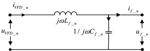
Figure 2. Filter u-phase model.

Figure 3

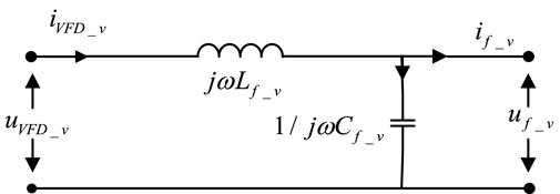
Figure 3. Filter v-phase model.

Figure 4

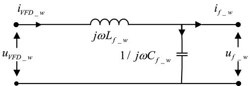
Figure 4. w-Phase model of filter.

For the long cable and the sinusoidal wave filter π-network model shown in Figure 1, since the power supply system is a balanced three-phase network system, it can be represented by a two-port π-network model. As shown in Figures 2–4 and Figures 5–7, they respectively represent the two-port impedance π-network model of the sinusoidal wave filter in the power supply system and the two-port impedance π-network model of the long cable. The sinusoidal wave filter model and the long cable model shown in Figures 2–4 and Figures 5–7 are balanced three-phase network systems, so the parameters of each phase are equal, and we have:

$L_{f\_u}=L_{f\_v}=L_{f\_w}=L_f(1)$

$C_{f\_u}=C_{f\_v}=C_{f\_w}=C_f(2)$

$R_{c\_u}=R_{c\_v}=R_{c\_w}=R_c(3)$

$L_{c\_u}=L_{c\_v}=L_{c\_w}=L_c(4)$

$C_{c\_u}=C_{c\_v}=C_{c\_w}=C_c(5)$

Figure 5

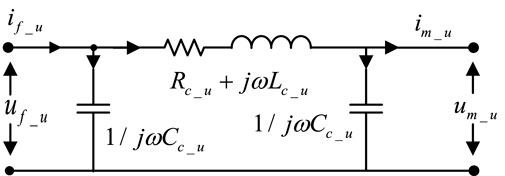
Figure 5. Long cable u-phase two-port network.

Figure 6

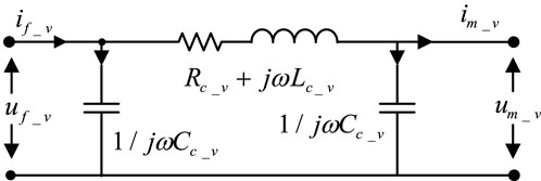
Figure 6. Long cable v-phase two-port network.

Figure 7

Figure 7. Long cable w-phase two-port network.

2.1 Model of filters

The circuit diagram of the filter is shown in Figures 2–4. Figure 2 shows the structural diagram of the filter’s u-port, which can be derived based on Kirchhoff’s voltage and current laws.

$\left\{\begin{array}{l}{u}_{VF{D}_u}=u_{f_u}+j\omega L_{f_u}·i_{VF{D}_u}\\ i_{VF{D}_u}=i_{f_u}+\frac{u_{f_u}}{\frac{1}{j\omega C_{f_u}}}\end{array}\right.(6)$

The inductive reactance and capacitive reactance in Figure 1 are:

$Z_{F_u}=j\omega L_{f_u}(7)$

$Z_{R_u}=\frac{1}{j\omega C_{f_u}}(8)$

Substituting Equation 7 and Equation 8 into Equation 6 yields:

$\left\{\begin{array}{l}{u}_{f_u}=u_{VF{D}_u}-Z_{F_u}·i_{VF{D}_u}\\ i_{f_u}=i_{VF{D}_u}-\frac{u_{f_u}}{Z_{R_u}}\end{array}\right.(9)$

Calculation shows:

$\left\{\begin{array}{l}{u}_{f_u}=u_{VF{D}_u}-Z_{F_u}·i_{VF{D}_u}\\ i_{f_u}=-\frac{u_{VF{D}_u}}{Z_{R_u}}+\left(1+\frac{Z_{F_u}}{Z_{R_u}}\right)i_{VF{D}_u}\end{array}\right.(10)$

From Equation 10, the function of the filter can be calculated as follows:

$\left[\begin{array}{c}{u}_{f_u}\\ i_{f_u}\end{array}\right]=\left[\begin{array}{cc}1& -Z_{F_u}\\ -\frac{1}{Z_{R_u}}& 1+\frac{Z_{F_u}}{Z_{R_u}}\end{array}\right]\left[\begin{array}{c}{u}_{VF{D}_u}\\ i_{VF{D}_u}\end{array}\right](11)$

Similarly, the functional relationships of the other two phases can be obtained:

$\left[\begin{array}{c}{u}_{f_v}\\ i_{f_v}\end{array}\right]=\left[\begin{array}{cc}1& -Z_{F_v}\\ -\frac{1}{Z_{R_v}}& 1+\frac{Z_{F_v}}{Z_{R_v}}\end{array}\right]\left[\begin{array}{c}{u}_{VF{D}_v}\\ i_{VF{D}_v}\end{array}\right](12)$

$\left[\begin{array}{c}{u}_{f_w}\\ i_{f_w}\end{array}\right]=\left[\begin{array}{cc}1& -Z_{F_w}\\ -\frac{1}{Z_{R_w}}& 1+\frac{Z_F}{Z_{R_w}}\end{array}\right]\left[\begin{array}{c}{u}_{VF{D}_w}\\ i_{VF{D}_w}\end{array}\right](13)$

Equation 11, Equation 12, and Equation 13 represent the transfer function of the filter. Calculate the output voltage and current through the input voltage and current of the filter.

2.2 Model of long cables

The network model of each phase at the two ports of the long cable shown in Figure 1 can also be converted into a circuit schematic diagram in the time domain, as shown in Figures 5–7. Figure 5 shows the circuit structure diagram of the two ports of the u-phase of the long cable. According to Kirchhoff’s voltage and current laws, we can obtain

$\left\{\begin{array}{l}{u}_{f\_u}=\left(i_{f\_u}-\frac{u_{f\_u}}{\frac{1}{j\omega C_{c\_u}}}\right)·\left(R_{c-u}+j\omega L_{c\_u}\right)+u_{m\_u}\\ i_{f\_u}=\frac{u_{f\_u}}{\frac{1}{j\omega C_{c\_u}}}+\frac{u_{m\_u}}{\frac{1}{j\omega C_{c\_u}}}+i_{m\_u}\end{array}\right.(14)$

Let the inductive reactance and capacitive reactance in the circuit structure diagram of the two ports of the u-phase of the long cable be:

$Z_{L\_u}=R_{c\_u}+j\omega L_{c\_u}(15)$

$Z_{C\_u}=\frac{1}{j\omega C_{c\_u}}(16)$

Substitute Equations 15, 16 into Equation 14 to obtain

$\left\{\begin{array}{l}{u}_{f\_u}=\left(i_{f\_u}-\frac{u_{f\_u}}{Z_{C\_u}}\right)·Z_{L\_u}+u_{m\_u}\\ i_{f\_u}=\frac{u_{f\_u}}{Z_{C\_u}}+\frac{u_{m\_u}}{Z_{C\_u}}+i_{m\_u}\end{array}\right.(17)$

After arrangement,

$\left\{\begin{array}{l}{u}_{m\_u}=\left(1+\frac{Z_{L\_u}}{Z_{C\_u}}\right)·u_{f\_u}-Z_{L\_u}·i_{f\_u}\\ i_{m\_u}=\left(\frac{-Z_{L\_u}-2Z_{C\_u}}{Z_{C\_u}^2}\right)·u_{f\_u}+\left(1+\frac{Z_{L\_u}}{Z_{C\_u}}\right)·i_{f\_u}\end{array}\right.(18)$

From Equation 18, the functional relationship between the two-port parameters of the u-phase of the long cable can be deduced.

$\left[\begin{array}{c}{u}_{m\_u}\\ i_{m\_u}\end{array}\right]=\left[\begin{array}{cc}1+\frac{Z_{L\_u}}{Z_{C\_u}}& -Z_{L\_u}\\ \frac{-Z_{L\_u}-2Z_{C\_u}}{Z_{C\_u}^2}& 1+\frac{Z_{L\_u}}{Z_{C\_u}}\end{array}\right]\left[\begin{array}{c}{u}_{f\_u}\\ i_{f\_u}\end{array}\right](19)$

Similarly, the functional relationships of the two-port parameters of the v-phase and w-phase of the long cable can be obtained.

$\left[\begin{array}{c}{u}_{m\_v}\\ i_{m\_v}\end{array}\right]=\left[\begin{array}{cc}1+\frac{Z_{L\_v}}{Z_{C\_v}}& -Z_{L\_v}\\ \frac{-Z_{L\_u}-2Z_{C\_v}}{Z_{C\_v}^2}& 1+\frac{Z_{L\_v}}{Z_{C\_v}}\end{array}\right]\left[\begin{array}{c}{u}_{f\_v}\\ i_{f\_v}\end{array}\right](20)$

$\left[\begin{array}{c}{u}_{m\_w}\\ i_{m\_w}\end{array}\right]=\left[\begin{array}{cc}1+\frac{Z_{L\_w}}{Z_{C\_w}}& -Z_{L\_w}\\ \frac{-Z_{L\_u}-2Z_{C\_w}}{Z_{C\_w}^2}& 1+\frac{Z_{L\_w}}{Z_{C\_w}}\end{array}\right]\left[\begin{array}{c}{u}_{f\_w}\\ i_{f\_w}\end{array}\right](21)$

Since the long cable in the power supply system is a three-phase balanced system, substituting Equation 3, Equation 4 and Equation 5 into Equation 7 and Equation 8, the inductive reactance and capacitive reactance in the three-phase two-port network model of the long cable shown in Figures 5–7 are obtained as follows:

$Z_L=R_c+j\omega L_c(22)$

$Z_C=\frac{1}{j\omega C_c}(23)$

Substituting Equations 22, 23 into Equations 19–21, we can obtain the functional relationship between the input and output parameters of the two ports of the long cable:

$\left[\begin{array}{c}{u}_{m\_u}\\ i_{m\_u}\end{array}\right]=\left[\begin{array}{cc}1+\frac{Z_L}{Z_C}& -Z_L\\ \frac{-Z_L-2Z_C}{Z_C^2}& 1+\frac{Z_L}{Z_C}\end{array}\right]\left[\begin{array}{c}{u}_{f\_u}\\ i_{f\_u}\end{array}\right](24)$

$\left[\begin{array}{c}{u}_{m\_v}\\ i_{m\_v}\end{array}\right]=\left[\begin{array}{cc}1+\frac{Z_L}{Z_C}& -Z_L\\ \frac{-Z_L-2Z_C}{Z_C^2}& 1+\frac{Z_L}{Z_C}\end{array}\right]\left[\begin{array}{c}{u}_{f\_v}\\ i_{f\_v}\end{array}\right](25)$

$\left[\begin{array}{c}{u}_{m\_w}\\ i_{m\_w}\end{array}\right]=\left[\begin{array}{cc}1+\frac{Z_L}{Z_C}& -Z_L\\ \frac{-Z_L-2Z_C}{Z_C^2}& 1+\frac{Z_L}{Z_C}\end{array}\right]\left[\begin{array}{c}{u}_{f\_w}\\ i_{f\_w}\end{array}\right](26)$

If the length of the cable in the power supply system is l_c (km), then the functional relationship between the input and output parameters of the two ports of a long cable of any length can be obtained as follows:

$\left[\begin{array}{c}{u}_{m\_u}\\ i_{m\_u}\end{array}\right]={\left[\begin{array}{cc}1+\frac{Z_L}{Z_C}& -Z_L\\ \frac{-Z_L-2Z_C}{Z_C^2}& 1+\frac{Z_L}{Z_C}\end{array}\right]}^{l_c}\left[\begin{array}{c}{u}_{f\_u}\\ i_{f\_u}\end{array}\right](27)$

$\left[\begin{array}{c}{u}_{m\_v}\\ i_{m\_v}\end{array}\right]={\left[\begin{array}{cc}1+\frac{Z_L}{Z_C}& -Z_L\\ \frac{-Z_L-2Z_C}{Z_C^2}& 1+\frac{Z_L}{Z_C}\end{array}\right]}^{l_c}\left[\begin{array}{c}{u}_{f\_v}\\ i_{f\_v}\end{array}\right](28)$

$\left[\begin{array}{c}{u}_{m\_w}\\ i_{m\_w}\end{array}\right]={\left[\begin{array}{cc}1+\frac{Z_L}{Z_C}& -Z_L\\ \frac{-Z_L-2Z_C}{Z_C^2}& 1+\frac{Z_L}{Z_C}\end{array}\right]}^{l_c}\left[\begin{array}{c}{u}_{f\_w}\\ i_{f\_w}\end{array}\right](29)$

Equations 27–29 are the functional relationships between the input and output voltage and current signals at the two ports of the long cable in the power supply system shown in Figure 1 and the distributed parameters of the long cable. The three-phase voltage and three-phase current signals input to the submersible electric pump can be calculated from the voltage and current signals output from the sinusoidal wave filter side.

2.3 Comprehensive mathematical model of sinusoidal wave filter and long cable

Due to the existence of the long cable, various control strategies in the power supply system often cannot achieve satisfactory control effects. Especially for the vector control algorithm, accurate three-phase current signals and three-phase voltage signals of the stator of the induction motor are required. Therefore, it is necessary to calculate the three-phase voltage and current signals at the submersible electric pump end from the three-phase voltage and three-phase current signals output measured at the VFD’s side.

Therefore, substituting Equations 11–13 into Equations 27–29 respectively, we get

$\left[\begin{array}{c}{u}_{m\_u}\\ i_{m\_u}\end{array}\right]={\left[\begin{array}{cc}1+\frac{Z_L}{Z_C}& -Z_L\\ \frac{-Z_L-2Z_C}{Z_C^2}& 1+\frac{Z_L}{Z_C}\end{array}\right]}^{l_c}\left[\begin{array}{cc}1& -Z_F\\ -\frac{1}{Z_R}& 1+\frac{Z_F}{Z_R}\end{array}\right]\left[\begin{array}{c}{u}_{VFD\_u}\\ i_{VFD\_u}\end{array}\right](30)$

$\left[\begin{array}{c}{u}_{m\_v}\\ i_{m\_v}\end{array}\right]={\left[\begin{array}{cc}1+\frac{Z_L}{Z_C}& -Z_L\\ \frac{-Z_L-2Z_C}{Z_C^2}& 1+\frac{Z_L}{Z_C}\end{array}\right]}^{l_c}\left[\begin{array}{cc}1& -Z_F\\ -\frac{1}{Z_R}& 1+\frac{Z_F}{Z_R}\end{array}\right]\left[\begin{array}{c}{u}_{VFD\_v}\\ i_{VFD\_v}\end{array}\right](31)$

$\left[\begin{array}{c}{u}_{m\_w}\\ i_{m\_w}\end{array}\right]={\left[\begin{array}{cc}1+\frac{Z_L}{Z_C}& -Z_L\\ \frac{-Z_L-2Z_C}{Z_C^2}& 1+\frac{Z_L}{Z_C}\end{array}\right]}^{l_c}\left[\begin{array}{cc}1& -Z_F\\ -\frac{1}{Z_R}& 1+\frac{Z_F}{Z_R}\end{array}\right]\left[\begin{array}{c}{u}_{VFD\_w}\\ i_{VFD\_w}\end{array}\right](32)$

Through Equations 30–32, the actual input three-phase voltage and three-phase current signal values at the electric submersible pump end can be calculated from the three-phase voltage and three-phase current signals measured on the VFD’s side.

3 Improved vector control algorithm

3.1 Mathematical model of induction motor

3.1.1 Induction motor model based on rotor flux orientation

The basic idea of the vector control algorithm oriented by the rotor flux is to obtain an equivalent DC motor model in the synchronous rotating orthogonal reference coordinate system through an appropriate coordinate transformation. By analogy with DC motor control methods, the electromagnetic torque T_e and the magnitude of the rotor flux ψ_r are controlled independently. Then, the control quantities in the rotating orthogonal coordinate system are inverse-transformed to obtain the corresponding control quantities in the three-phase coordinate system for implementation of control. The motor model after rotor flux orientation is as follows:

3.1.1.1 Stator Voltage Equation

$\left\{\begin{array}{l}{u}_{sd}=R_s{i}_{sd}+p\sigma L_s{i}_{sd}-\sigma L_s{\omega }_1{i}_{sq}+p\frac{L_m}{L_r}{\psi }_r\\ u_{sq}=R_s{i}_{sq}+p\sigma L_s{i}_{sq}+\sigma L_s{\omega }_1{i}_{sd}+\frac{L_m}{L_r}{\omega }_1{\psi }_r\end{array}\right.(33)$

In the equation, u_sd and u_sq are the stator voltage components of the motor in the d-q rotating reference frame (V); i_sd and i_sq are the stator current components of the motor in the d-q rotating reference frame (A); ω₁ is the synchronous rotation angular velocity (r/min); p is the differential operator; L_m, L_s, L_r are the equivalent mutual inductance between the stator and the rotor (H), the equivalent self-inductance of the stator (H) and the equivalent self-inductance of the rotor (H) respectively; σ is the leakage coefficient; R_S is the stator resistance of the motor (Ω); ψ_r is the magnitude of the rotor flux linkage.

3.1.1.2 Torque Equation

$T_e=\frac{3n_p{L}_m}{2L_r}{\psi }_r{i}_{sq}(34)$

Where: Te is the electromagnetic torque of the motor (N·m); n_p is the number of pole pairs of the motor.

3.1.1.3 Feedforward Decoupling Voltage Equation

$\left\{\begin{array}{l}{u}_{sd}^{*}=-{\omega }_1\sigma L_s{i}_{sq}^{*}\\ u_{sq}^{*}={\omega }_1\sigma L_s{i}_{sd}^{*}+{\omega }_1\frac{L_m}{L_r}{\psi }_r^{*}\end{array}\right.(35)$

${\omega }_1=p\theta (36)$

In the equation: ${\psi }_r*$ is the reference magnetic flux amplitude of the motor rotor; $i_{sd}*$ and $i_{sq}*$ are the reference stator current components (A) in the d-q rotating reference coordinate system, respectively; $u_{sd}*$ and $u_{sq}*$ are the coupling term voltages, respectively; θ is the rotor flux phase angle.

3.1.2 Model Reference Adaptive System

The speed sensorless control technology adopted in this paper is based on the Model Reference Adaptive System (MRAS) of rotor flux linkage. This method uses the current model as the adjustable model and the voltage model as the reference model. The deviation between the outputs of the two models forms an adaptive system to correct the speed in the adjustable model, where the output value of the adaptive regulator becomes the observed speed value. The system equations are as follows:

3.1.2.1 Voltage model (reference model)

$\left\{\begin{array}{l}{\psi }_{r\alpha }=\frac{L_r}{L_m}\left[\int \left(u_{s\alpha }-R_s{i}_{s\alpha }\right)dt-\sigma L_s{i}_{s\alpha }\right]\\ {\psi }_{r\beta }=\frac{L_r}{L_m}\left[\int \left(u_{s\beta }-R_s{i}_{s\beta }\right)dt-\sigma L_s{i}_{s\beta }\right]\end{array}\right.(37)$

In the equation: ψ_rα and ψ_rβ represent the motor rotor flux linkage components (voltage model) (Wb) in the α-β stationary reference coordinate system; u_sα and u_sβ represent the motor stator voltage components (V) in the α-β stationary reference coordinate system; i_sα and i_sβ represent the motor stator current components (A) in the α-β stationary coordinate system.

3.1.2.2 Current model (adjustment model)

$\left\{\begin{array}{c}{\psi }_{r\alpha }^r=\int \left(-\frac{R_r}{L_r}{\psi }_{r\alpha }^r-\omega {\psi }_{r\beta }^r+L_m\frac{R_r}{L_r}{i}_{s\alpha }\right)dt\\ {\psi }_{r\beta }^r=\int \left(-\frac{R_r}{L_r}{\psi }_{r\beta }^r+\omega {\psi }_{r\alpha }^r+L_m\frac{R_r}{L_r}{i}_{s\beta }\right)dt\end{array}\right.(38)$

In the equation: ${\psi }_{r\alpha }^r$ and ${\psi }_{r\beta }^r$ represent the motor rotor flux components (current model) (Wb) in the α-β coordinate system; R_r denotes the motor rotor resistance (Ω); ω indicates the estimated motor angular velocity (r/min).

3.1.2.3 Error equation

$e_{speed}={\psi }_{r\beta }{\psi }_{r\alpha }^r-{\psi }_{r\alpha }{\psi }_{r\beta }^r(39)$

3.1.2.4 Estimated speed calculation

$\omega =\left(K_{p\_est}+\frac{K_{i\_est}}{s}\right)e_{speed}(40)$

In the equation: k_{p_est} and k_{i_est} are the motor speed PI controller constants respectively.

3.1.2.5 Rotor flux linkage amplitude and rotor flux phase angle

${\psi }_r=\sqrt{{\psi }_{r\alpha }^2+{\psi }_{r\beta }^2}(41)$

$\theta ={\mathit{sin}}^{-1}\frac{{\psi }_{r\beta }}{{\psi }_{r\alpha }}(42)$

3.1.3 Conventional speed sensorless vector control algorithm for power supply systems

The conventional speed sensorless vector control algorithm for power supply systems is a speed closed-loop control system. Through coordinate transformation, speed and flux observers, it achieves speed estimation, decoupling of electromagnetic torque and rotor flux, as well as closed-loop control of electromagnetic torque, rotor flux, speed, and current.

However, in this control algorithm, the estimation of speed ω, the magnitude of rotor flux ψ_r, rotor phase angle θ, and the calculation of electromagnetic torque T_e are all based on the measured three-phase voltage and current signals output by the inverter. The measured three-phase voltage and current signals from the inverter side are directly treated as the motor’s input three-phase voltage and current signals and applied to the feedforward decoupling and motor stator voltage generation unit shown in Section 3.1.1, as well as the MRAS-based speed estimation and flux calculation unit shown in Section 3.1.2. The influence of long cable distributed parameters on the motor-side three-phase voltage and current signals is completely disregarded.

3.2 Design of speed sensorless vector control algorithm for power supply system based on lyapunov stability theory

3.2.1 Improved speed sensorless vector control algorithm

To address the influence of sinusoidal wave filters and distributed parameters of long cables, this paper proposes a speed sensorless vector control algorithm for the power supply system based on Lyapunov stability theory, utilizing a comprehensive mathematical model of sinusoidal wave filters and the two-port characteristics of long cables. This algorithm is primarily designed for motor loads connected via long cables, and its control system block diagram is shown in Figure 8. The proposed control algorithm employs the three-phase voltage and current signals output by the inverter to calculate the precise motor terminal voltage and current signals using the comprehensive mathematical model of sinusoidal wave filters and long cables in the α-β stationary reference frame. These calculated motor terminal signals are then used to estimate the speed, rotor flux amplitude, and rotor flux phase angle of the induction motor, rather than directly using the measured inverter output signals. This approach enables the accurate construction of a rotor flux linkage model, achieving precise observation of rotor flux linkage and speed identification, as well as closed-loop control of torque, flux, and current.

Figure 8

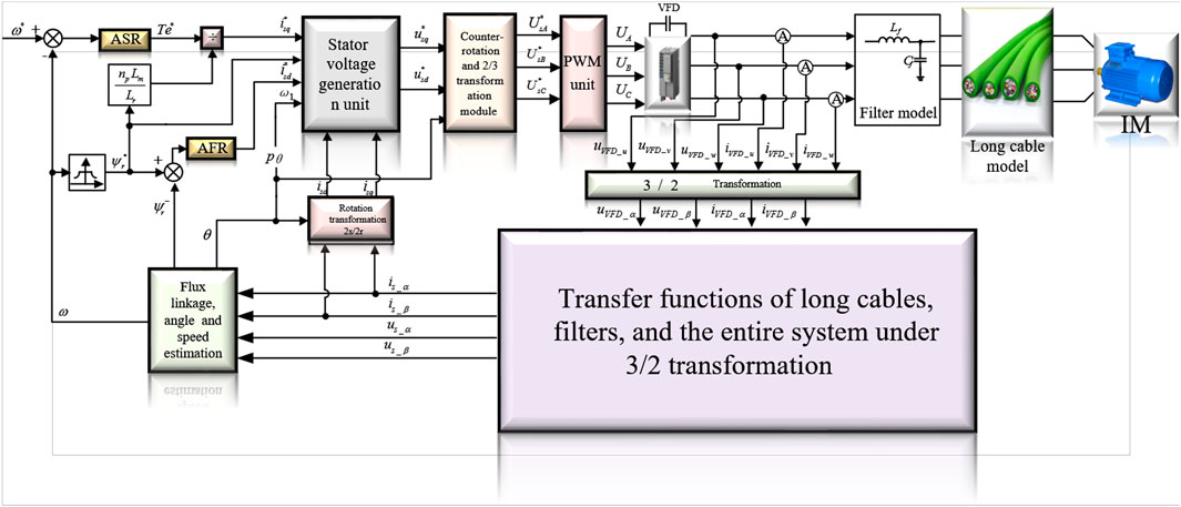
Figure 8. Vector control algorithm for long cables.

3.2.2 Stability analysis of the speed sensorless vector control algorithm

As shown in Figure 8, the improved speed sensorless vector control algorithm independently controls the electromagnetic torque Te and the rotor flux amplitude ψ_r. To obtain an accurate mathematical model for the improved algorithm, the motor terminal stator voltage components u_{s_d} and u_{s_q}, the motor terminal stator current components i_{s_d} and i_{s_q}, and the rotor flux amplitude ψ_{r_r}, calculated in the d-q rotating reference frame based on the comprehensive mathematical model of sinusoidal wave filters and long cables, must be substituted into the rotor flux-oriented motor model (Equations 33, 34). This yields an accurate dynamic mathematical model of the rotor flux-oriented induction motor based on the comprehensive mathematical model of sinusoidal wave filters and long cables.

$\stackrel{·}{i_{s\_d}}=\beta i_{s\_d}+{\omega }_1{i}_{s\_q}+\frac{L_m}{\sigma L_s{L}_r{T}_r}{\psi }_{r\_r}+\frac{1}{\sigma L_s}{u}_{s\_d}(43)$

$\stackrel{·}{i_{s\_q}}=-{\omega }_1{i}_{s\_d}+\beta i_{s\_q}-\frac{L_m}{\sigma L_s{L}_r}\omega {\psi }_{r\_r}+\frac{1}{\sigma L_s}{u}_{s\_q}(44)$

In the equation $\beta =-\frac{R_s{L}_r^2+R_r{L}_m^2}{\sigma L_s{L}_r^2}$,T_r is motor rotor time.

The rotor flux linkage function can be expressed as:

$\stackrel{·}{{\psi }_{r_r}}=-\frac{1}{T_r}{\psi }_{r_r}+\frac{L_m}{T_r}{i}_{s_d}(45)$

The electromagnetic torque equation can be expressed as:

$T_e=\frac{3n_p{L}_m}{2L_r}{\psi }_{r_r}{i}_{s_q}(46)$

The dynamic function of the motor is:

$\stackrel{·}{x}=J\left(x\right)+g·u_{s_{d}q}(47)$

The state variables in the transfer function are:

$x={\left[\begin{array}{ccc}{i}_{s_d}& i_{s_q}& {\psi }_{r_r}\end{array}\right]}^T(48)$

The input transfer function is:

$u_{s_{d}q}={\left[\begin{array}{cc}{u}_{s_d}& u_{s_q}\end{array}\right]}^T(49)$

There is

$g={\left[\begin{array}{c}\begin{array}{ccc}\frac{1}{\sigma L_s}& 0& 0\end{array}\\ \begin{array}{ccc}0& \frac{1}{\sigma L_s}& 0\end{array}\end{array}\right]}^T(50)$

$J\left(x\right)=\left[\begin{array}{ccc}\beta & {\omega }_1& \frac{L_m}{\sigma L_s{L}_r{T}_r}\\ -{\omega }_1& \beta & \frac{L_m\omega }{\sigma L_s{T}_r}\\ \frac{L_m}{T_r}& 0& -\frac{1}{T_r}\end{array}\right]\left[\begin{array}{c}{i}_{s_d}\\ i_{s_q}\\ {\psi }_{r_r}\end{array}\right](51)$

By analyzing the stability of this transfer function, an improved equation for long cable conditions can be derived. Substituting the voltages u_{s_α} and u_{s_β} and the currents i_{s_α} and i_{s_β} into Equation 37 yields:

$\left\{\begin{array}{l}{\psi }_{r\alpha }=\frac{L_r}{L_m}\left[\int \left(u_{s\alpha }-R_s{i}_{s\alpha }\right)dt-\sigma L_s{i}_{s\alpha }\right]\\ {\psi }_{r\beta }=\frac{L_r}{L_m}\left[\int \left(u_{s\beta }-R_s{i}_{s\beta }\right)dt-\sigma L_s{i}_{s\beta }\right]\end{array}\right.(52)$

In the equation, ψ_{r_α} and ψ_{r_β} are the two-phase magnetic fluxes calculated from the output voltage and current of the VFD.

${\psi }_{r_r}=\sqrt{{\psi }_{r_{\alpha }}^2+{\psi }_{r_{\beta }}^2}(53)$

In the equation, ψ_{r_r} is the calculated amplitude of the magnetic flux linkage. From this, the transfer function after the Park transformation can be derived.

$\begin{array}{c}\left[\begin{array}{c}{u}_{s_d}\\ i_{s_d}\end{array}\right]=\left[\begin{array}{cc}\mathit{cos}\theta & \mathit{sin}\theta \\ -\mathit{sin}\theta & \mathit{cos}\theta \end{array}\right]{\left[\begin{array}{cc}1+\frac{Z_L}{Z_C}& -Z_L\\ \frac{-Z_L-2Z_C}{Z_C^2}& 1+\frac{Z_L}{Z_C}\end{array}\right]}^{l_c}\\ \left[\begin{array}{cc}1& -Z_F\\ -\frac{1}{Z_R}& 1+\frac{Z_F}{Z_R}\end{array}\right]\left[\begin{array}{c}{u}_{VF{D}_{\alpha }}\\ i_{VF{D}_{\alpha }}\end{array}\right]\end{array}(54)$

$\begin{array}{c}\left[\begin{array}{c}{u}_{s_q}\\ i_{s_q}\end{array}\right]=\left[\begin{array}{cc}\mathit{cos}\theta & \mathit{sin}\theta \\ -\mathit{sin}\theta & \mathit{cos}\theta \end{array}\right]{\left[\begin{array}{cc}1+\frac{Z_L}{Z_C}& -Z_L\\ \frac{-Z_L-2Z_C}{Z_C^2}& 1+\frac{Z_L}{Z_C}\end{array}\right]}^{l_c}\\ \left[\begin{array}{cc}1& -Z_F\\ -\frac{1}{Z_R}& 1+\frac{Z_F}{Z_R}\end{array}\right]\left[\begin{array}{c}{u}_{VF{D}_{\beta }}\\ i_{VF{D}_{\beta }}\end{array}\right]\end{array}(55)$

Equations 54, 55 are the output voltage and current of the filter model and the long cable model in the d-q coordinate system. By incorporating them into the vector control algorithm, the response characteristics of the vector control algorithm under long cable conditions can be improved. From this, the motor stator voltages u_{s_d} and u_{s_q}, the motor stator currents i_{s_d} and i_{s_q}, and the motor rotor flux linkage ψ_{r_r} can be obtained. Thus, the parameter model is given as:

$\begin{array}{c}\left[\begin{array}{cc}{K}_1& K_2\\ K_3& K_4\end{array}\right]=\left[\begin{array}{cc}\mathit{cos}\theta & \mathit{sin}\theta \\ -\mathit{sin}\theta & \mathit{cos}\theta \end{array}\right]{\left[\begin{array}{cc}1+\frac{Z_L}{Z_C}& -Z_L\\ \frac{-Z_L-2Z_C}{Z_C^2}& 1+\frac{Z_L}{Z_C}\end{array}\right]}^{l_c}\\ \left[\begin{array}{cc}1& -Z_F\\ -\frac{1}{Z_R}& 1+\frac{Z_F}{Z_R}\end{array}\right]\end{array}(56)$

Then Equations 54, 55 are transformed into:

$\left[\begin{array}{c}{u}_{s_d}\\ i_{s_d}\end{array}\right]=\left[\begin{array}{cc}{K}_1& K_2\\ K_3& K_4\end{array}\right]\left[\begin{array}{c}{u}_{VF{D}_{\alpha }}\\ i_{VF{D}_{\alpha }}\end{array}\right](57)$

$\left[\begin{array}{c}{u}_{s_q}\\ i_{s_q}\end{array}\right]=\left[\begin{array}{cc}{K}_1& K_2\\ K_3& K_4\end{array}\right]\left[\begin{array}{c}{u}_{VF{D}_{\beta }}\\ i_{VF{D}_{\beta }}\end{array}\right](58)$

As shown in Figure 8, the output of the control algorithm is torque and rotor flux linkage:

$\left\{\begin{array}{c}{y}_1=T_e\\ y_2={\psi }_{r_r}\end{array}\right.(59)$

Define the deviation between torque and rotor flux linkage as:

$\left\{\begin{array}{l}{e}_1={T*}_e-T_e\\ e_2={\psi }_{r_r}^{*}-{\psi }_{r_r}\end{array}\right.(60)$

In Equation 60, e₁ and e₂ represent the errors of torque and rotor flux linkage, respectively, where $T_e^{*}$, ${\psi }_{r_r}^{*}$ denote the desired torque and desired rotor flux linkage. Thus, we have:

$\stackrel{·}{T_e^{*}}=0(61)$

$\stackrel{·}{{\psi }_{r_r}^{*}}=0(62)$

The input-output relationship of the control system shown in Figure 8 is:

$\stackrel{·}{e}=\left[\begin{array}{c}{\stackrel{·}{e}}_1\\ {\stackrel{·}{e}}_2\end{array}\right]=\left[\begin{array}{c}{J}_1\left(x\right)\\ J_2\left(x\right)\end{array}\right]+\left[\begin{array}{c}{g}_1\\ g_2\end{array}\right]\left[\begin{array}{c}{u}_{s_d}\\ u_{s_q}\end{array}\right](63)$

Differentiating the torque and rotor flux deviation shown in Equation 60 yields:

${\stackrel{·}{e}}_1=\stackrel{·}{T_e^{*}}-\stackrel{·}{T_e}(64)$

${\stackrel{·}{e}}_2=\stackrel{·}{{\psi }_{r_r}^{*}}-\stackrel{·}{{\psi }_{r_r}}(65)$

Substituting Equations 46 and 61 and Equations 45 and 62 into Equations 64, 65 respectively, we can calculate:

${\stackrel{·}{e}}_1=-\frac{3n_p{L}_m}{2L_r}{\psi }_{r_r}\stackrel{·}{i_{s_q}}(66)$

${\stackrel{·}{e}}_2=\frac{1}{T_r}{\psi }_{r_r}-\frac{L_m}{T_r}{i}_{s_d}(67)$

Substituting Equation 44 into Equation 66, the torque deviation differential is calculated as:

${\stackrel{·}{e}}_1=\frac{3n_p{L}_m}{2L_r}{\psi }_{r_r}\left({\omega }_1{i}_{s_d}-\beta i_{s_q}+\frac{L_m}{\sigma L_s{L}_r}\omega {\psi }_{r_r}-\frac{1}{\sigma L_s}{u}_{s_q}\right)(68)$

Substituting the torque and rotor flux deviation differentials from Equations 67, 68 into Equation 69 yields the input-output relationship as:

$\begin{array}{c}\stackrel{·}{e}=\left[\begin{array}{c}{\stackrel{·}{e}}_1\\ {\stackrel{·}{e}}_2\end{array}\right]=\left[\begin{array}{c}\frac{3n_p{L}_m{\psi }_{r_r}}{2L_r}\left({\omega }_1{i}_{s_d}-\beta i_{s_q}+\frac{\omega L_m{\psi }_{r_r}}{\sigma L_s{L}_r}\right)\\ \frac{1}{T_r}{\psi }_{r_r}-\frac{L_m}{T_r}{i}_{s_d}\end{array}\right]\\ +\left[\begin{array}{cc}0& -\frac{3n_p{L}_m{\psi }_{r_r}}{2\sigma L_s{L}_r}\\ 0& 0\end{array}\right]\left[\begin{array}{c}{u}_{s_d}\\ u_{s_q}\end{array}\right]\end{array}(69)$

In Equation 69, the voltages in the d-q coordinate system are u_{s_d}, u_{s_q,} and the motor stator currents are i_{s_d}, i_{s_q}. The model calculated through Equations 57, 58 is the final model, while the motor rotor flux linkage ψ_{r_r} is calculated by Equation 53. By substituting the motor voltages, currents, and rotor flux linkage into Equations 67, 68, we obtain:

$\begin{array}{c}{\stackrel{·}{e}}_1=\frac{3n_p{L}_m{\psi }_{r_r}}{2L_r}\left(K_4{\omega }_1{i}_{VF{D}_{\alpha }}-\beta K_4{i}_{VF{D}_{\beta }}-\frac{K_2}{\sigma L_s}{i}_{VF{D}_{\beta }}+\frac{\omega L_m{\psi }_{r_r}}{\sigma L_s{L}_r}\right)\\ +\left[\begin{array}{cc}\frac{3n_p{L}_m{\psi }_{r_r}}{2L_r}{K}_3{\omega }_1& -\frac{3n_p{L}_m{\psi }_{r_r}}{2L_r}\left(\beta K_3+\frac{K_1}{\sigma L_s}\right)\end{array}\right]\left[\begin{array}{c}{u}_{VF{D}_{\alpha }}\\ u_{VF{D}_{\beta }}\end{array}\right]\end{array}(70)$

${\stackrel{·}{e}}_2=-\frac{K_4{L}_m}{T_r}{i}_{VF{D}_{\alpha }}+\frac{1}{T_r}{\psi }_{r_r}-\frac{K_3{L}_m}{T_r}{u}_{VF{D}_{\alpha }}(71)$

Substituting Equations 70, 71 into the input-output function mentioned earlier, namely, Equation 69, we obtain

$\begin{array}{l}J\left(x\right)=\left[\begin{array}{c}{J}_1\left(x\right)\\ J_2\left(x\right)\end{array}\right]\\ =\left[\begin{array}{c}\frac{3n_p{L}_m{\psi }_{r_r}}{2L_r}\left(K_4{\omega }_1{i}_{VF{D}_{\alpha }}-\beta K_4{i}_{VF{D}_{\beta }}-\frac{K_2}{\sigma L_s}{i}_{VF{D}_{\beta }}+\frac{\omega L_m{\psi }_{r_r}}{\sigma L_s{L}_r}\right)\\ -\frac{K_4{L}_m}{T_r}{i}_{VF{D}_{\alpha }}+\frac{1}{T_r}{\psi }_{r_r}\end{array}\right]\end{array}(72)$

$g\left(x\right)=\left[\begin{array}{c}{g}_1\\ g_2\end{array}\right]=\left[\begin{array}{cc}\frac{3n_p{L}_m{\psi }_{r_r}}{2L_r}{K}_3{\omega }_1& -\frac{3n_p{L}_m{\psi }_{r_r}}{2L_r}\left(\beta K_3+\frac{K_1}{\sigma L_s}\right)\\ -\frac{K_3{L}_m}{T_r}& 0\end{array}\right](73)$

Then the input-output relationship shown in Figure 8 becomes:

$\stackrel{·}{e}=\left[\begin{array}{c}{\stackrel{·}{e}}_1\\ {\stackrel{·}{e}}_2\end{array}\right]=\left[\begin{array}{c}{J}_1\left(x\right)\\ J_2\left(x\right)\end{array}\right]+g\left(x\right)\left[\begin{array}{c}{u}_{VF{D}_{\alpha }}\\ u_{VF{D}_{\beta }}\end{array}\right](74)$

The motor stator voltages u_{s_d}, u_{s_q} are converted into the motor stator voltages u_{VFD_α,} u_{VFD_β}. From Equation 74, it can be concluded that the effects of long cables and filters can be eliminated.

The matrix g(x) in Equation 75 is derived from the product of the motor flux linkage and the rotor flux linkage. Therefore, g(x) is a non-singular matrix and is not equal to zero, leading to the input as:

$u=\left[\begin{array}{c}{u}_{VF{D}_{\alpha }}\\ u_{VF{D}_{\beta }}\end{array}\right]=g^{-1}\left(x\right)\left(\left[\begin{array}{c}-J_1\left(x\right)\\ -J_2\left(x\right)\end{array}\right]+\left[\begin{array}{c}{u}_1\\ u_2\end{array}\right]\right)(75)$

Where u₁ and u₂ are adjustment input values, and to ensure favorable characteristics, there exists:

$\left[\begin{array}{c}{u}_1\\ u_2\end{array}\right]=\left[\begin{array}{cc}-K_5& 0\\ 0& -K_6\end{array}\right]\left[\begin{array}{c}{\xi }_1\\ {\xi }_2\end{array}\right](76)$

Substituting Equation 75 and Equation 76 into Equation 74 yields

$\stackrel{·}{e}=\left[\begin{array}{c}{\stackrel{·}{e}}_1\\ {\stackrel{·}{e}}_2\end{array}\right]=\left[\begin{array}{cc}-K_5& 0\\ 0& -K_6\end{array}\right]\left[\begin{array}{c}{\xi }_1\\ {\xi }_2\end{array}\right](77)$

K₅ and K₆ both are select appropriate constants, choose the Lyapunov function as:

$V\left(\xi \right)=\frac{1}{2}{\xi }^T\xi >0(78)$

In the equation

${\xi }^T={\left[\begin{array}{cc}{\xi }_1& {\xi }_2\end{array}\right]}^T(79)$

The derivative of the selected Lyapunov function V(ξ) with respect to time is:

$\stackrel{·}{V}\left(\xi \right)=-K_5{\xi }_1^2-K_6{\xi }_2^2(80)$

Since K₅ and K₆ are positive numbers, $\stackrel{·}{V}\left(\xi \right)$ <0, which proves that the improved vector control algorithm proposed in this paper is asymptotically stable.

3.3 Analysis of the changes in long cable parameters over time and the influence of the deep-sea environment on the comprehensive indicators of long cables

The long cable is below 2 km in the deep sea, and the temperature is constant at 2 °C–4 °C. In the 1 km deep-sea area, the hydrostatic pressure of the long cable reaches 10 MPa. Below 2 km depth, the pressure increases by about 1 atm for every 10 m of water depth. The humidity of long cables is close to 100% in the deep sea, the salt content in seawater is about 3.5%, and the pH value is between 7.5 and 8.4. It is necessary to calculate the coefficient of influence on resistance, capacitance, and inductance to quantify the influence on long cable parameters.

3.3.1 Quantitative analysis of the sensitivity of long cable parameters to time

Suppose P(t) describes the change of R, L, C, over time t. This model is affected by multiple deep-sea environmental factors $x_1\left(t\right),x_2\left(t\right),\cdots ,x_n\left(t\right)$, can be expressed as:

$P\left(t\right)=f\left(x_1\left(t\right),x_2\left(t\right),\cdots ,x_n\left(t\right),t\right)(81)$

To analyze the sensitivity of the proposed method to the time-varying cable parameters, we introduce the sensitivity coefficient $S_{P,x_i}$, which represents the sensitivity of parameter P to the environmental factor $x_i$. The sensitivity coefficient can be defined by partial derivatives:

$S_{P,x_i}=\frac{\partial P}{\partial x_i}·\frac{x_i}{P}(82)$

By calculating the sensitivity coefficients, we can determine which environmental factors have the most significant impact on cable parameters.

To consider the influence of time factors, we can further calculate the rate of change of the sensitivity coefficient concerning time $d{S}_{P,x_i}$:

$\frac{d{S}_{P,x_i}}{dt}=\frac{d}{dt}\left(\frac{\partial P}{\partial x_i}·\frac{x_i}{P}\right)(83)$

Specifically, let the time-varying parameters R, C, and L of the long cable in the deep-sea environment be R(t), C(t), and L(t), respectively. In the deep-sea environment, factors such as temperature, pressure, and humidity can affect the resistivity of the long cable conductor, thereby influencing the resistance. Assuming that the change in resistance over time is related to the temperature T(t), pressure P(t), and humidity H(t), Equations 84–92 can be derived.

$R\left(t\right)=R_0+S_{R,T}T\left(t\right)+S_{R,P}P\left(t\right)+S_{R,H}H\left(t\right)(84)$

Where $R_0$ is the initial resistance, $S_{R,T}$, $S_{R,P}$, $S_{R,H}$ are the coefficients of the influence of temperature, pressure, and humidity on time, respectively.

The capacitance of a long cable is related to the dielectric constant of the insulating material, and the dielectric constant is affected by temperature and humidity. Equation 85 can be derived.

$C\left(t\right)=C_0+S_{C,T}T\left(t\right)+S_{C,H}H\left(t\right)(85)$

Where $C_0$ is the initial capacitance, $S_{C,T}$, $S_{C,H}$ are the coefficients of the influence of temperature and humidity on capacitance respectively.

Inductance is related to the geometric structure and magnetic permeability of the cable. In the deep-sea environment, pressure may cause slight changes in the cable’s geometric structure, thus affecting the inductance.

$L\left(t\right)=L_0+S_{L,P}P\left(t\right)(86)$

Where $L_0$ is the initial inductance, $S_{L,P}$ is the coefficient of the influence of pressure on inductance.

Sensitivity refers to the ratio of the rate of change of a parameter to the rate of change of an influencing factor. The sensitivity of resistance coefficient $S_{R,T}$ of resistance to temperature is defined as:

$S_{R,T}=\frac{\frac{dR\left(t\right)}{R\left(t\right)}}{\frac{dT\left(t\right)}{T\left(t\right)}}=\frac{T\left(t\right)}{R\left(t\right)}\frac{dR\left(t\right)}{dT\left(t\right)}(87)$

The sensitivity coefficient of resistance to pressure $S_{R,P}$ is defined as:

$S_{R,P}=\frac{P\left(t\right)}{R\left(t\right)}\frac{dR\left(t\right)}{dP\left(t\right)}(88)$

The sensitivity coefficient of resistance to humidity $S_{R,H}$ is defined as:

$S_{R,H}=\frac{H\left(t\right)}{R\left(t\right)}\frac{dR\left(t\right)}{dH\left(t\right)}(89)$

Similarly, the sensitivity coefficient of capacitance to temperature $S_{C,T}$ is defined as:

$S_{C,T}=\frac{T\left(t\right)}{C\left(t\right)}\frac{dC\left(t\right)}{dT\left(t\right)}(90)$

The sensitivity coefficient of capacitance to humidity $S_{C,H}$ is defined as:

$S_{C,H}=\frac{H\left(t\right)}{C\left(t\right)}\frac{dC\left(t\right)}{dH\left(t\right)}(91)$

The sensitivity coefficient of inductance to pressure $S_{L,P}$ is defined as:

$S_{L,P}=\frac{P\left(t\right)}{L\left(t\right)}\frac{dL\left(t\right)}{dP\left(t\right)}(92)$

By calculating these parameters, the magnitude and severity of the impacts of various conditions on the R, C, and L of the long cable can be determined.

3.3.2 Lyapunov stability proof of the entire system with the introduction of the time-sensitive long cable model

Substituting the changing parameters R(t), C(t), and L(t) into the long cable Equations 22, 23, we can obtain:

$Z_L\left(t\right)=R\left(t\right)+j\omega L\left(t\right)(93)$

$Z_C\left(t\right)=\frac{1}{j\omega C\left(t\right)}(94)$

Substitute it into Equations 27–29, It can be concluded that the long cable model varying with time is as follows:

$\left[\begin{array}{c}{u}_{m\_u}\\ i_{m\_u}\end{array}\right]={\left[\begin{array}{cc}1+\frac{Z_L\left(t\right)}{Z_C\left(t\right)}& -Z_L\left(t\right)\\ \frac{-Z_L\left(t\right)-2Z_C\left(t\right)}{Z_C^2\left(t\right)}& 1+\frac{Z_L\left(t\right)}{Z_C\left(t\right)}\end{array}\right]}^{l_c}\left[\begin{array}{c}{u}_{f\_u}\\ i_{f\_u}\end{array}\right](95)$

$\left[\begin{array}{c}{u}_{m\_v}\\ i_{m\_v}\end{array}\right]={\left[\begin{array}{cc}1+\frac{Z_L\left(t\right)}{Z_C\left(t\right)}& -Z_L\left(t\right)\\ \frac{-Z_L\left(t\right)-2Z_C\left(t\right)}{Z_C^2\left(t\right)}& 1+\frac{Z_L\left(t\right)}{Z_C\left(t\right)}\end{array}\right]}^{l_c}\left[\begin{array}{c}{u}_{f\_v}\\ i_{f\_v}\end{array}\right](96)$

$\left[\begin{array}{c}{u}_{m\_w}\\ i_{m\_w}\end{array}\right]={\left[\begin{array}{cc}1+\frac{Z_L\left(t\right)}{Z_C\left(t\right)}& -Z_L\left(t\right)\\ \frac{-Z_L\left(t\right)-2Z_C\left(t\right)}{Z_C^2\left(t\right)}& 1+\frac{Z_L\left(t\right)}{Z_C\left(t\right)}\end{array}\right]}^{l_c}\left[\begin{array}{c}{u}_{f\_w}\\ i_{f\_w}\end{array}\right](97)$

Then, Equations 54, 55 become:

$\begin{array}{c}\left[\begin{array}{c}{u}_{s_d}\\ i_{s_d}\end{array}\right]=\left[\begin{array}{cc}\mathit{cos}\theta & \mathit{sin}\theta \\ -\mathit{sin}\theta & \mathit{cos}\theta \end{array}\right]{\left[\begin{array}{cc}1+\frac{Z_L\left(t\right)}{Z_C\left(t\right)}& -Z_L\left(t\right)\\ \frac{-Z_L\left(t\right)-2Z_C\left(t\right)}{Z_C^2\left(t\right)}& 1+\frac{Z_L\left(t\right)}{Z_C\left(t\right)}\end{array}\right]}^{l_c}\\ \left[\begin{array}{cc}1& -Z_F\\ -\frac{1}{Z_R}& 1+\frac{Z_F}{Z_R}\end{array}\right]\left[\begin{array}{c}{u}_{VF{D}_{\alpha }}\\ i_{VF{D}_{\alpha }}\end{array}\right]\end{array}(98)$

$\begin{array}{c}\left[\begin{array}{c}{u}_{s_q}\\ i_{s_q}\end{array}\right]=\left[\begin{array}{cc}\mathit{cos}\theta & \mathit{sin}\theta \\ -\mathit{sin}\theta & \mathit{cos}\theta \end{array}\right]{\left[\begin{array}{cc}1+\frac{Z_L\left(t\right)}{Z_C\left(t\right)}& -Z_L\left(t\right)\\ \frac{-Z_L\left(t\right)-2Z_C\left(t\right)}{Z_C^2\left(t\right)}& 1+\frac{Z_L\left(t\right)}{Z_C\left(t\right)}\end{array}\right]}^{l_c}\\ \left[\begin{array}{cc}1& -Z_F\\ -\frac{1}{Z_R}& 1+\frac{Z_F}{Z_R}\end{array}\right]\left[\begin{array}{c}{u}_{VF{D}_{\beta }}\\ i_{VF{D}_{\beta }}\end{array}\right]\end{array}(99)$

Equation 56 then becomes:

$\begin{array}{l}\left[\begin{array}{cc}{K}_1& K_2\\ K_3& K_4\end{array}\right]=\left[\begin{array}{cc}\mathit{cos}\theta & \mathit{sin}\theta \\ -\mathit{sin}\theta & \mathit{cos}\theta \end{array}\right]{\left[\begin{array}{cc}1+\frac{Z_L\left(t\right)}{Z_C\left(t\right)}& -Z_L\left(t\right)\\ \frac{-Z_L\left(t\right)-2Z_C\left(t\right)}{Z_C^2\left(t\right)}& 1+\frac{Z_L\left(t\right)}{Z_C\left(t\right)}\end{array}\right]}^{l_c}\\ \times \left[\begin{array}{cc}1& -Z_F\\ -\frac{1}{Z_R}& 1+\frac{Z_F}{Z_R}\end{array}\right]\end{array}(100)$

Equation 69 then becomes:

$\begin{array}{c}\stackrel{·}{e}\left(t\right)=\left[\begin{array}{c}{\stackrel{·}{e}}_1\\ {\stackrel{·}{e}}_2\end{array}\right]=\left[\begin{array}{c}\frac{3n_p{L}_m{\psi }_{r_r}\left(t\right)}{2L_r}\left({\omega }_1{i}_{s_d}\left(t\right)-\beta i_{s_q}\left(t\right)+\frac{\omega L_m{\psi }_{r_r\left(t\right)}}{\sigma L_s{L}_r}\right)\\ \frac{1}{T_r}{\psi }_{r_r}\left(t\right)-\frac{L_m}{T_r}{i}_{s_d}\left(t\right)\end{array}\right]\\ +\left[\begin{array}{cc}0& -\frac{3n_p{L}_m{\psi }_{r_r}\left(t\right)}{2\sigma L_s{L}_r}\\ 0& 0\end{array}\right]\left[\begin{array}{c}{u}_{s_d}\\ u_{s_q}\end{array}\right]\end{array}(101)$

Where ${\psi }_{r_r}\left(t\right)$, $i_{s_d}\left(t\right)$, $i_{s_q}\left(t\right)$ are the corresponding flux linkages and d-q axis currents that change with time respectively, $\stackrel{·}{e}\left(t\right)$ is derivative of input-output relationship in chapter 3.2.2 which are under the influence of R(t), C(t), and L(t), Equations 72, 73 become:

$\begin{array}{l}J\left(x\right)=\left[\begin{array}{c}{J}_1\left(x\right)\\ J_2\left(x\right)\end{array}\right]\\ =\left[\begin{array}{c}\frac{3n_p{L}_m{\psi }_{r_r}\left(t\right)}{2L_r}\left(K_4{\omega }_1{i}_{VF{D}_{\alpha }}\left(t\right)-\beta K_4{i}_{VF{D}_{\beta }}\left(t\right)-\frac{K_2}{\sigma L_s}{i}_{VF{D}_{\beta }}\left(t\right)+\frac{\omega L_m{\psi }_{r_r}\left(t\right)}{\sigma L_s{L}_r}\right)\\ -\frac{K_4{L}_m}{T_r}{i}_{VF{D}_{\alpha }\left(t\right)}+\frac{1}{T_r}{\psi }_{r_r}\left(t\right)\end{array}\right]\end{array}(102)$

$g\left(x\right)=\left[\begin{array}{c}{g}_1\\ g_2\end{array}\right]=\left[\begin{array}{cc}\frac{3n_p{L}_m{\psi }_{r_r}\left(t\right)}{2L_r}{K}_3{\omega }_1& -\frac{3n_p{L}_m{\psi }_{r_r}\left(t\right)}{2L_r}\left(\beta K_3+\frac{K_1}{\sigma L_s}\right)\\ -\frac{K_3{L}_m}{T_r}& 0\end{array}\right](103)$

Where $i_{VF{D}_{\alpha }}\left(t\right)$ and $i_{VF{D}_{\beta }}\left(t\right)$ are the inverter current that changes with time under the influence of R(t), C(t), and L(t).

Then, through the derivation in chapter 3.2.2, we can derive the derivative of the input-output relationship $\stackrel{·}{e}\left(t\right)$ with the introduction of time sensitivity.

$\stackrel{·}{e}\left(t\right)=\left[\begin{array}{c}{\stackrel{·}{e}}_1\\ {\stackrel{·}{e}}_2\end{array}\right]=\left[\begin{array}{cc}-K_5& 0\\ 0& -K_6\end{array}\right]\left[\begin{array}{c}{\xi }_1\\ {\xi }_2\end{array}\right](104)$

Finally, through the derivation in chapter 3.2.2, it can be concluded $\stackrel{·}{V}\left({\xi }_t\right)$ which is introduce time sensitivity derivative of the selected Lyapunov function V(${\xi }_t$).

$\stackrel{·}{V}\left({\xi }_t\right)=-K_5{\xi }_1^2-K_6{\xi }_2^2(105)$

When the time is not extremely long or the environment is not extremely harsh, R(t), C(t), and L(t) are within the controllable range, K₅ and K₆ are positive, $\stackrel{·}{V\left({\xi }_t\right)}<$ 0, the system is asymptotically stable. To solve the positive or negative of K₅, K₆ under extremely long-term or extremely harsh environments and determine the condition of whether R(t), C(t), and L(t) within the controllable range, this paper introduced a model based on a statistical data method of the deep-sea environment on comprehensive index analysis Chapter 3.3.3.

3.3.3 A model based on statistical data method of the deep-sea environment on the performance, aging, and parameters drift over time of cables and analysis

The reference (Zhang et al., 2025) integrated the deep-sea cable state data from different time points, established a calculation model for the deep-sea cable health index, and considered the influence of the external environment on the state of the deep-sea cable to reveal the development trend of deep-sea cable faults. The time-varying parameters of temperature, disturbance (pressure or humidity), and burial depth were calculated.

3.3.3.1 Long cable health model in the references

The model that the reference above proposed can be summarized as follows: By referring to the construction of a deep-sea cable health index calculation model, we can quantitatively evaluate the time-varying operating state of the cable. Let the deep-sea cable health index be $HI\left(t\right)$, which consists of the static health index from regular inspections $H{I}_{static}$ and the time-varying health index from online monitoring $H{I}_{dynamic}$. The equation is as follows:

$HI\left(t\right)=\mathrm{\alpha }H{I}_{static}+\mathrm{\beta }H{I}_{dynamic}\left(t\right)(106)$

Here, α and β are weight coefficients, and α + β = 1.

3.3.3.2 Failure rate model in the references

Through Equation 106, we can construct an environment-dependent deep-sea cable failure rate model to reflect the impact of the deep-sea environment on the cable. Let λ(t) be the failure rate of the deep-sea cable at time t. It is related to the deep-sea environmental factors, E(t) can be expressed as:

$\lambda \left(t\right)={\lambda }_0{e}^{kE\left(t\right)}(107)$

Where ${\lambda }_0$ is the basic failure rate without environmental influence, and k is the environmental influence coefficient, which can be obtained through regression analysis of historical data.

3.3.3.3 The accuracy analysis proposed in this paper

To evaluate the accuracy of the model, we can introduce the Mean Squared Error (MSE) to measure the difference between the model-predicted values and the actual values. Let $P_{pred}\left(t_i\right)$ be the cable parameter value predicted by the model, $P_{pred}\left(t_i\right)$ be the actual measured cable parameter value, and n be the number of measurement time points. Then the MSE is:

$MSE=\frac{1}{n}{\displaystyle \sum _{i=1}^n}{\left(P_{pred}\left(t_i\right)-P_{actual}\left(t_i\right)\right)}^2(108)$

By utilizing the equations mentioned above, we can quantitatively analyze the accuracy of the model concerning the impact of the deep-sea environment on the performance, aging, and time-dependent drift of long cable parameters, as well as the sensitivity of cable parameters changing over time. It can be obtained through calculation that the health model Equations 106 proposed in the aforementioned reference have a small MSE, indicating a relatively high degree of accuracy.

3.3.4 The influence of the change of comprehensive indicators over time on the method proposed in this paper and the solutions

The references proposed: within an observation period of 60 weeks, the comprehensive health index of the long cable decreased rapidly, then the decline slowed down and remained at a certain level. However, after 140 weeks of operation, the decline rate of the comprehensive health index accelerated. The longer the cable operates, the lower its comprehensive health index. In the references, the data recorded by the oil platform shows that under long-term usage conditions, such as 4.6 years in normal environments and 0.4 years in harsh environments, the failure proportion will reach 0.21%, which will have a certain impact on the method proposed in this paper.

Under this condition, operational maintenance (Monitor the operating parameters of deep-sea cables daily, promptly detect and handle any abnormal situations, and repair long cables promptly) is required. The reference provides a theoretical basis for the operational maintenance of deep-sea long cables, and replacing the long cables when they reach the end of their service life can effectively prevent the influence of long-cable parameter changes on the proposed method.

3.4 Feasibility of implementing the improved control algorithm based on lyapunov

In practical implementation, the improved Formulas 30–32 can be directly input into the vector control algorithm, and ω = 2πf, after calculating angular velocity by frequency, can be substituted into the Formulas 7, 8, 15, 16, by inputting resistance value, capacitance value and inductance value in long cable and filter calculate the $Z_{F_u}$, $Z_{R_u},$ $Z_{L\_u}$, $Z_{C\_u}$, and input it into the algorithm, the response of induction motor can be improved. Formulas 1, 2, 9, 17, 24–26, 35, 36, 38–43, 47–52, 59, 63, 77, 98, 99, 101–105, 107, 108 are the derivation and proof formulas of the whole algorithm.

4 Simulations and Experiments Analysis

This paper used the Simulink module in MATLAB for simulations. As shown below, Figures 9–16, Table 5 and Figures 24–29 represent the simulation results, while Figures 18–23 show the experimental results.

Figure 9

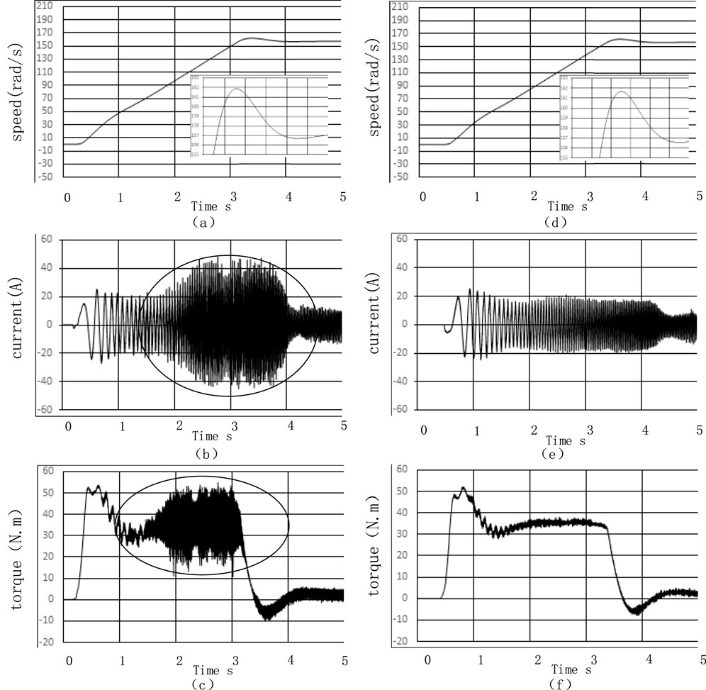
Figure 9. Simulation waveforms of no-load starting to 50 Hz (a) Motor speed waveform of conventional vector control algorithm (b) Current waveform of conventional vector control algorithm (c) Electromagnetic torque waveform of conventional vector control algorithm (d) Motor speed waveform of proposed vector control algorithm (e) Current waveform of proposed vector control algorithm (f) Electromagnetic torque waveform of proposed vector control algorithm.

Figure 10

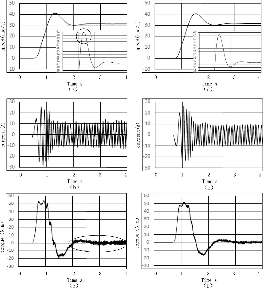
Figure 10. Simulation waveforms of no-load startup to 10 Hz (a) Motor speed waveform of conventional vector control algorithm (b) Current waveform of conventional vector control algorithm (c) Electromagnetic torque waveform of conventional vector control algorithm (d) Motor speed waveform of proposed vector control algorithm (e) Current waveform of proposed vector control algorithm (f) Electromagnetic torque waveform of proposed vector control algorithm.

Figure 11

Figure 11. Simulation waveforms of no-load speed regulation from 50 Hz to 10 Hz (a) Motor speed waveform of conventional vector control algorithm (b) Current waveform of conventional vector control algorithm (c) Electromagnetic torque waveform of conventional vector control algorithm (d) Motor speed waveform of the proposed vector control algorithm (e) Current waveform of the proposed vector control algorithm (f) Electromagnetic torque waveform of the proposed vector control algorithm.

Figure 12

Figure 12. Simulation waveforms of rated load starting to 50 Hz (a) Motor speed waveform with conventional vector control algorithm (b) Current waveform with conventional vector control algorithm (c) Electromagnetic torque waveform with conventional vector control algorithm (d) Motor speed waveform with proposed vector control algorithm (e) Current waveform with proposed vector control algorithm (f) Electromagnetic torque waveform with proposed vector control algorithm.

Figure 13

Figure 13. Simulation waveforms of rated load starting to 10 Hz (a) Motor speed waveform with conventional vector control algorithm (b) Current waveform with conventional vector control algorithm (c) Electromagnetic torque waveform with conventional vector control algorithm (d) Motor speed waveform with the proposed vector control algorithm (e) Current waveform with the proposed vector control algorithm (f) Electromagnetic torque waveform with the proposed vector control algorithm.

Figure 14

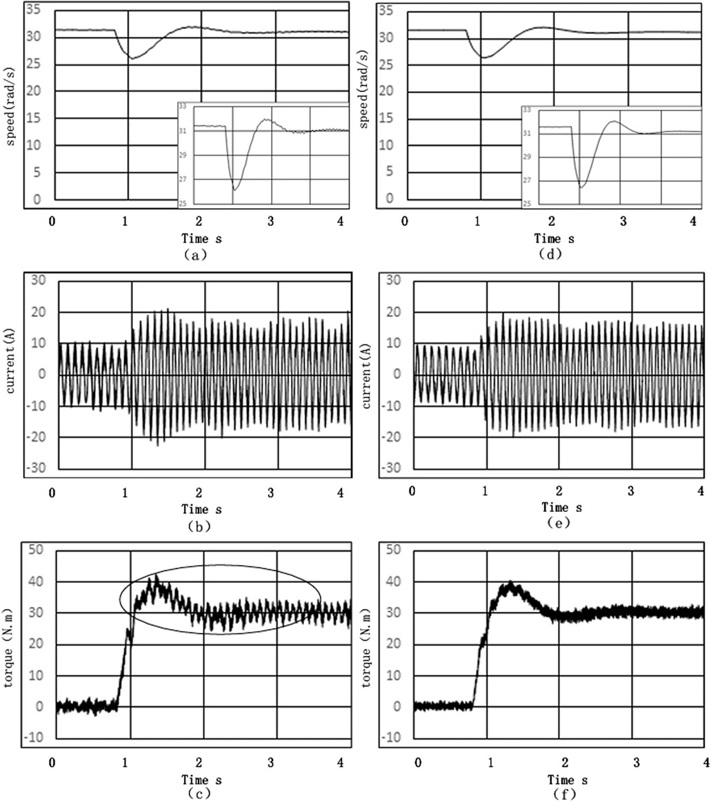
Figure 14. Simulation sudden load response at 10 Hz waveforms (a) Motor speed waveform with conventional vector control algorithm (b) Current waveform with conventional vector control algorithm (c) Electromagnetic torque waveform with conventional vector control algorithm (d) Motor speed waveform with the proposed vector control algorithm (e) Current waveform with the proposed vector control algorithm (f) Electromagnetic torque waveform with the proposed vector control algorithm.

Figure 15

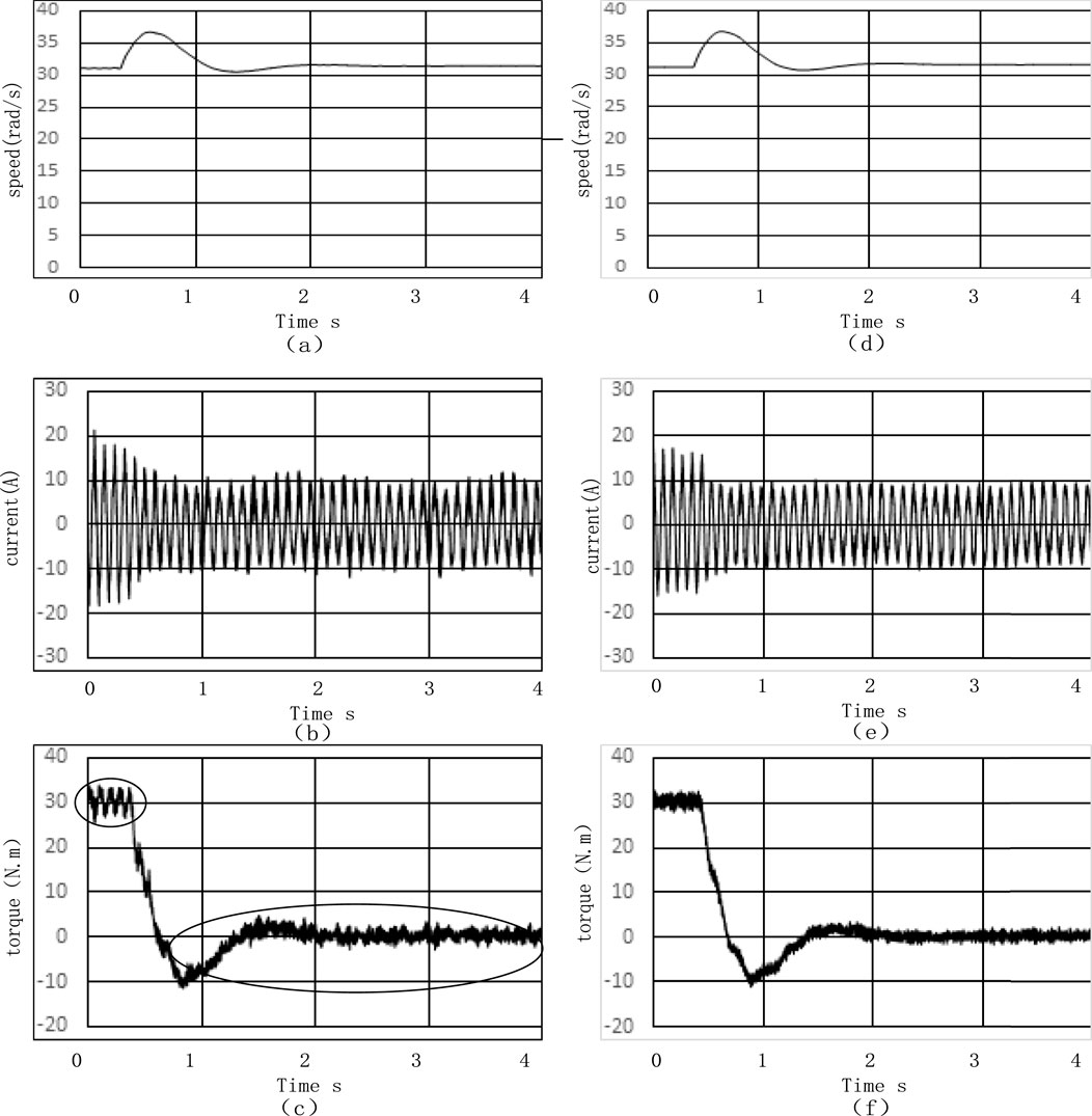
Figure 15. Simulation sudden unload response at 10 Hz waveforms (a) Motor speed waveform based on conventional vector control algorithm (b) Current waveform based on conventional vector control algorithm (c) Electromagnetic torque waveform based on conventional vector control algorithm (d) Motor speed waveform based on improved vector control algorithm (e) Current waveform based on improved vector control algorithm (f) Electromagnetic torque waveform based on improved vector control algorithm.

Figure 16

Figure 16. The simulation no-load start-up to 50 Hz waveforms, when introducing time-varying parameters (a) Motor speed waveform of the conventional vector control algorithm (b) Current waveform of the conventional vector control algorithm (c) Electromagnetic torque waveform of the conventional vector control algorithm (d) Motor speed waveform of the proposed vector control algorithm (e) Current waveform of the proposed vector control algorithm (f) Electromagnetic torque waveform of the proposed vector control algorithm.

4.1 Simulation analysis

4.1.1 Simulation parameters

The main circuit model used in this paper is a three-phase inverter with a DC power supply of 600 V. The specific parameters of the simulation models are: Table 2 lists the parameters of this long cable model, resistivity is 0.34 $\mathrm{\Omega }/\text{km}$, distributed inductance is 0.38 $\text{mH}/\text{km}$, distributed capacitance is 0.29 $\mu \mathrm{F}/\text{km}$. As shown in Tables 4, 5, The inductance of the filter model is 2.25 mH, the capacitance of the filter model is 1 $\mu \mathrm{F}$, induction motor’s rated power, number of pole pairs, rated voltage, rated current, rated frequency, rated speed, stator resistance, rotor resistance, mutual inductance, rotor leakage inductance, stator leakage inductance are 5.5 $\text{kW}$, 2, AC380 V, 11.6 A, 50 Hz, 1440 rpm, 1.1 $\mathrm{\Omega }$, 0.666 $\mathrm{\Omega }$, 164.8 mH, 4.75 mH, 4.75 mH, respectively.

Table 2

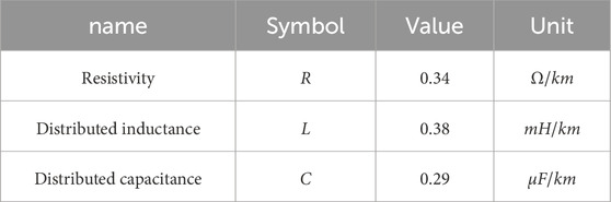
Table 2. Long cable parameters (1 km).

Table 3

Table 3. Filter parameters.

Table 4

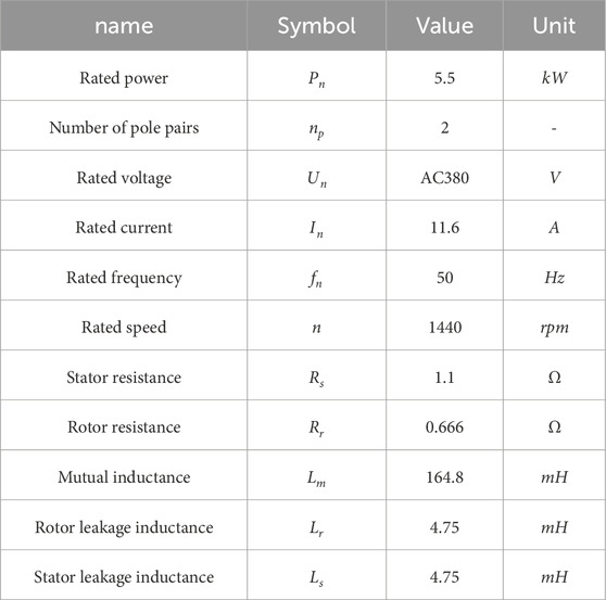
Table 4. Induction motor parameters.

4.1.2 The simulation results under various operating conditions at different frequencies and analysis

As shown in Figure 9, these are the simulation waveforms from no-load startup to 50 Hz. The left side shows the simulations with the original control algorithm, while the right side displays the simulations with the improved control algorithm. The motor successfully started at 4 s, the rotational speed reached 150 rad/s, the current stabilized, and finally settled at a peak value range of $\pm$ 10 A (Root Mean Square (RMS) value is 7.07 A); the torque reached 50 N·m at the moment of startup. From waveforms (c), (d), (e), and (f), it can be observed that during the startup process, the original vector control algorithm exhibits significant current fluctuation (areas circled in the diagram), which could cause overheating in the induction motor if left unaddressed. The improved algorithm has essentially eliminated the current fluctuation. The original algorithm also shows substantial torque fluctuation (areas circled in the diagram), it is between 50 N·m and 20 N·m, and the improved control algorithm is stable at about 35 N m, the torque fluctuation is reduced by about 15 N·m. Other advanced control methods, such as optimizing pole-slot fit, can reduce torque fluctuation at no-load startup by 35 %–40%, and oblique pole design can reduce torque fluctuation at no-load startup by 45 %–50%; however, these methods are not applied to the condition of long cables.

As shown in Figure 10, the simulation waveforms depict the no-load startup to 10 Hz, where the current reached a peak value range of $\pm$ 10 A (RMS value is 7.07 A), the rotational speed reached 30 rad/s, and the induction motor successfully started after 3 s. The improved control algorithm achieves a more stable torque after 2 s.

As shown in Figure 11, the simulation waveforms illustrate the no-load speed adjustment from 50 Hz to 10 Hz, with the induction motor successfully starting by 2.8 s, the rotational speed dropped to 35 rad/s, the current stabilized, and finally settled at a peak value range of $\pm$ 10 A (RMS value is 7.07 A). The torque fluctuation of the improved control algorithm is reduced.

As shown in Figure 12, the simulation waveforms illustrate the motor starting under rated load up to 50 Hz. The motor successfully started within 4 s, the rotational speed reached 155 rad/s, the current stabilized, and finally settled at a peak value range of $\pm$ 15 A (RMS value is 10.6 A). By comparing (c), (d), (e), and (f), it can be observed that the pre-improvement vector control algorithm exhibits significant fluctuations in current and torque (highlighted in circled areas) due to the influence of parasitic impedance, inductive reactance, and capacitive reactance in long cables. Without intervention, this would cause the induction motor to overheat. In contrast, the improved control algorithm demonstrates greater stability in current and torque during startup, reduces spikes, and better adapts to oscillation disturbances in long-cable environments, thereby preventing motor overheating.

As shown in Figure 13, the simulation waveforms depict the induction motor starting under rated load up to 10 Hz, the rotational speed has reached 30 rad/s, the current stabilized, and finally settled at a peak value range of $\pm$ 20 A (RMS value is 14.14 A). The induction motor successfully started within 2 s with reduced torque ripple. The improved control algorithm achieves constant torque startup.

Figure 14 shows the simulation waveforms of sudden load response at 10 Hz. With the stator rotational speed remaining at 30 rad/s overall, there were certain fluctuations within 2 s. The current stabilized at a peak value range of ±20 A (RMS value is 14.14 A). The torque reached approximately 40 N·m and then stabilized at around 30 N·m. The improved algorithm reduces the torque fluctuations.

As shown in Figure 15, it is the simulation waveforms of sudden unload. On the premise that the overall rotational speed remains unchanged, which was 30 rad/s, there were certain fluctuations within 2 s. The current stabilized at a peak value range of ±10 A (RMS value is 7.07 A). The torque reached 30 N·m at the moment of startup. The improved control algorithm lessens the torque fluctuation.

4.1.3 Simulation results of No-Load startup to 50 Hz with time-varying parameters introduced and analysis

Figure 16 shows the simulation of no-load start-up to 50 Hz waveforms, when introducing time-varying parameters, the long cable’s R, L, and C increase by 0.017 $\mathrm{\Omega }$, 0.019 mH, and 0.0145 $\mu \mathrm{F}$, respectively.

It can be seen from the simulation waveforms that the improved algorithm can adapt to the changes brought about by 5% increase in parameters of the long cable under the no-load startup condition, which is basically consistent with the waveforms in Figure 9. The current was initially between a peak value range of ±20 A (RMS value is 14.14 A), and then stabilized at a peak value range of ±10 A (RMS value is 7.07 A). The waveforms before improvement show more dense fluctuations in current and torque in the area circled by the circle.

4.2 Experimental Analysis

As shown in Figure 17, an experimental platform for the improved vector control algorithm was set up in the laboratory to verify whether the improved algorithm can enhance the response characteristics. The experimental platform consists of a motor test unit, a long cable model, a VFD, and a sine wave filter.

Figure 17

Figure 17. Experimental platform of the improved vector control algorithm.

4.2.1 Experimental parameters

The rated power of the induction motor is 5.5 kW. It is a motor with 2 pole pairs. The rated voltage is AC 380 V, the rated current is 11.6 A, and the rated frequency is 50 Hz. The rated speed is 1440 rpm. The stator resistance is 1.1 $\mathrm{\Omega }$, the rotor resistance is 0.666 $\mathrm{\Omega }$, the mutual inductance is 164.8 mH, the rotor leakage inductance is 4.75 mH, and the stator leakage inductance is 4.75 mH. A long cable (1 km) is used, which has a resistance of 0.34 $\mathrm{\Omega }$, an inductance of 0.38 mH, and a capacitance of 0.29 $\mu \mathrm{F}$. A customized VFD is used in the experiment. The filter uses an inductance of 2.25 mH and a capacitance of 1 $\mu \mathrm{F}$. The bandwidth of the oscilloscope is 750 MHz, and the sampling rate is 4 GSa/s. The peak voltage of the 100 MHz high-voltage differential probe is 1500 V, the attenuation settings are 500X or 50X, the bandwidth settings are FULL (full bandwidth) or 5 MHz, and the output impedance is 1 MΩ. The bandwidth of the low-voltage probe is 200 MHz, the impedance is 1 MΩ, and the input capacitance is 3.5 pF. The conversion ratio of the current probe is 0.01 V/A at the 500 A range and 0.1 V/A at the 75 A range. The force-sensitive amplifier, as part of the measurement system, processes the signals from the torque sensor and speed sensor. The measurement range of torque is 0–100 N·m, and the output signal corresponding to the full-scale range is 0–20 mA. The measurement range of speed is 0–2000 rpm, and the output signal corresponding to the full-scale range is 0–20 mA.

4.2.2 Experimental results and analysis

As shown in Figures 18–23, the experimental waveforms of the conventional and improved vector control algorithm display current (blue), torque (red), and speed (yellow).

Figure 18

Figure 18. Experimental waveforms of no-load startup for the conventional vector control algorithm.

Figure 19

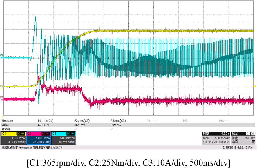
Figure 19. Experimental waveforms of no-load startup for the improved vector control algorithm.

Figure 20

Figure 20. Experimental waveforms of the conventional vector control algorithm during sudden load.

Figure 21

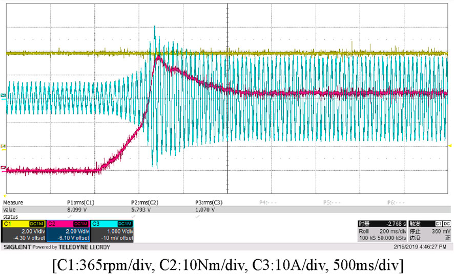
Figure 21. Experimental waveforms of the improved vector control algorithm during sudden load.

Figure 22

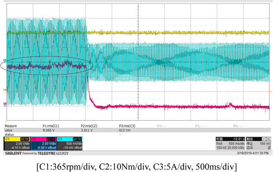
Figure 22. Experimental waveforms of the conventional control algorithm during sudden unload.

Figure 23

Figure 23. Experimental waveforms of the improved vector control algorithm during sudden unload.

From Figures 18, 19, corresponding to the simulation in Figure 9, the following can be observed: During no-load startup, the actual rotational speed reaches 152.89 rad/s (1460 rpm), while the simulated value is 150 rad/s. The actual current finally stabilizes at around a peak value range of ±11 A (RMS value is 7.78 A), and the simulated peak value range is ±10 A (RMS value is 7.07 A). At the moment of startup, the actual torque reaches 45 N·m, while the simulated value is 50 N·m. When the conventional control algorithm is adopted during the no-load startup process of the motor, the electromagnetic torque vibration (the circled area) has certain fluctuations, causing certain fluctuations in the current. In contrast, the proposed control algorithm increases the starting electromagnetic torque of the motor and improves its operating performance.

From Figures 20, 21, corresponding to the simulation in Figure 14, we can see: During sudden load application, the actual rotational speed reaches 152.89 rad/s (1460 rpm), whereas the simulated value is 30 rad/s, since the simulation frequency is 10 Hz, the rotational speed is equal to 2π times the frequency and divided by the number of pole pairs, the frequency of 50 Hz is five times that of 10 Hz, the number of pole pairs of the motor in the simulation is the same as that in the experiment, the rotational speed corresponding to 50 Hz is 150 rad/s, which is consistent with the experimental results. The actual current finally stabilizes at around a peak value range of ±20 A (RMS value is 14.14 A), consistent with the simulated value range. At the moment of startup, the actual torque reaches around 45 N·m, while the simulated value is around 40 N·m. Using the conventional control algorithm, when a sudden load is applied during the motor’s operation, the electromagnetic torque is close to 45 N·m (the circled area). This increases the speed recovery time, leads to a decrease in the operating speed, and makes it difficult to restore the speed to the given reference speed. However, when the proposed control algorithm is used and the same load is suddenly applied during the motor’s operation, the electromagnetic torque is close to 47 N·m. It increases the operating torque of the motor, reduces the pulsation of the electromagnetic torque, and enables the motor’s operating speed to quickly recover to the given reference speed after the sudden load application.

From Figures 22, 23, corresponding to the simulation in Figure 15, it can be found that: During sudden unloading, the actual rotational speed reaches 152.89 rad/s (1460 rpm), whereas the simulated value is 30 rad/s, since the simulation frequency is 10 Hz, the rotational speed is equal to 2π times the frequency and divided by the number of pole pairs, the frequency of 50 Hz is five times that of 10 Hz, the number of pole pairs of the motor in the simulation is the same as that in the experiment, the rotational speed corresponding to 50 Hz is 150 rad/s, which is consistent with the experimental results. The actual current finally stabilizes at around a peak value range of ±7 A (RMS value is 4.95 A), while the simulated value is a peak value range of ±10 A (RMS value is 7.07 A). At the moment of startup, the actual torque reaches 30 N·m, which is the same as the simulated value range 30 N·m. When the conventional control algorithm is used, sudden unloading during the motor’s rated-load operation causes fluctuations in the motor torque (the circled area) and makes it difficult to restore the speed to the given reference speed. The proposed control algorithm can reduce the pulsation of the electromagnetic torque and enable the motor to quickly recover to the given operating speed.

4.3 FFT simulation results and analysis

As shown in Table 5 and Figures 24–29, FFT simulations were conducted for 10 Hz no-load operating, 30 Hz no-load operating, and 50 Hz no-load operating. The THD of the 10 Hz FFT was 8.28% before improvement and 5.41% after improvement. The THD of 30 Hz was 7.70% before improvement and 4.45% after improvement. The THD of 50 Hz was 4.41% before improvement and 4.37% after improvement. The improved control algorithm significantly reduced the THD of the operating current.

Table 5

Table 5. FFT results of the no-load motor current.

Figure 24

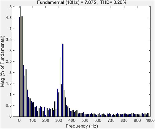
Figure 24. FFT simulation waveform of no-load operating current at 10 Hz for conventional speed sensorless vector control algorithm in the algorithm before the improved power supply system.

Figure 25

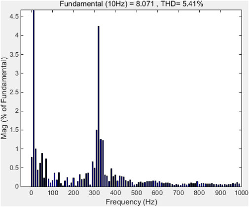
Figure 25. FFT simulation waveform of current under no-load operation at 10 Hz for the speed sensorless vector control algorithm of the improved algorithm power supply system.

Figure 26

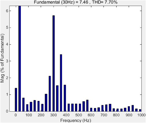
Figure 26. FFT simulation waveform of the conventional speed sensorless vector control algorithm current under no-load operation at 30 Hz in the algorithm before the improved power supply system.

Figure 27

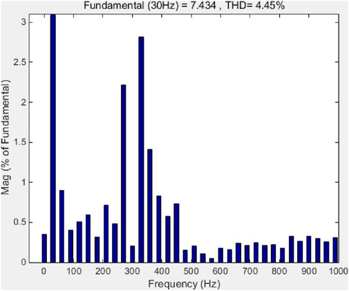
Figure 27. FFT simulation waveform of no-load operating current for the speed sensorless vector control algorithm of the improved algorithm power supply system at 30 Hz.

Figure 28

Figure 28. FFT simulation waveform of the conventional speed sensorless vector control algorithm for the algorithm before improvement, the power supply system under no-load operation at 50 Hz

Figure 29

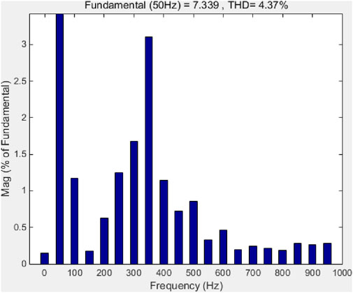
Figure 29. FFT simulation waveform of the no-speed sensor vector control algorithm current for the improved algorithm power supply system under 50 Hz no-load operation.

5 Conclusion

Aiming at the insufficient adaptability of existing vector control algorithms to filter and long cable parameters (under the influence of parasitic impedance, parasitic capacitance, and parasitic inductance), which leads to unresolved stability on no-load startup, sudden-load startup, and harmonic issues, this paper proposes a sensorless vector control algorithm based on Lyapunov theory. By establishing the full-system transfer function of the filter-cable-motor, we provide the proof of asymptotic stability. The FFT simulation results show that: THD during 10 Hz no-load operating decreases from 8.28% to 5.41%, 30 Hz from 7.70% to 4.45%, while 50 Hz no-load operating shows 0.04% THD degradation. The improved algorithm demonstrates certain adaptability to time-sensitivity parameters and improves the torque and current response of the induction motor. Experimental verifications on no-load startup, sudden load, and sudden unload were carried out. Compared with previous studies, this paper overcomes the limitations of missing stability theory and provides a more reliable control solution for deep-sea long-cable motor drives. In detail:

Through calculations, torque and flux linkage errors are determined, and the error transfer function is formulated, followed by a stability proof. The results demonstrate that the stability constant is greater than zero, indicating the system is asymptotically stable.

Also, this paper quantitatively analyzes the impacts of various time-dependent conditions of deep-sea long cables on cable parameters, added it to the proposed long cable model, and the Lyapunov function is used to prove its stability, to further analyze the proposed function’s stability, this paper introduced long cable health model, proof equations were proposed and conducted analysis, proposed that operation maintenance and replace the long cables when they reach the end of their service life can effectively address the issues that the time-dependent variations of deep-sea long cable parameters pose to the method presented in this paper.

At last, future work will focus on applications in deep-sea oil extraction and further improve the simulations and experiments.

Data availability statement

The original contributions presented in the study are included in the article/supplementary material, further inquiries can be directed to the corresponding authors.

Author contributions

ZJ: Writing – original draft, Writing – review and editing, Validation, Software. YD: Validation, Writing – original draft, Software, Writing – review and editing.

Funding

The author(s) declare that no financial support was received for the research and/or publication of this article.

Acknowledgments

The authors would like to thank all the reviewers for their useful revisions, which improved the quality of the paper.

Conflict of interest

The authors declare that the research was conducted in the absence of any commercial or financial relationships that could be construed as a potential conflict of interest.

Generative AI statement

The author(s) declare that no Generative AI was used in the creation of this manuscript.

Any alternative text (alt text) provided alongside figures in this article has been generated by Frontiers with the support of artificial intelligence and reasonable efforts have been made to ensure accuracy, including review by the authors wherever possible. If you identify any issues, please contact us.

Publisher’s note

All claims expressed in this article are solely those of the authors and do not necessarily represent those of their affiliated organizations, or those of the publisher, the editors and the reviewers. Any product that may be evaluated in this article, or claim that may be made by its manufacturer, is not guaranteed or endorsed by the publisher.

References

Adamczyk, M., and Orlowska-Kowalska, T. (2024). Current sensor fault-tolerant control based on modified luenberger observers for safety-critical vector-controlled induction motor drives. Bull. Pol. Acad. Sci. Tech. Sci. 72 (5). doi:10.24425/bpasts.2024.151041

CrossRef Full Text | Google Scholar

Avery, P. (2023). How to get the most from your variable frequency drive. Control Eng. 70 (4), 34–36.

Google Scholar

Bonczar, R. (2022). Set up, tune a PM motor, VFD. Control Eng. 69 (2), 32–33.

Google Scholar

Boukhili, F., Zaafouri, A., and Dami, M. A. (2022). 3-Phase induction motor speed control based space vector modulation technique for direct matrix converter under unbalanced conditions. J. Electr. Syst. 18 (2), 246–259.

Google Scholar

Callegari, J. M. S., Vitoi, L. A., and Brandao, D. I. (2023). VFD-based coordinated multi-stage centralized/decentralized control to support offshore electrical power systems. IEEE Trans. Smart Grid 14 (4), 2863–2873. doi:10.1109/TSG.2022.3224616

CrossRef Full Text | Google Scholar

Chien, C. H., and Bucknall, R. W. G. (2007). Analysis of harmonics in subsea power transmission cables used in VSC-HVDC transmission systems operating under steady-state conditions. IEEE Trans. Power Deliv. 22 (4), 2489–2497. doi:10.1109/TPWRD.2007.905277

CrossRef Full Text | Google Scholar

Das, A., and Chatterjee, S. (2025). A novel speed sensor-less stator flux-oriented vector control of dual-stator induction generator for grid-tied wind energy conversion system. Int. J. Circuit Theory Appl. 53 (1), 380–408. doi:10.1002/cta.4070

CrossRef Full Text | Google Scholar

Deng, Y., Liang, Z., Xia, P., and Zuo, X. (2019). Improved speed sensorless vector control algorithm of induction motor based on long cable. J. Electr. Eng. & Technol. 14, 219–229. doi:10.1007/s42835-018-00023-7

CrossRef Full Text | Google Scholar

Dursun, M. (2023). Fitness distance balance-based runge–kutta algorithm for indirect rotor field-oriented vector control of three-phase induction motor. Neural Comput. Appl. 35 (18), 13685–13707. doi:10.1007/s00521-023-08408-0

CrossRef Full Text | Google Scholar

Feng, F., Hu, H., Ge, Q., Yang, J., and Cheng, L. (2024). Speed sensorless vector control of linear induction motors based on fuzzy extended kalman filter. J. Railw. Sci. Eng. 21 (3), 1168–1179. doi:10.19713/j.cnki.43-1423/u.T20230666

CrossRef Full Text | Google Scholar

Hasan, F. (2025). Vector control of the induction motor based on whale optimization algorithm. Int. J. Electr. Comput. Eng. Syst. 16 (1), 31–37. doi:10.32985/ijeces.16.1.4

CrossRef Full Text | Google Scholar

Lekhchine, S., Bahi, T., and Soufi, Y. (2014). Indirect rotor field oriented control based on fuzzy logic controlled double star induction machine. Int. J. Electr. Power Energy Syst. 57, 206–211. doi:10.1016/j.ijepes.2013.11.053

CrossRef Full Text | Google Scholar

Liang, X., Kar, N. C., and Liu, J. (2014). Load filter design method for medium-voltage drive applications in electrical submersible pump systems. IEEE Trans. Industry Appl. 51 (3), 2017–2029. doi:10.1109/TIA.2014.2369814

CrossRef Full Text | Google Scholar

Liang, X., He, J., and Du, L. (2015). Electrical submersible pump system grounding: current practice and future trend. IEEE Trans. Industry Appl. 51 (6), 5030–5037. doi:10.1109/TIA.2015.2432096

CrossRef Full Text | Google Scholar

Liu, Z., Ren, D., Chen, J., Zhang, K., Yang, Y., and Wang, F. (2025). Study of SVPWM control algorithm with voltage balancing based on simplified vector for cascaded H-bridge energy storage converters. Electr. Eng. 107 (2), 1411–1425. doi:10.1007/s00202-024-02595-2

CrossRef Full Text | Google Scholar

Qiao, S., Huang, J., Xu, Y., and Song, K. (2025). Direct model predictive torque control for permanent magnet synchronous motor with voltage vector parallel optimisation algorithm. IET Electr. Power Appl. 19 (1), e70007. doi:10.1049/elp2.70007

CrossRef Full Text | Google Scholar

Qin, G., Liu, M., Zou, J., and Xin, X. (2015). Vector control algorithm for electric vehicle AC induction motor based on improved variable gain PID controller. Math. Problems Eng. 2015, 1–9. doi:10.1155/2015/875843

CrossRef Full Text | Google Scholar

Rahman, M. I., and Salim, K. M. (2019). Performance evaluation of single-phase induction motor controlled by variable frequency drive at non-ideal voltage conditions. Aust. J. Electr. Electron. Eng. 16 (2), 65–73. doi:10.1080/1448837X.2019.1600213

CrossRef Full Text | Google Scholar

Singh, G., and Naikan, V. N. A. (2018). Detection of half broken rotor bar fault in VFD driven induction motor drive using motor square current MUSIC analysis. Mech. Syst. Signal Process. 110, 333–348. doi:10.1016/j.ymssp.2018.03.001

CrossRef Full Text | Google Scholar

Smochek, M., Pollice, A. F., Rastogi, M., and Harshman, M. (2016). Long cable applications from a medium-voltage drives perspective. IEEE Trans. industry Appl. 52 (1), 645–652. doi:10.1109/TIA.2015.2463760

CrossRef Full Text | Google Scholar

Sprovieri, J. (2014). Applying VFDs to servo applications: AC induction motors are increasingly being used in applications once dominated by servomotors. Assembly 57 (7).

Google Scholar

Tao, R., Jiang, Y., and Wang, W. (2024). “Super-twisting algorithm sliding mode observer-based multi-vector model-free predictive control method for PMSM,” in 2024 27th International Conference on Electrical Machines and Systems, ICEMS 2024, 864–869. doi:10.23919/ICEMS60997.2024.10921251

CrossRef Full Text | Google Scholar

Xia, P., Liang, Z., and Zuo, X. (2018). Fractional-order modeling and starting voltage drop analysis of long-distance variable frequency drive systems for electric submersible pumps in deep-sea oilfields. Petroleum Sci. Bull. 04, 452–465.

Google Scholar

Yao, Y. (2002). Optimization design and condition diagnosis of submersible electric pump production systems in offshore oilfields. Chengdu: Southwest Petroleum Institute.

Google Scholar

Yaseen, F. R., and Al-Khazraji, H. (2025). Optimized vector control using swarm bipolar algorithm for five-level PWM inverter-fed three-phase induction motor. Int. J. Robotics Control Syst. 5 (1), 333–347. doi:10.31763/ijrcs.v5i1.1713

CrossRef Full Text | Google Scholar

Zhang, A. 'an, Yuan, H., Wang, Y., and Qian, Li (2025). A time-varying comprehensive state evaluation model for submarine cables considering environmental impacts. High. Volt. Appar. 61 (07), 189–196. doi:10.13296/j.1001-1609.hva.2025.07.022

CrossRef Full Text | Google Scholar

Zhu, H., Du, J., and Liu, G. (2024). Decoupling control of bearingless permanent magnet synchronous motor based on least squares support vector machine inverse system optimized by improved grey wolf optimization algorithm. Prog. Electromagn. Res. C 141, 109–121. doi:10.2528/PIERC23122301

CrossRef Full Text | Google Scholar