Improving the synchronous stability of grid-following converters using flux linkage feedback combined with the DFF neural network

A hybrid scheme of flux linkage feedback (FLF) combined with the deep feed-forward (DFF)-genetic algorithm (GA) method to improve the synchronous stability of grid-following (GFL) converters is proposed in this paper. By subtracting three-phase flux linkages from three-phase voltage references generated by the GFL controller, the FLF and the parameter optimization based on DFF-GA are expected to improve the equivalent virtual damping in the dynamics of the angular speed of the phase-locked loop (PLL). The implementation of the proposed method will reduce the risk of synchronous instability of the converter with respect to the stability region. The virtual flux linkages can be calculated by the integration of the instantaneous voltage; thus, no additional measurement is required. The effectiveness of FLF has been verified by region of attraction, simulation, and experimental studies, which show that the system with the FLF scheme presents longer critical clearing time (CCT) than the traditional method and the PLL damping enhancement strategy. Moreover, the proposed scheme does not change the internal structure of the existing controller and is easy to implement on various GFL converters.

1 Introduction

The generation of renewable energy sources such as wind power and solar power has grown at an unprecedented rate in the past decade. As the interface between renewable energy sources and the grid, grid-following (GFL) converters are widely used in renewable power connection and high-voltage direct-current (HVDC) transmission (Wang et al., 2022). Owing to the ability of transmitting large-scale power with a simple implementation method, the GFL converter has been an indispensable component of renewable energy generation (Wang et al., 2022; Aljarrah et al., 2024). The GFL converter based on the PI controller of the inner and outer control loops exhibits “low inertia and weak damping,” which indicates weak synchronous stability capability (Chen X. et al., 2024). When a large disturbance occurs, the GFL converter is prone to be unstable due to the instability of the phase-locked loop (PLL). Thus, it is necessary to enhance the equivalent damping of the GFL converter.

The GFL converter measures the angle and angular frequency of grid voltage using the PLL, whose stability depends on the strength of the external grid. For enhancing its synchronous stability, the existing strategies can be classified into three forms: regulating the active power reference during fault, equipping the DC chopper, and improving equivalent damping. In the study by Taul et al. (2019), the active power reference value is decreased to increase the deceleration area during the fault. Li X. et al. (2023) proposed a dynamic active current regulation method to improve the synchronous stability of GFL converters. Furthermore, an adaptive active power reference value controller according to the voltage dynamics during fault, which can improve the recovery ability of the converter, was designed by Ma et al. (2018). For restraining the active power overshoot at the time of the large disturbance, Naderi et al. (2019) designed a DC chopper to dissipate the excess power generated during a brief time of fault. An integrated dissipation equipment that combines the advantages of a voltage source converter (VSC) and a DC chopper was introduced by Wu et al. (2022). The implementation of the chopper can resist the power overshoot at the moment of the large disturbance, but it cannot essentially improve the damping characteristics of the converter. A fault ride-through control strategy without a DC chopper was proposed by Badar et al. (2023), in which active power during fault is regulated by controlling the capacitor voltage of the converter. However, this method is limited by the dynamic characteristics of the capacitor.

Considering that equivalent damping is closely related to the synchronous stability of GFL converters, it is feasible to improve the equivalent damping. In studies by Li et al. (2024) and Li et al. (2023b), the PI controller parameters of the PLL can be enhanced through a deep learning approach to improve the equivalent damping of GFL converters. Huang and Vanfretti (2023) proposed an adaptive damping control method for GFL converters. Adaptive damping is calculated by voltage and current, and finally fed into the modulator. However, the adaptive damping method proposed by Huang and Vanfretti (2023) aimed to suppress high-frequency oscillations, and its effect toward transient stability has not been studied. Furthermore, Sun et al. (2024) introduced additional damping into the PLL based on the expression of power-angle characteristics to improve the transient stability of the converter. In addition, the PI controller parameters of the PLL are also the factors affecting the synchronous stability of the GFL converter. In the study by Wang et al. (2020), the PI parameters of the PLL are real-time adjusted under large disturbances, but this strategy is difficult to apply practically due to the short transient time during the fault. A constant damping is introduced in the PLL through the feedback of angular frequency (Li et al., 2025). To increase the equivalent damping, a PI controller feedback loop is introduced in parallel with the original PI controller of the PLL (Huang et al., 2022). In the study by Liu et al. (2021), a transient damping loop achieved by different voltage sags is added behind the PI controller of the PLL, which can adaptively adjust the converter’s damping ratio for different voltage sags. However, the existing transient stability enhancement method through optimizing the PLL is still complex and difficult to be implemented. Furthermore, the effectiveness of enhancing the equivalent damping by regulating the PLL structure is limited because it involves matching the PLL parameters.

For the transient stability analysis of converters, the existing methods can be divided into three forms: electromagnetic simulation, power-angle analysis, and region of attraction (ROA) (Liu et al., 2025; Chen L. et al., 2024). Electromagnetic simulation is widely used in transient stability analysis due to its advantages such as simple implementation and intuitive results (Chen X. et al., 2024). The power-angle analysis is mainly applied to the stability analysis of single-machine models (Xiahou et al., 2025). However, for multi-machine large-scale systems, due to their complex structure and difficulties in modeling, it is difficult to apply the above two methods for analysis. Therefore, scholars have proposed the method of ROA to estimate the large-scale systems (Liu et al., 2024). However, as the system complexity escalates, existing ROA estimate methods face multifaceted limitations. For addressing the above problems, the sum of squares (SOS) programming method is proposed by Izumi (2018) to estimate the ROA.

Inspired by the control structure in the study by Huang and Vanfretti (2023), a FLF scheme is proposed in this paper without changing the original structure of the PLL to enhance the equivalent damping combined with parameter optimization using the deep feed-forward (DFF)-genetic algorithm (GA). The main contributions of the proposed method and work in this paper can be summarized as follows:

• Based on second-order differential equations, the dynamic response of the PLL is derived and analyzed.

•The FLF strategy is proposed based on the dynamic response of the PLL for enhancing the virtual equivalent damping.

•For further improving the synchronous stability of the GFL converter, a DFF-GA-based PLL parameter optimization strategy is also designed.

In summary, the paper is structured as follows. Section 2 introduces the design of the FLF scheme and DFF-GA-based parameter optimization algorithm. The dynamic model based on second-order differential equations of the system with and without FLF scheme is established in Section 3. The comparisons of ROA using the SOS programming method, comparative simulation results, and experiment results are given in Section 4. Based on the results of the time-domain simulation and experiments, conclusions are drawn in Section 5.

2 Design of the hybrid control scheme

2.1 Flux linkage feedback in the grid-following control system

The three-phase converter considered here has a constant power input $P_{\text{in}}$, which is modeled by connecting a controlled current source in parallel to the DC-side capacitor, with the output current being $P_{\text{in}}/V_{\text{dc}}$, as shown in Figure 1. $R_{\text{f}}$ and $L_{\text{f}}$ are the filter resistance and filter impedance, respectively. $R_{\text{g}}$ and $L_{\text{g}}$ are the gird resistance and gird impedance, respectively. ${\bar{V}}_{\text{d}1}$, ${\bar{V}}_{\text{q}1}$, ${\bar{i}}_{\text{d}1}$, and ${\bar{i}}_{\text{q}1}$ are the per unit value output current and voltage of the converter in the dq-frame. The grid-following control is realized in the dq reference frame. The d-axis control loop is used to regulate the capacitor voltage $V_{\mathrm{d}\mathrm{c}}$, and the q-axis control loop is used to regulate the reactive power output $Q$ of the converter. A PLL is used to capture the phase angle and angular frequency of the voltage vector $\vec{v}$ of the filter capacitors $C_{\mathrm{f}}$. The phase angle output ${\theta }_{\text{pll}}$ of the PLL is used as the phase angle input of the Park transformation to generate the dq components of three-phase voltages and currents, and it is also used as the phase angle reference to generate the three-phase reference voltages for the converter, that is, ${\bar{e}*}_{\mathrm{a}}$, ${\bar{e}*}_{\mathrm{b}}$, and ${\bar{e}*}_{\mathrm{c}}$.

Figure 1

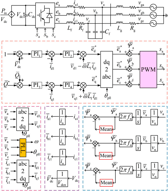
Figure 1. Schematic of a grid-following control system with FLF of a three-phase converter system ($(\bar{\cdot })$ denotes the per unit value of a variable).

Inspired by the control block in the study by Huang and Vanfretti (2023), the structure of the FLF for the GFL controller is also presented in Figure 1. The FLF is realized by subtracting the three-phase flux linkages ${\bar{\mathrm{\Psi }}}_{\mathrm{a}}$, ${\bar{\mathrm{\Psi }}}_{\mathrm{b}}$, and ${\bar{\mathrm{\Psi }}}_{\mathrm{c}}$ of the filter capacitor node from the three-phase reference voltages generated by the current loop. The obtained three-phase signals are used as the inputs of the pulse width modulation (PWM) block, using which triggering pulses $s_{\mathrm{a}}$, $s_{\mathrm{b}}$, and $s_{\mathrm{c}}$ are generated for converter bridges. If overmodulation does not occur, the following are the three-phase output voltages of the converter:

${\bar{e}}_{\mathrm{a}}={\bar{e}}_{\mathrm{a}}^{*}-{\bar{\mathrm{\Psi }}}_{\mathrm{a}},{\bar{e}}_{\mathrm{b}}={\bar{e}}_{\mathrm{b}}^{*}-{\bar{\mathrm{\Psi }}}_{\mathrm{b}},{\bar{e}}_{\mathrm{c}}={\bar{e}}_{\mathrm{c}}^{*}-{\bar{\mathrm{\Psi }}}_{\mathrm{c}}.(1)$

The three-phase flux linkages of the filter capacitor node are calculated by Equation 2.

$\left\{\begin{array}{cc}\hfill & {\bar{\mathrm{\Psi }}}_{\mathrm{a}}={\bar{\mathrm{\Psi }}}_{\mathrm{a}}^{\prime }-\mathrm{M}\mathrm{e}\mathrm{a}\mathrm{n}\left({\bar{\mathrm{\Psi }}}_{\mathrm{a}}^{\prime }\right)\hfill \\ \hfill & {\bar{\mathrm{\Psi }}}_{\mathrm{b}}={\bar{\mathrm{\Psi }}}_{\mathrm{b}}^{\prime }-\mathrm{M}\mathrm{e}\mathrm{a}\mathrm{n}\left({\bar{\mathrm{\Psi }}}_{\mathrm{b}}^{\prime }\right)\hfill \\ \hfill & {\bar{\mathrm{\Psi }}}_{\mathrm{c}}={\bar{\mathrm{\Psi }}}_{\mathrm{c}}^{\prime }-\mathrm{M}\mathrm{e}\mathrm{a}\mathrm{n}\left({\bar{\mathrm{\Psi }}}_{\mathrm{c}}^{\prime }\right)\hfill \end{array}\right.(2)$

where

$p{\bar{\mathrm{\Psi }}}_{\mathrm{a}}^{\prime }=2\pi f_{\mathrm{n}}{v}_{\mathrm{a}}/v_{\text{n}},p{\bar{\mathrm{\Psi }}}_{\mathrm{b}}^{\prime }=2\pi f_{\mathrm{n}}{v}_{\mathrm{b}}/v_{\text{n}},p{\bar{\mathrm{\Psi }}}_{\mathrm{c}}^{\prime }=2\pi f_{\mathrm{n}}{v}_{\mathrm{c}}/v_{\text{n}},(3)$

where $p=d/dt$ in Equation 3 represents the differential operator, $\mathrm{M}\mathrm{e}\mathrm{a}\mathrm{n}(\cdot )$ represents the mean value of a variable over a period of $1/f_{\mathrm{n}}$, the $\mathrm{M}\mathrm{e}\mathrm{a}\mathrm{n}$ block is to eliminate the asymmetric component of single-phase flux linkages, $f_{\mathrm{n}}$ is the rated frequency of the system in Hz, $v_{\mathrm{n}}$ denotes the nominal peak phase-to-ground voltage in V, and $v_{\mathrm{a}}$, $v_{\mathrm{b}}$, and $v_{\mathrm{c}}$ are the three-phase voltages of the filter capacitor node.

Applying Clark transformation on the two sides of Equations 3, 4, we obtain

$p\left[\begin{array}{c}\hfill {\bar{\mathrm{\Psi }}}_x^{\prime }\hfill \\ \hfill {\bar{\mathrm{\Psi }}}_y^{\prime }\hfill \end{array}\right]=2\pi f_{\mathrm{n}}\left[\begin{array}{c}\hfill {\bar{v}}_x\hfill \\ \hfill {\bar{v}}_y\hfill \end{array}\right],(4)$

where the zero sequence components are neglected as the symmetrical three-phase circuit is considered here. The vector of node flux linkage can be written as $\stackrel{⃗}{{\bar{\mathrm{\Psi }}}^{\prime }}={\bar{\mathrm{\Psi }}}_x^{\prime }+j{\bar{\mathrm{\Psi }}}_y^{\prime }$, and the vector of node voltage can be denoted as $\overrightarrow{\stackrel{̄}{v}}={\bar{v}}_x+j{\bar{v}}_y$. The vector form of Equation 4 can be written as $p\stackrel{⃗}{{\bar{\mathrm{\Psi }}}^{\prime }}=2\pi f_{\mathrm{n}}\overrightarrow{\stackrel{̄}{v}}$. By writing the vectors in the polar coordinate form, we have $\stackrel{⃗}{{\bar{\mathrm{\Psi }}}^{\prime }}={\bar{\mathrm{\Psi }}}^{\prime }{\mathrm{e}}^{j{\theta }_{\bar{\mathrm{\Psi }}}}$, $\overrightarrow{\stackrel{̄}{v}}=\bar{v}{\mathrm{e}}^{j{\theta }_{\bar{v}}}$, and Equation 5 can be obtained as

$\left[p{\bar{\mathrm{\Psi }}}^{\prime }+j{\bar{\mathrm{\Psi }}}^{\prime }p{\theta }_{\bar{\mathrm{\Psi }}}\right]{\mathrm{e}}^{j{\theta }_{\bar{\mathrm{\Psi }}}}=2\pi f_{\mathrm{n}}\bar{v}{\mathrm{e}}^{j{\theta }_{\bar{v}}}.(5)$

In the steady state, the magnitude and angular frequency of sinusoidal signals remain constant, that is, $p{\bar{\mathrm{\Psi }}}^{\prime }=0$ and $p{\theta }_{\bar{\mathrm{\Psi }}}={\omega }_{\bar{\mathrm{\Psi }}}$. Therefore, the steady-state relationship between the voltage and flux linkage vectors can be described by Equation 6.

${\bar{\mathrm{\Psi }}}^{\prime }=\bar{v},{\theta }_{\bar{\mathrm{\Psi }}}+\frac{\pi }{2}={\theta }_{\bar{v}},\overrightarrow{\stackrel{̄}{v}}=j{\overrightarrow{\stackrel{̄}{\mathrm{\Psi }}}}^{\prime },(6)$

where ${\bar{\omega }}_{\bar{\mathrm{\Psi }}}={\omega }_{\bar{\mathrm{\Psi }}}/(2\pi f_{\mathrm{n}})=1$. Magnitudes of the per unit flux linkage and voltage vectors are the same, and the flux linkage vector leads the node voltage vector by 90$°$ in the steady state.

2.2 Parameter optimization for the PLL using DFF-GA

According to Ma et al. (2022), parameters of the PLL have a significant impact on the synchronous stability of GFL converters. Taking advantage of the data-driven technique, a DFF neural network is employed to study the nonlinear expression of the overshoot and the stabilization time of system frequency in terms of PLL parameters, and the GA is used to search for the optimal solution of this expression to obtain the optimal parameters for the PLL. The DFF-GA-based parameter optimization for the PLL is constructed as shown in Figure 2. $f_{\text{s}}$ and $t_{\text{s}}$ denote the overshoot and settling time of the system frequency, respectively, where $Cos{t}_{\text{train}}=2.4f_{\text{s}}+1.2t_{\text{s}}$. $K_{\text{pop}}$ and $K_{\text{iop}}$ are the optimal parameters with DFf-GA. A total of 10,000 sets of data are randomly divided into 8,000 sets of the training set and 2,000 sets of the test set, which are obtained by the Simulink model. The input data are the proportional–integral (PI) parameters of the PLL shown in Figure 5. Each input layer of the DFF is expressed by Equation 7.

$o_i^{\left(l\right)}\left(n\right)=\left\{\begin{array}{cc}\hfill & x_i\left(n\right),l=1\hfill \\ \hfill & f\left(P_j^{\left(l-1\right)}\left(n\right)+b^{\left(l-1\right)}\left(n\right)\right),l=\mathrm{2,3,4}\hfill \end{array}\right.(7)$

Here, $x_i(n)$ indicates the input of the DFF; $x_1=K_{\text{p}}$ and $x_2=K_{\text{i}}$, $n=1,\dots ,8000$, and $f(\cdot )$ represent the transfer function of the hidden layer, for example, $f(x)=max(0,x)$; and $l$ denotes the layer number of the DFF. The output of each layer is defined as Equation 8.

$P_j^{\left(l\right)}\left(n\right)={\displaystyle \sum _{i=1}^q}{W}_{i,j}^{\left(l\right)}\left(n\right)o_i^{\left(l\right)}\left(n\right)l=\mathrm{1,2,3,4}.(8)$

Figure 2

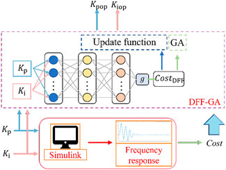
Figure 2. Schematic of the DFF-GA-based parameter optimization for the PLL.

The output of DFF is expressed as Equation 9.

$Cos{t}_{\text{DFN}}=g\left(P_j^{\left(l\right)}\left(n\right)+b_n^{\left(l\right)}\right),l=4,(9)$

where $g(x)=x$, and the values of $i,j,q$ can be obtained in Table 1.

Table 1

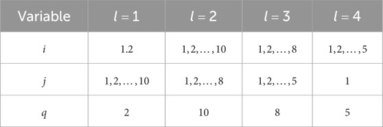
Table 1. Value of $i,j,q$.

The performance index function is expressed by the quadratic error function as Equation 10.

$L\left(n\right)=\frac{1}{2}{\left[Cos{t}_{\text{train}}\left(n\right)-Cos{t}_{\text{DFN}}\left(n\right)\right]}^2.(10)$

The weight $W_{i,j}^{(l)}(n)$ and bias $b^{(l)}(n)$ update functions are performed using the gradient descent method as Equation 11.

$\begin{array}{cc}\hfill & W_{i,j}^{\left(l\right)}\left(n+1\right)=W_{i,j}^{\left(l\right)}\left(n\right)-\eta \frac{\partial L\left(n\right)}{\partial W_{i,j}^{\left(l\right)}\left(n\right)}\hfill \\ \hfill & b^{\left(l\right)}\left(n+1\right)=b^{\left(l\right)}\left(n\right)-\eta \frac{\partial L\left(n\right)}{\partial b^{\left(l\right)}\left(n\right)}\hfill \end{array},(11)$

where $\eta$ denotes the network learning rate, and $\eta =0.01$. GA is equipped to solve the global minimum value of the obtained nonlinear function. With the advantages of excellent global search capabilities, outstanding adaptability to nonlinear objective functions, and universality, the GA is utilized to search the optimal solution, which includes the process of selection, crossover, and mutation, and its process is shown in Figure 3.

Figure 3

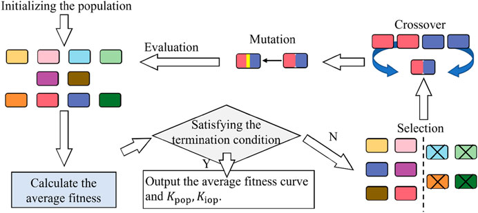
Figure 3. Scheme of the GA process.

3 Analytical comparisons of synchronous stability of GFL converters with and without FLF

For the converter system shown in Figure 1, the spatial relationship of different reference frames and voltage vectors is as illustrated in Figure 4. ${\theta }_{\mathrm{f}}$ denotes the phase angle of $\vec{v}$ in the abc stationary reference frame, and $\theta$ is the phase angle of $\vec{v}$ in the synchronously rotating xy reference frame. $\omega$ denotes the angular speed of the dq reference frame generated by the PLL in rad/s, and ${\omega }_{\mathrm{n}}=2\pi f_{\mathrm{n}}$ is the rated angular speed of the system in rad/s. The following assumptions are made in the synchronous stability modeling and analysis:

• $\vec{v}$ rotates at the rated angular speed ${\omega }_{\mathrm{n}}$.

•The x-axis is aligned with the a-axis at $t=0$s; that is, ${\theta }_{\mathrm{f}}(0)=\theta$.

•The phase angle of ${\vec{v}}_{\mathrm{g}}$ is zero; that is, ${\vec{v}}_{\text{g}}=v_{\text{g}}$.

•${\bar{R}}_{\mathrm{f}}\ll {\bar{X}}_{\mathrm{f}}$, ${\bar{R}}_{\mathrm{g}}\ll {\bar{X}}_{\mathrm{g}}$, ${\bar{X}}_{\mathrm{f}}={\bar{L}}_{\mathrm{f}}$, and ${\bar{X}}_{\mathrm{g}}={\bar{L}}_{\mathrm{g}}$.

Figure 4

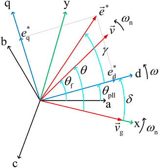
Figure 4. Spatial relationship of different reference frames and voltage vectors.

The above assumptions can be found in most studies on the synchronous stability of GFL converters (Ma et al., 2022; Li and Du, 2022).

The schematic of the PLL is as illustrated in Figure 5. The angle between the x-axis and d-axis is defined as $\delta$, which can be written as $\delta ={\theta }_{\mathrm{p}\mathrm{l}\mathrm{l}}+\theta -{\theta }_{\mathrm{f}}$. According to assumption A2, it has ${\theta }_{\mathrm{f}}=\theta +2\pi f_{\mathrm{n}}t$, and thus, $\delta ={\theta }_{\mathrm{p}\mathrm{l}\mathrm{l}}-2\pi f_{\mathrm{n}}t$. According to Ma et al. (2022) and Hu et al. (2019), the dynamics of $\delta$ is used to describe the synchronous stability of grid-following converter, i.e., as shown in Equation 12.

$\left\{\begin{array}{cc}\hfill & p\delta =2\pi f_{\mathrm{n}}\mathrm{\Delta }\bar{\omega }\hfill \\ \hfill & p\mathrm{\Delta }\bar{\omega }=K_{\mathrm{i}}{\bar{v}}_{\mathrm{q}\mathrm{1}}+K_{\mathrm{p}}p{\bar{v}}_{\mathrm{q}\mathrm{1}}\hfill \end{array}\right.(12)$

Here, $K_{\mathrm{p}}$ and $K_{\mathrm{i}}$ are the proportional and integral coefficients of the PI controller, respectively.

Figure 5

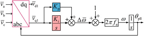
Figure 5. Schematic of the phase-locked loop.

For the grid-following control without FLF, it has ${\bar{e}}_{\text{a}}={\bar{e}*}_{\text{a}}$, ${\bar{e}}_{\text{b}}={\bar{e}*}_{\text{b}}$, ${\bar{e}}_{\text{c}}={\bar{e}*}_{\text{c}}$, and also the vector form $\vec{e}=\vec{e}*$. The x-axis and y-axis components of $\overrightarrow{\stackrel{̄}{v}}$ can be obtained as Equation 13.

$\begin{array}{cc}\hfill & {\bar{v}}_{\text{x}}=\frac{{\bar{X}}_{\text{f}}}{{\bar{X}}_{\text{f}}+{\bar{X}}_{\text{g}}}{\bar{v}}_{\text{g}}+\frac{{\bar{X}}_{\text{g}}}{{\bar{X}}_{\text{f}}+{\bar{X}}_{\text{g}}}\bar{e}\mathrm{c}\mathrm{o}\mathrm{s}\left(\delta +\gamma \right)\hfill \\ \hfill & {\bar{v}}_{\text{y}}=\frac{{\bar{X}}_{\text{g}}}{{\bar{X}}_{\text{f}}+{\bar{X}}_{\text{g}}}\bar{e}\mathrm{s}\mathrm{i}\mathrm{n}\left(\delta +\gamma \right)\hfill \end{array},(13)$

where $\gamma$ is the angle of vector $\overrightarrow{\stackrel{̄}{e}}*$ in the dq reference frame, as shown in Figure 4. As ${\bar{v}}_{\text{q}1}={\bar{v}}_{\text{y}}\mathrm{c}\mathrm{o}\mathrm{s}\delta -{\bar{v}}_{\text{x}}\mathrm{s}\mathrm{i}\mathrm{n}\delta$, the Equation 14 is obtained.

$p{\bar{v}}_{\text{q}1}=-\frac{{\bar{X}}_{\text{f}}}{{\bar{X}}_{\text{f}}+{\bar{X}}_{\text{g}}}{\bar{v}}_{\text{g}}\mathrm{c}\mathrm{o}\mathrm{s}\delta \mathrm{\Delta }\omega +\frac{{\bar{X}}_{\text{g}}}{{\bar{X}}_{\text{f}}+{\bar{X}}_{\text{g}}}\left(p\bar{e}\mathrm{s}\mathrm{i}\mathrm{n}\gamma +\bar{e}p\gamma \mathrm{c}\mathrm{o}\mathrm{s}\gamma \right).(14)$

With Equation 14, the second equation of Equation 12 can be written as Equation 15.

$\begin{array}{cc}\hfill p\mathrm{\Delta }\bar{\omega }& =\frac{{\bar{X}}_{\text{f}}}{{\bar{X}}_{\text{f}}+{\bar{X}}_{\text{g}}}\left[K_{\text{i}}\bar{e}\mathrm{s}\mathrm{i}\mathrm{n}\gamma {\bar{X}}_{\text{g}}/{\bar{X}}_{\text{f}}-K_{\text{i}}{\bar{v}}_{\text{g}}\mathrm{s}\mathrm{i}\mathrm{n}\delta \right.\hfill \\ \hfill & \left.{- K}_{\text{p}}{\bar{v}}_{\text{g}}\mathrm{c}\mathrm{o}\mathrm{s}\delta \mathrm{\Delta }\omega +K_{\text{p}}\left(p\bar{e}\mathrm{s}\mathrm{i}\mathrm{n}\gamma +\bar{e}p\gamma \mathrm{c}\mathrm{o}\mathrm{s}\gamma \right){\bar{X}}_{\text{g}}/{\bar{X}}_{\text{f}}\right]\hfill \end{array}.(15)$

For the grid-following control with FLF, it has $\overrightarrow{\stackrel{̄}{e}}=\overrightarrow{\stackrel{̄}{e}}*-\overrightarrow{\stackrel{̄}{\mathrm{\Psi }}}$, which is according to Equation 1. The x-axis and y-axis components of $\overrightarrow{\stackrel{̄}{v}}$ can be obtained as Equation 16.

$\begin{array}{cc}\hfill & {\bar{v}}_{\text{x}}=\frac{{\bar{v}}_{\text{g}}{\bar{X}}_{\text{f}}\left({\bar{X}}_{\text{f}}+{\bar{X}}_{\text{g}}\right)}{{\bar{X}}_{\text{g}}^2+{\left({\bar{X}}_{\text{f}}+{\bar{X}}_{\text{g}}\right)}^2}\hfill \\ \hfill & + \frac{\bar{e}{\bar{X}}_{\text{g}}}{{\bar{X}}_{\text{g}}^2+{\left({\bar{X}}_{\text{f}}+{\bar{X}}_{\text{g}}\right)}^2}\left[\left({\bar{X}}_{\text{f}}+{\bar{X}}_{\text{g}}\right)\mathrm{c}\mathrm{o}\mathrm{s}\left(\delta +\gamma \right)-{\bar{X}}_{\text{g}}\mathrm{s}\mathrm{i}\mathrm{n}\left(\delta +\gamma \right)\right]\hfill \\ \hfill & {\bar{v}}_{\text{y}}=\frac{{\bar{v}}_{\text{g}}{\bar{X}}_{\text{f}}{\bar{X}}_{\text{g}}}{{\bar{X}}_{\text{g}}^2+{\left({\bar{X}}_{\text{f}}+{\bar{X}}_{\text{g}}\right)}^2}\hfill \\ \hfill & + \frac{\bar{e}{\bar{X}}_{\text{g}}}{{\bar{X}}_{\text{g}}^2+{\left({\bar{X}}_{\text{f}}+{\bar{X}}_{\text{g}}\right)}^2}\left[{\bar{X}}_{\text{g}}\mathrm{c}\mathrm{o}\mathrm{s}\left(\delta +\gamma \right)+\left({\bar{X}}_{\text{f}}+{\bar{X}}_{\text{g}}\right)\mathrm{s}\mathrm{i}\mathrm{n}\left(\delta +\gamma \right)\right]\hfill \end{array}.(16)$

The expression of ${\bar{v}}_{\text{q}1}$ can be obtained by substituting Equation 16 into ${\bar{v}}_{\text{q}1}={\bar{v}}_{\text{y}}\mathrm{c}\mathrm{o}\mathrm{s}\delta -{\bar{v}}_{\text{x}}\mathrm{s}\mathrm{i}\mathrm{n}\delta$. The expression of $d{\bar{v}}_{\text{q}1}/dt$ is obtained as Equation 17.

$\begin{array}{cc}\hfill p{\bar{v}}_{\text{q}1}& =-\frac{{\bar{X}}_{\text{f}}}{\sqrt{{\bar{X}}_{\text{g}}^2+{\left({\bar{X}}_{\text{f}}+{\bar{X}}_{\text{g}}\right)}^2}}{\bar{v}}_{\text{g}}\mathrm{c}\mathrm{o}\mathrm{s}\left(\delta -\tau \right)\mathrm{\Delta }\omega \hfill \\ \hfill & + \frac{{\bar{X}}_{\text{g}}}{\sqrt{{\bar{X}}_{\text{g}}^2+{\left({\bar{X}}_{\text{f}}+{\bar{X}}_{\text{g}}\right)}^2}}\left[p\bar{e}\mathrm{s}\mathrm{i}\mathrm{n}\left(\gamma +\tau \right)+\bar{e}p\gamma \mathrm{c}\mathrm{o}\mathrm{s}\left(\gamma +\tau \right)\right],\hfill \end{array}(17)$

where $\tau =\mathrm{a}\mathrm{t}\mathrm{a}\mathrm{n}[{\bar{X}}_{\text{g}}/({\bar{X}}_{\text{f}}+{\bar{X}}_{\text{g}})]$. With Equation 17, the second equation of Equation 12 can be written as Equation 18

$\begin{array}{cc}\hfill p\mathrm{\Delta }\bar{\omega }=& \frac{{\bar{X}}_{\text{f}}}{\sqrt{{\bar{X}}_{\text{g}}^2+{\left({\bar{X}}_{\text{f}}+{\bar{X}}_{\text{g}}\right)}^2}}\left\{K_{\text{i}}\bar{e}\mathrm{s}\mathrm{i}\mathrm{n}\left(\gamma +\tau \right){\bar{X}}_{\text{g}}/{\bar{X}}_{\text{f}}\right.\hfill \\ \hfill & -K_{\text{i}}{\bar{v}}_{\text{g}}\mathrm{s}\mathrm{i}\mathrm{n}\left(\delta -\tau \right)-K_{\text{p}}{\bar{v}}_{\text{g}}\mathrm{c}\mathrm{o}\mathrm{s}\left(\delta -\tau \right)\mathrm{\Delta }\omega \hfill \\ \hfill & +\left.K_{\text{p}}\left[p\bar{e}\mathrm{s}\mathrm{i}\mathrm{n}\left(\gamma +\tau \right)+\bar{e}p\gamma \mathrm{c}\mathrm{o}\mathrm{s}\left(\gamma +\tau \right)\right]{\bar{X}}_{\text{g}}/{\bar{X}}_{\text{f}}\right\}.\hfill \end{array}(18)$

By comparing Equation 15 and Equation 18, the following two observations are obtained.

•The equivalent time constant of the dynamics of the angular speed deviation $\mathrm{\Delta }\bar{\omega }$ is increased by FLF due to $\sqrt{{\bar{X}}_{\text{g}}^2+{({\bar{X}}_{\text{f}}+{\bar{X}}_{\text{g}})}^2}>{\bar{X}}_{\text{f}}+{\bar{X}}_{\text{g}}$.

•The damping coefficient, which is the coefficient of $\mathrm{\Delta }\omega$ in the right-hand side of the two equations, is increased from $K_{\text{p}}{\bar{v}}_{\text{g}}\mathrm{c}\mathrm{o}\mathrm{s}\delta$ to $K_{\text{p}}{\bar{v}}_{\text{g}}\mathrm{c}\mathrm{o}\mathrm{s}(\delta -\tau )$ by FLF, on the condition that ${\bar{X}}_{\text{g}}$ is small in strong AC grids such that $|\delta -\tau |<\delta$.

Because of the higher time constant and damping coefficient, the FLF is expected to improve the synchronous stability of the GFL converter. The time constant mentioned above is usually regarded as the equivalent inertia constant of the converter as well.

4 Simulation and experiment studies

4.1 Region of attraction results

In order to validate the theoretical observations above, the exact ROA and estimated ROA are investigated. For acquiring the exact ROA, time-domain simulation is implemented to determine whether the collected operating point is a stable equilibrium point. For acquiring the estimated ROA, the Lyapunov function and its level set have to be searched by adding the coordinate transformation of the equality constraints into Equation 15 and Equation 18, and then solving the following SOS programming problem which are divided into Equations 19, 20, 22, 23. The coordinate transformation can be described as ${\mathit{z}}_{(2i-1)}=sin{\theta }_{\text{pll}},{\mathit{z}}_{(2i)}=1-cos{\theta }_{\text{pll}}$.

$\begin{array}{c}\mathbf{S}\mathbf{O}\mathbf{S}\mathbf{P}\mathbf{0}\mathbf{a}:\underset{V,s_1\in {\mathrm{\Sigma }}_{\mathrm{M}}\left[\mathit{z}\right],V\left(0\right)=0,{\lambda }_1,{\lambda }_2\in {\mathbb{P}}_{\mathrm{M}}\left[\mathit{z}\right]}{\text{search}}V\hfill \\ \mathrm{s}.\mathrm{t}.\hfill \\ V-{{\lambda }_1}^{\top }\mathrm{G}-q_1\in {\mathrm{\Sigma }}_{\mathrm{M}}\left[\mathit{z}\right]\hfill \\ -s_1\left(\beta -p\right)-\dot{V}-{{\lambda }_2}^{\top }\mathrm{G}-q_2\in {\mathrm{\Sigma }}_{\mathrm{M}}\left[\mathit{z}\right]\hfill \end{array},(19)$

where $q_1(\mathit{z})={ϵ}_1{\left|\left|\mathit{z}\right|\right|}_2^2$ and $q_2(\mathit{z})={ϵ}_2{\left|\left|\mathit{z}\right|\right|}_2^2$, and ${ϵ}_{\mathrm{1,2}}$ indicate small positive real numbers. $\mathrm{G}$ denotes the vector established by equality constraints. After a feasible $V(\mathit{z})$ is found and rewritten as $V_{0a}(\mathit{z})$, it is necessary to search for a maximum level set satisfying ${\dot{V}}_{0a}(\mathit{z})<0$ to hold $\bigvee \mathit{z}\in V_{0a}^{\gamma }(\mathit{z})/0$, which can be achieved by solving the following SOS programming problem.

$\begin{array}{c}\mathbf{S}\mathbf{O}\mathbf{S}\mathbf{P}\mathbf{0}\mathbf{b}:\underset{s_2,s_3\in {\mathrm{\Sigma }}_{\mathrm{M}}\left[\mathit{z}\right],{\lambda }_2\in {\mathbb{P}}_{\mathrm{M}}\left[\mathit{z}\right]}{\max }\gamma \hfill \\ \mathrm{s}.\mathrm{t}.\hfill \\ -s_2\left(\gamma -V_{0\mathrm{a}}\right)-s_3{\dot{V}}_{0\mathrm{a}}-{\lambda }_2^{\top }\mathrm{G}-q_1\in {\mathrm{\Sigma }}_{\mathrm{M}}\left[\mathit{z}\right]\hfill \end{array}.(20)$

As the $-s_2\gamma$ in SOSP0b is a bilinear term, it should be solved by a bisection search on $\gamma$ to gain the optimal solution ${\gamma }_{0b}$. Then, a new function $V_{\text{0b}}(\mathit{z})=V_{0a}(\mathit{z})/{\gamma }_{0b}$ can also be regarded as an initial Lyapunov function for Equation 15 and Equation 18. In order to obtain the largest estimated ROA of the state equation, an iterative searching for $V(\mathit{z})$ is implemented by the following SOS programming program.

$\begin{array}{c}\mathbf{S}\mathbf{O}\mathbf{S}\mathbf{P}\mathbf{1}:\underset{\genfrac{}{}{0pt}{}{V_1^{\left(i+1\right)},s_4,s_5,s_6\in {\mathrm{\Sigma }}_{\mathrm{M}}\left[\mathit{z}\right],V_1^{\left(i+1\right)}\left(0\right)=0,}{{\lambda }_3,{\lambda }_4,{\lambda }_5\in {\mathbb{P}}_{\mathrm{M}}\left[\mathit{z}\right]}}{\text{search}}{V}_1^{\left(i+1\right)}\hfill \\ \mathrm{s}.\mathrm{t}.\hfill \\ -s_4\left(1-V_1^{\left(i\right)}\right)+\left(1-V_1^{\left(i+1\right)}\right)-{\lambda }_3^{\top }\mathrm{G}\in {\mathrm{\Sigma }}_{\mathrm{M}}\left[\mathit{z}\right]\hfill \\ V_1^{\left(i+1\right)}-{\lambda }_4^{\top }\mathrm{G}-q_1\in {\mathrm{\Sigma }}_{\mathrm{M}}\left[\mathit{z}\right]\hfill \\ -s_5\left(1-V_1^{\left(i+1\right)}\right)-s_6{\dot{V}}_1^{\left(i+1\right)}-{\lambda }_5^{\top }\mathrm{G}-q_2\in {\mathrm{\Sigma }}_{\mathrm{M}}\left[\mathit{z}\right]\hfill \end{array},(21)$

where $i=\mathrm{0,1,2}\dots$, and the initial Lyapunov function is set as $V_1^0(\mathit{z})=V_{0b}(\mathit{z})$. $s_1,s_2,\dots ,s_6$ denote the SOS polynomials. ${\lambda }_1,{\lambda }_2,\dots ,{\lambda }_5$ denote polynomials. Moreover, the bilinear terms in SOSP1 are $s_5{V}_1^{i+1}$ and $s_6{\dot{V}}_1^{(i+1)}$, and a coordinate-wise iterative method is employed here. Then, SOSP1 is transformed into a linear semi-definite programming problem at each iteration. Thus, SOSP1 can be realized by solving the two SOS programming problems given below.

$\begin{array}{c}\mathbf{S}\mathbf{O}\mathbf{S}\mathbf{P}\mathbf{1}\mathbf{a}:\underset{s_5\in {\mathrm{\Sigma }}_{\mathrm{M}}\left[\mathit{z}\right],{\lambda }_5\in {\mathbb{P}}_{\mathrm{M}}\left[\mathit{z}\right]}{\text{search}}{s}_5,s_6\hfill \\ \mathrm{s}.\mathrm{t}.\hfill \\ -s_5\left(1-V_1^{\left(i\right)}\right)-s_6{\dot{V}}_1^{\left(i\right)}-{\lambda }_5^{\top }\mathrm{G}-q_2\in {\mathrm{\Sigma }}_{\mathrm{M}}\left[\mathit{z}\right]\hfill \end{array}.(22)$

If the satisfied $s_5$ and $s_6$ are found and rewritten as $s_{5(1a)}$ and $s_{6(1a)}$, the second problem is written as

$\begin{array}{c}\mathbf{S}\mathbf{O}\mathbf{S}\mathbf{P}\mathbf{1}\mathbf{b}:\underset{V_1^{\left(i+1\right)}\in {\mathrm{\Sigma }}_{\mathrm{M}}\left[\mathit{z}\right],V_1^{\left(i+1\right)}\left(0\right)=0,{\lambda }_3,{\lambda }_4,{\lambda }_5\in {\mathbb{P}}_{\mathrm{M}}\left[\mathit{z}\right]}{\text{search}}{V}^{\left(i+1\right)}\hfill \\ \mathrm{s}.\mathrm{t}.\hfill \\ V_1^{\left(i+1\right)}-V_1^{\left(i\right)}-{\lambda }_3^{\top }\mathrm{G}\in {\mathrm{\Sigma }}_{\mathrm{M}}\left[\mathit{z}\right]\hfill \\ V_1^{\left(i+1\right)}-{\lambda }_4^{\top }\mathrm{G}-q_1\in {\mathrm{\Sigma }}_{\mathrm{M}}\left[\mathit{z}\right]\hfill \\ -s_{5\left(1a\right)}^i\left(1-V_1^{\left(i+1\right)}\right)-s_{6\left(1a\right)}{\dot{V}}_1^{\left(i+1\right)}-{\lambda }_5^{\top }\mathrm{G}-q_2\in {\mathrm{\Sigma }}_{\mathrm{M}}\left[\mathit{z}\right]\hfill \end{array}.(23)$

Through SOSP1a to SOSP1b, an expanding interior algorithm is realized, and the final optimal Lyapunov function for the state is obtained, Equation 15 and Equation 18. Thus, the exact ROA and the estimated ROA of the system with and without the FLF scheme are shown in Figure 6.

Figure 6

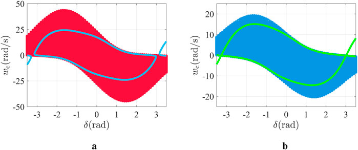
Figure 6. Exact and estimated ROA of the test system: (a) exact and estimated ROA of the GFL converter with the FLF scheme and (b) Exact and estimated ROA of the GFL converter without the FLF scheme.

In Figure 6, the exact ROA and estimated ROA of the system with the FLF scheme are larger than those of the system without the FLF scheme, which verifies the observations found in Section 3.

4.2 Simulation results

To validate the effectiveness of the FLF control and parameter optimization, simulation studies were carried out for the converter system shown in Figure 7 using MATLAB/Simulink. The control structure in Figure 7 is shown in Figure 1. The test system adopts grid-following with the FLF–DFF scheme. Two cascades of dc-linked voltage control and current control are included in the control strategy in Figure 7. The system parameters of the test system are chosen as shown in Table 2. The simulation step length was set to be $20\mu$s. The parameter optimization results by the DFF-GA method are shown in Figure 8. A three-phase-to-ground fault was applied on the PCCB at $t$ = 1s, and the simulation results under different cases are shown in Figure 9.

Figure 7

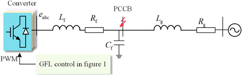
Figure 7. Topology of the test system.

Table 2

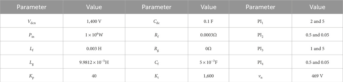
Table 2. Parameters of the GFL converter system.

Figure 8

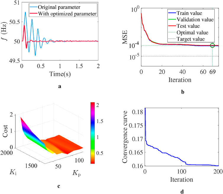
Figure 8. Performance of the DFF-GA algorithm for parameter optimization of the PLL. (a) Comparison of the system frequency dynamic response with PLL parameters before and after optimization. (b) Mean square error (MSE) of the output of DFF. (c) Convergence process of the cost function in GA optimization. (d) Convergence curve of GA.

Figure 9

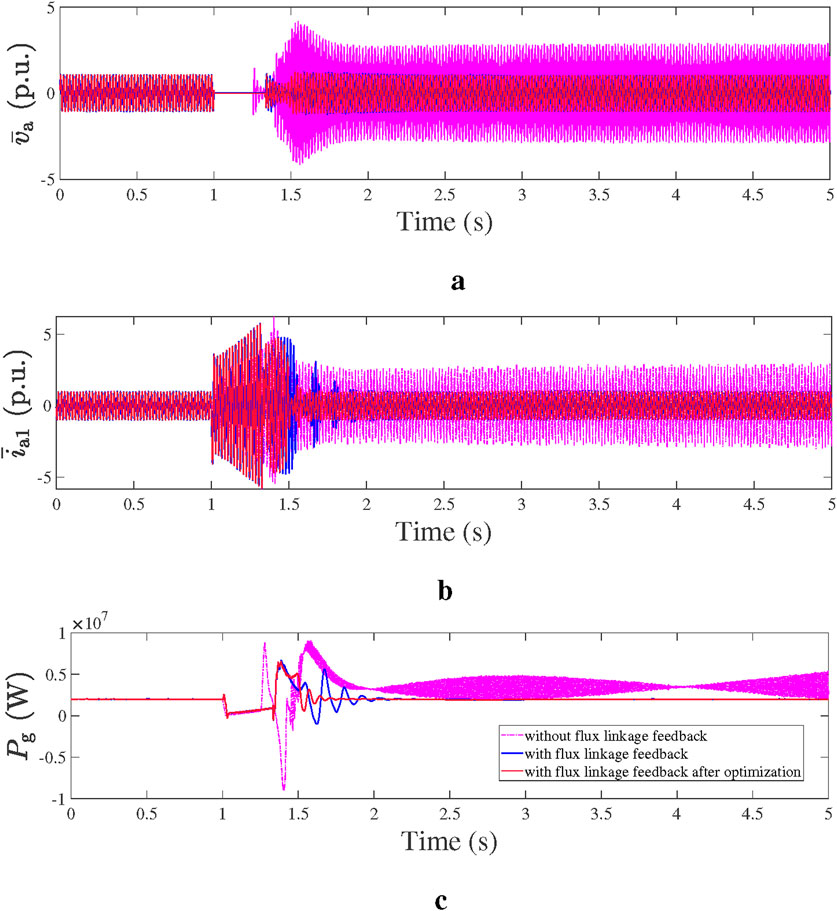
Figure 9. Performance of the grid-following converters with and without FLF, respectively. (a) A-phase voltage measured on PCCB. (b) A-phase filter current measured on the output of the converter. (c) Active power output of the GFL system.

Parameter optimization is carried out based on the system with FLF control. As shown in Figure 8b, the MSE of the output of DFF drops to $10^{-4}$, which indicates that the error between the predicted value by DFF and the real value is acceptable. The cost value of the DFF with respect to $K_{\text{p}}$ and $K_{\text{i}}$ is shown in Figure 8c; with the $K_{\text{p}}$ close to 100 and $K_{\text{i}}$ dropping to 1,500, the cost value is lower, indicating that the PLL system shows better transient response. Figure 8d shows the convergence curve of GA. When the iteration reaches to 130, the GA algorithm achieves convergence. The system with FLF after DFF-GA optimization shows the best performance. These results agree with the theoretical analysis and manifest the improved synchronous stability attributed to the FLF and DFF-GA optimization. As shown in Figure 8a, the original parameters $K_{\text{pori}}$ and $K_{\text{iori}}$ are 40 and 1,600, respectively. Through the DFF-GA optimization of the PLL parameters, the oscillation damping performance of the GFL converter has been enhanced greatly, which shows the smaller overshoot and faster transient response, where the optimal PI coefficients are obtained as $K_{\text{pop}}=88.7933$ and $K_{\text{iop}}=1411.3992$.

Figure 9 presents the results of the system with conventional PLL, conventional PLL with FLF, and conventional PLL with FLF–DFF-GA control strategies. According to the simulation results, the maximum fault clearing time of the system without FLF was 0.249 s, whereas that of the system with FLF was 0.329 s. The converter system will become unstable if the fault is not cleared within the maximum clearing time. Figure 9 shows the results of the two systems, in which the length of fault was set as 0.25 s for the one without FLF and the length of fault was set as 0.329 s for the one with FLF. According to Figure 9, the capacitor voltage, filter inductor current, and the active power output of the converter system with FLF stabilize to the pre-fault steady-state value after the 0.329 s′ fault is cleared. In contrast, the system without FLF becomes unstable after the 0.25 s′ fault is cleared. Moreover, after parameter optimization by DFF-GA, the transient stability of the system with FLF was further improved. As shown in Figure 9c, the active power of the system with FLF after DFF-GA optimization shows smaller overshoot and faster transient response than the system without FLF.

4.3 Experiment results

To compare the proposed method with the PLL damping enhancement-based method (Huang et al., 2022), the hardware-in-loop (HIL) studies are carried out. The experiments are carried out with a 2$\mathrm{M}\mathrm{W}$ three-phase grid-connected converter, whose system parameters are also shown in Table 2. The topology of the experiment system is presented in Figure 10, in which the grid-connected system is fed by RTDS. The control strategies are configured in the dSpace real-time simulator for simulation. Communication is conducted between RTDS and dSpace via optical fibers, and the simulation step size is also $20\mu$s. A three-phase-to-ground-fault was applied on PCCB at $t$ = 2 s, and the single-phase voltage and active power output results are shown in Figure 12. The strategy method scheme (Wu et al., 2022) is shown in Figure 11.

Figure 10

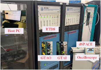
Figure 10. Topology of the experiment platform.

Figure 11

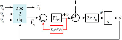
Figure 11. Topology of the PLL damping enhancement-based method.

According to the HIL results, when restrained by the control parameters of the PLL, the GFL system with PLL damping enhancement control becomes unstable when the fault clearing time (CCT) is set at 0.16 s, whereas the system with the same PLL control parameters and FLF control is larger than 0.229 s. Comparing the results in Figures 12a, b, the output active power of the system with the FLF scheme stabilizes to pre-fault steady-state values through a 0.15-s transient process after the fault is cleared. This is because of the damping coefficient introduced by the FLF strategy, which enhances the system equivalent damping. In contrast, the excess power generated by fault cannot be dissipated by the PLL damping enhancement method; this is because the equivalent damping is restricted, and then the system becomes unstable after 0.16 s′ fault is cleared. The experimental results of the system with different control schemes under three-phase-to-ground fault are presented in Table 3, which shows that the system with the hybrid scheme of FLF–DFF shows the best performance.

Figure 12

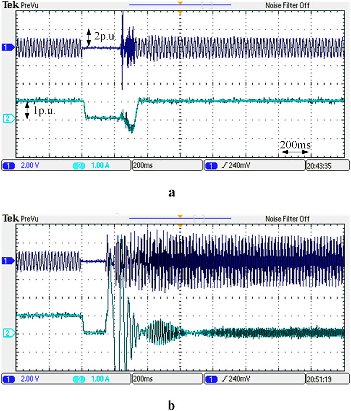
Figure 12. Experiment results of the GFL converter with different control methods. (a) Phase-A voltage of the filter capacitor and output active power of the system with FLF control. (b) Phase-A voltage of the filter capacitor and output active power of the system with PLL damping enhancement control.

Table 3

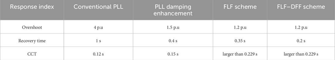
Table 3. Comparison results of the system with different control schemes.

5 Conclusion

A FLF–DFF-GA-based method is proposed in this paper for enhancing equivalent damping to improve the synchronous stability of GFL converters. The proposed method does not need to change the original structure of the PLL and is able to prolong the CCT effectively, which can be applied to the GFL converters such as the solar and wind turbine power generation systems. Apart from improving the control program, there is no need to introduce any other electrical devices either. The following conclusions are drawn from the theoretical analyses, simulations, and experiment results.

1) To overcome the limitations of enhancing equivalent damping by regulating the PLL structure, such as difficult implementation and restriction of matching PLL parameters, an FLF scheme is introduced to enhance the equivalent damping without redesigning the PLL. The analytical results based on second-order differential equations are verified by the exact and estimated ROA.

2) To further explore the damping response of the PLL, a parameter optimization method based on DFF-GA is designed. Through the training and learning of the DFF neutral network, a nonlinear expression regarding the influence of the control parameters on the dynamic response of the PLL is described. Then, a GA is designed to search the optimal parameters under the best dynamic response. Simulation results indicate that the optimization of the PLL parameters can enhance the dynamic response of GFL converters.

3) The experiment results compare the CCT of the system with the FLF scheme and with the PLL damping enhancement method, which indicate that the maximum CCT was increased by more than 32% using FLF. Moreover, the proposed method can be applied in the GFL systems of various power electronics converters without changing the PLL structure and parameter redesigning. The hybrid scheme of the current limiting strategy combined with the FLF can be taken into account for future research.

Data availability statement

The original contributions presented in this study are included in the article/Supplementary Material; further inquiries can be directed to the corresponding author.

Author contributions

YL: Writing – review and editing, Writing – original draft. HL: Methodology, Writing – original draft, Validation. YM: Writing – review and editing, Software.

Funding

The author(s) declare that no financial support was received for the research and/or publication of this article.

Conflict of interest

Author YM was employed by CSG Power Generation Co., Ltd.

The remaining authors declare that the research was conducted in the absence of any commercial or financial relationships that could be construed as a potential conflict of interest.

Generative AI statement

The author(s) declare that no Generative AI was used in the creation of this manuscript.

Publisher’s note

All claims expressed in this article are solely those of the authors and do not necessarily represent those of their affiliated organizations, or those of the publisher, the editors and the reviewers. Any product that may be evaluated in this article, or claim that may be made by its manufacturer, is not guaranteed or endorsed by the publisher.

References

Aljarrah, R., Fawaz, B. B., Salem, Q., Karimi, M., Marzooghi, H., and Azizipanah-Abarghooee, R. (2024). Issues and challenges of grid-following converters interfacing renewable energy sources in low inertia systems: a review. IEEE Access 12, 5534–5561. doi:10.1109/ACCESS.2024.3349630

CrossRef Full Text | Google Scholar

Badar, J., Akhtar, F., Kumar, D., Munir, H. M., Ali, K. H., Alsaif, F., et al. (2023). An MMC based HVDC system with optimized AC fault ride-through capability and enhanced circulating current suppression control. Front. Energy Res. 11. doi:10.3389/fenrg.2023.1190975

CrossRef Full Text | Google Scholar

Chen, L., Wen, T., Lin, Y., Liu, Y., Qin, Y., and Wu, Q.-H. (2024a). Two-stage expanding boundary algorithm to estimate domains of attraction of large-scale power systems with induction motors. IEEE Trans. Power Syst. 40, 1010–1023. doi:10.1109/TPWRS.2024.3413078

CrossRef Full Text | Google Scholar

Chen, X., Liu, Y., Wu, Q. H., Hong, C., and Su, Y. (2024b). Direct power regulation of grid-connected voltage-source inverters based on bang-bang funnel control. IEEE Trans. Industrial Electron. 71, 6460–6470. doi:10.1109/TIE.2023.3306418

CrossRef Full Text | Google Scholar

Hu, Q., Fu, L., Ma, F., and Ji, F. (2019). Large signal synchronizing instability of PLL-Based VSC connected to weak AC grid. IEEE Trans. Power Syst. 34, 3220–3229. doi:10.1109/TPWRS.2019.2892224

CrossRef Full Text | Google Scholar

Huang, S., Yao, J., Pei, J., Chen, S., Luo, Y., and Chen, Z. (2022). Transient synchronization stability improvement control strategy for grid-connected vsc under symmetrical grid fault. IEEE Trans. Power Electron. 37, 4957–4961. doi:10.1109/TPEL.2021.3131361

CrossRef Full Text | Google Scholar

Huang, P., and Vanfretti, L. (2023). Adaptive damping control of mmc to suppress high-frequency resonance. IEEE Trans. Industry Appl. 59, 7224–7237. doi:10.1109/TIA.2023.3293071

CrossRef Full Text | Google Scholar

Izumi, S., Somekawa, H., Xin, X., and Yamasaki, T. (2018). Estimation of regions of attraction of power systems by using sum of squares programming. Electr. Eng. 100, 2205–2216. doi:10.1007/s00202-018-0690-z

CrossRef Full Text | Google Scholar

Li, G., Wang, K., Liu, X., and Chen, J. (2025). A constant damping phase-locked loop for enhancing transient stability of grid-following inverter. IEEE Trans. Industrial Inf. 21, 3860–3870. doi:10.1109/TII.2025.3534430

CrossRef Full Text | Google Scholar

Li, X., Wang, Z., Zhu, L., Guo, L., and Wang, C. (2023a). Analytical dual-sequence current injections feasible region of weak-grid connected vsc under asymmetric grid faults. IEEE Trans. Power Syst. 38, 5546–5559. doi:10.1109/TPWRS.2022.3226560

CrossRef Full Text | Google Scholar

Li, Y., Ding, Y., He, S., Hu, F., Duan, J., Wen, G., et al. (2024). Artificial intelligence-based methods for renewable power system operation. Nat. Rev. Electr. Eng. 1, 163–179. doi:10.1038/s44287-024-00018-9

CrossRef Full Text | Google Scholar

Li, Y., and Du, Z. (2022). Stabilizing condition of grid-connected VSC as affected by phase locked loop (PLL). IEEE Trans. Power Deliv. 37, 1336–1339. doi:10.1109/TPWRD.2021.3115976

CrossRef Full Text | Google Scholar

Li, Y., Yu, C., Shahidehpour, M., Yang, T., Zeng, Z., and Chai, T. (2023b). Deep reinforcement learning for smart grid operations: algorithms, applications, and prospects. Proc. IEEE 111, 1055–1096. doi:10.1109/JPROC.2023.3303358

CrossRef Full Text | Google Scholar

Liu, Y., Chen, Z., Yao, H., Yi, L., and Wu, Q. H. (2024). Estimating critical clearing time of grid faults using da of state-reduction model of power systems. CSEE J. Power Energy Syst. 10, 807–820. doi:10.17775/CSEEJPES.2022.07170

CrossRef Full Text | Google Scholar

Liu, Y., Yao, H., Di, P., Qin, Y., Ma, Y., Alkahtani, M., et al. (2025). Region of attraction estimation for power systems with multiple integrated dfig-based wind turbines. IEEE Trans. Sustain. Energy, 1–15doi. doi:10.1109/TSTE.2025.3579018

CrossRef Full Text | Google Scholar

Liu, Y., Yao, J., Pei, J., Zhao, Y., Sun, P., Zeng, D., et al. (2021). Transient stability enhancement control strategy based on improved pll for grid connected vsc during severe grid fault. IEEE Trans. Energy Convers. 36, 218–229. doi:10.1109/TEC.2020.3011203

CrossRef Full Text | Google Scholar

Ma, R., Li, J., Kurths, J., Cheng, S., and Zhan, M. (2022). Generalized swing equation and transient synchronous stability with PLL-Based VSC. IEEE Trans. Energy Convers. 37, 1428–1441. doi:10.1109/TEC.2021.3137806

CrossRef Full Text | Google Scholar

Ma, S., Geng, H., Liu, L., Yang, G., and Pal, B. C. (2018). Grid-synchronization stability improvement of large scale wind farm during severe grid fault. IEEE Trans. Power Syst. 33, 216–226. doi:10.1109/TPWRS.2017.2700050

CrossRef Full Text | Google Scholar

Naderi, S. B., Negnevitsky, M., and Muttaqi, K. M. (2019). A modified dc chopper for limiting the fault current and controlling the dc-link voltage to enhance fault ride-through capability of doubly-fed induction-generator-based wind turbine. IEEE Trans. Industry Appl. 55, 2021–2032. doi:10.1109/TIA.2018.2877400

CrossRef Full Text | Google Scholar

Sun, C., Shen, K., Zhang, Y., Li, H., and Liu, Y. (2024). Rotational reference frame control of dfig-based wind turbines for inertial frequency response. IEEE Access 12, 149606–149616. doi:10.1109/ACCESS.2024.3474429

CrossRef Full Text | Google Scholar

Taul, M. G., Wang, X., Davari, P., and Blaabjerg, F. (2019). An overview of assessment methods for synchronization stability of grid-connected converters under severe symmetrical grid faults. IEEE Trans. Power Electron. 34, 9655–9670. doi:10.1109/TPEL.2019.2892142

CrossRef Full Text | Google Scholar

Wang, H., Yang, Y., Ge, X., Zuo, Y., Yue, Y., and Li, S. (2022). Pll- and fll-based speed estimation schemes for speed-sensorless control of induction motor drives: review and new attempts. IEEE Trans. Power Electron. 37, 3334–3356. doi:10.1109/TPEL.2021.3117697

CrossRef Full Text | Google Scholar

Wang, X., Taul, M. G., Wu, H., Liao, Y., Blaabjerg, F., and Harnefors, L. (2020). Grid-synchronization stability of converter-based Resources—An overview. IEEE Open J. Industry Appl. 1, 115–134. doi:10.1109/OJIA.2020.3020392

CrossRef Full Text | Google Scholar

Wu, S., Zhang, X., Jia, W., Zhu, Y., Qi, L., Guo, X., et al. (2022). A modular multilevel converter with integrated energy dissipation equipment for offshore wind vsc-hvdc system. IEEE Trans. Sustain. Energy 13, 353–362. doi:10.1109/TSTE.2021.3111751

CrossRef Full Text | Google Scholar

Xiahou, K., Du, W., Xu, X., Lin, Z., Liu, Y., Liu, Z., et al. (2025). Resilience assessment for hybrid Ac/Dc cyber-physical power systems under cascading failures. IEEE Trans. Reliab., 1–12doi. doi:10.1109/TR.2025.3550523

CrossRef Full Text | Google Scholar