Logically optimized and probabilistic integrated photovoltaic fault finding package based on machine learning

Introduction: Artificial intelligence (AI) has been widely used to detect faults and failures in photovoltaic (PV) systems, particularly those that conventional protection devices fail to identify. However, previous AI-based approaches still face major limitations, including neglecting critical detection conditions, relying on large and complex datasets, and lacking simultaneous and accurate multi-fault detection and classification.

Methods: To address these challenges, a novel PV fault detection framework is proposed by combining a fuzzy logic (FL) system with a particle swarm optimization (PSO) algorithm. An initial dataset is generated from the current–voltage (I–V) curve of a PV array. Manhattan distance (MD) and Chebyshev distance (CD) features are extracted from the I–V characteristics. A wide set of machine-learning classifiers is evaluated, and the FL system nominates the most reliable models based on mean accuracy, F1-score, and standard deviation. PSO is then used to determine the optimal subset of classifiers and to assign optimized weights for ensemble prediction. Several output-combining techniques are also examined to obtain the most accurate final classification.

Results: Model verification is performed using a dataset that includes normal operation as well as line-to-line (LL), open-circuit (OC), and degradation (DEG) faults under various environmental (irradiance, temperature) and electrical (mismatch, impedance) conditions. The proposed FL+PSO-based model achieves outstanding accuracy in detecting and classifying multiple PV faults and outperforms recent state-of-the-art approaches.

Discussion: The integration of distance-based feature extraction, fuzzy-driven classifier selection, and PSO-optimized weighting significantly enhances robustness and reduces sensitivity to environmental variations. These improvements enable reliable multi-fault detection even when fault signatures closely resemble normal conditions.

Conclusion: The proposed FL and PSO-based ensemble provides a highly accurate and reliable solution for multi-fault detection in PV arrays. Its performance surpasses existing approaches, making it a strong candidate for practical implementation in real PV monitoring systems.

1 Introduction

Photovoltaic (PV) has become a widespread source of energy throughout the world since it is clean, inexpensive, and easy to access (Ghaedi et al., 2024). According to International Energy Agency (IEA), solar PV accounted for three-quarters of global renewable capacity additions (Yuen, 2023). Also, the total PV installations surpassed 1.5 TW at the end of 2023 (Aghaei et al., 2022). However, as PV components are mostly operating outdoors, they are inevitably vulnerable to various electrical and non-electrical failures and anomalies over their operational lifespan. This is due to environmental factors, such as shading on the panels, hail, lightning, dirt, dust, showers, etc. PV modules can also be subject to several environmental stresses, such as moisture, harmful effects of harsh sunlight, corrosive gases, heat and cold, mechanical loads, and degradation, as well as the risk of human error and equipment failure. This will reduce the overall system efficiency by reducing the output power, damage the PV components, and may even lead to catastrophic fire hazards (Mellit et al., 2018; Pillai and Rajasekar, 2018). Therefore, in-time fault detection in PV components seems critical in enhancing the longevity of PV systems.

For many years, conventional protection devices such as overcurrent protection devices (OCPDs) and ground-fault protection devices (GFPDs) have been used in industry to protect PV systems against certain unexpected faults and failures as well as to ensure their safe and efficient operation (Nedaei et al., 2023). However, the main drawback is that conventional protection devices have proved to be unable to detect numerous PV faults under specific conditions, known as critical fault detection conditions, such as critical fault impedances and/or critical mismatch levels where fault currents are not sufficient to excite the conventional protection devices to break. Therefore, scholars and engineers have turned to modern approaches, such as artificial intelligence (AI) to overcome the challenges in conventional protection devices.

Accordingly, the main objective of this study is to design an accurate and efficient photovoltaic fault detection and classification model that can address critical fault conditions while reducing dataset complexity. This is achieved by integrating FL for classifier nomination and PSO for optimal ensemble construction.

The rest of the paper is structured as follows: Section 2 formulates the problem and illustrates the necessity of automatic fault detection. In Section 3, the proposed method is fully elaborated. The experimental results and a detailed discussion is provided in Section 4. Finally, the key outcomes of the study are summarized in Section 5.

2 Problem formulation

The illustration of a typical stand-alone PV array configuration is presented in Figure 1. As shown, the structure is comprised of PV modules, blocking diodes, combiner boxes, DC/DC converter, GFPDs, and OCPDs. The PV array in Figure 1 consists of three strings connected in parallel, each containing six modules in series. The formation of the PV arrays, which involves the connection of PV modules in series and parallel, achieves the desired voltage and current (and thus the output desired power) levels.

Figure 1

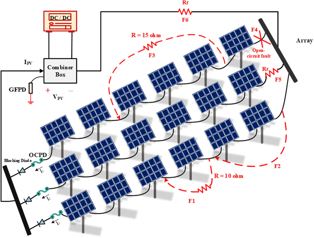
Figure 1. Typical 3 × 6 PV array configuration (3 strings, each includes 6 PV modules).

2.1 Line-to-line (LL) faults

LL faults in PV arrays are defined as a short connection between two different points in a photovoltaic (PV) array with dissimilar potential levels. In-time detection and elimination of LL faults pose a significant challenge for conventional protection devices under specific conditions, such as high fault impedance, faulty module involvement, etc. LL faults can happen because of three main causes (Zhao et al., 2013):

• An accidental short-circuit between two current-carrying conductors (CCCs),

• Serious breakdown in cables insulation,

• Internal shorting in DC junction boxes may happen due to mechanical damage, water ingress, and corrosion.

In the event of LL faults, the voltage of the faulty string can suddenly drop, resulting in an additional reverse current flow from the healthy strings and modules into the fault location. Therefore, a protection device is needed in place to identify the additional current in PV strings. According to the U.S. National Electrical Code (NEC), a single overcurrent protection device (OCPD) is required in series with each string to safeguard PV modules and conductors. The OCPD rated current should not exceed 1.56 of the PV array short-circuit current (I_SC) at standard test conditions (STC: irradiation = 1000 W/m2, temperature = 25 °C, air mass = 1.5). The installed fuse rating of an OCPD can be calculated as 1.35 × 1.56 I_SC = 2.1 I_SC, given that a typical fuse minimum breaking capacity is 1.35 of the circuit-rated current (Pillai et al., 2019).

However, LL faults may not generate sufficient fault currents to trip the OCPDs for various reasons, such as low irradiation levels, high fault impedance, faulty module involvement, and a maximum power point tracker (MPPT). As a result, the faults may go unnoticed in PV arrays for an extended period, leading to significant damage and catastrophic consequences.

Figure 1 provides a depiction of LL faults within PV strings. The concept of mismatch percentage, which is calculated as Equation 1, is used for LL faults severity assessment.

$mismatchpercentage=\frac{numberoffaultymoduleinastring}{numberofallmodulesinastring}\times 100(1)$

The diagram in Figure 1 depicts three types of LL faults: F₁, which has a 16.67% mismatch, F₂, which has a 33.33% mismatch, and F₃, which has a 50% mismatch. The severity of LL faults can also be determined by the accompanying fault impedance values, which may range from zero to several ohms depending on the fault path. In Figure 1, F₁ and F₃ show LL faults with 10 and 15 Ω of fault impedance, respectively, whereas F₂ has a fault impedance value of zero.

This research delves into the impact of short circuit faults on different numbers of modules at five distinct levels. These levels include one, two, three, four, and five modules, and each level exhibits a mismatch percentage at 16.67%, 33.33%, 50%, 66.67%, and 83.33%, respectively. The study examines fault impedance within the range of 0–25 Ω, with a 5 Ω interval between each step. In contrast, the PV array I-V curve under normal and different LL fault scenarios is illustrated in Figure 2A which highlights two important facts about LL faults. Firstly, when LL faults impact the I-V curves under low mismatch levels and high impedances, they behave similarly to normal conditions, making it challenging to identify faulty conditions. Secondly, I-V curves affected by LL faults under high mismatch levels and high impedances behave similarly to LL faults at low mismatch levels and low impedances, presenting another challenge in classifying faulty conditions.

Figure 2

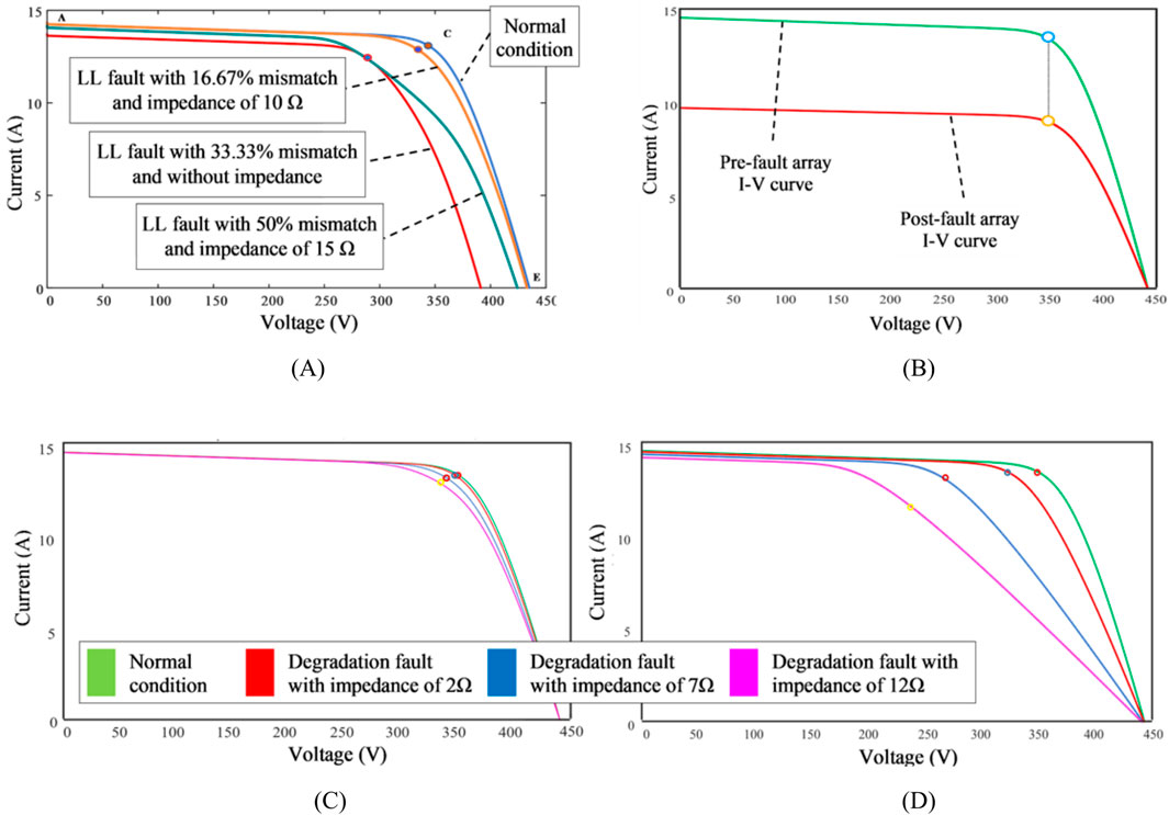
Figure 2. (A) The impact of different mismatch levels and fault impedance on I-V curve during an LL fault (B) The impact of an open-circuit fault on the I-V curve (C) A degradation fault in a string (D) A degradation fault in the whole array.

2.2 Open-circuit (OC) faults

Basically, open-circuit (OC) faults happen when CCCs accidently break. This can occur because of crackings in PV modules (or PV cells), or connections between modules (i.e., wiring and junction boxes). F₄ in Figure 1, shows an OC fault, which might have occurred due to any of the above-mentioned reasons. Assuming that the mentioned OC fault has occurred under STC, it generates only a small amount of fault current (Harrou et al., 2018). As one out of three strings is disconnected, more than a third of the output power is lost. According to Figure 2B, during an OC fault, the PV array operating point voltage remains unchanged. However, the PV array current is mainly affected in an OC fault. Accordingly, if more strings are disconnected, there is less short-circuit current (I_SC). Therefore, when n strings are disconnected as a result of an OC fault, the PV array short circuit current will be mI_SC–nI_SC = (m - n)I_SC, for a PV array with m strings, in which n strings are disconnected (see Figure 2B).

2.3 Degredation faults

PV modules and arrays are a reliable source of energy, but they are susceptible to be degraded, especially after an long time (Santhakumari and Sagar, 2019). Optical degradation caused by prolonged exposure to UV radiation, cell degradation caused by a decrease in shunt resistance (R_sh), a relative increase in series resistance (Rs), or module short circuit current (I_SC), and mismatched cells due to crackings in cells, soiling on cell surface, partial shading and other factors can all cause PV module degradation (Meyer and Van Dyk, 2004). Numerous studies have already investigated degradation faults (Pei et al., 2020), so our research focused only on the impact of series resistance. In this study, both array and string degradation faults are investigated by incorporating Rs once in the output of an array and then throughout a string. As shown in Figure 1, F₅ demonstrates a string degradation, whereas F₆ dipicts an array degradation fault. Also, Figure 2C shows the impact of degradation faults on a PV string I-V curve emulated using various Rs values. Although a relatively high (12 Ω) resistance value is implemented, the string I-V curve under a degradation fault looks the same as that in normal condition. Besides, Figure 2D shows the impacts the PV array I-V curve may experience during an array degradation fault with different Rs values. As the Rs value is increasing, the curve is behaving very differently compared to a normal condition curve.

Regarding the fact that conventional protection devices are unable to detect and clear the faults in PV arrays particularly under critical fault detection conditions, powerful modern and reliable fault detection approaches and strategies which are able to detect the faults early and in time are more noticeably required.

2.4 Review of related work

To overcome the challenges of conventional strategies and provide modern automatic fault detection and classification schemes, artificial intelligence (AI) and more specifically machine learning (ML) have gained in popularity and appeared in literature in recent years (Thakfan and Bin Salamah, 2024). Initial approaches relied on individual machine learning classifiers, with commonly used models including Decision Tree (DT), Support Vector Machine (SVM), Logistic Regression (LogR), Naïve Bayes (NB), and k-Nearest Neighbors (kNN), among others (Gaviria et al., 2022).

In Yahyaoui et al. (2023), a one-class fault detection scheme is presented which is based on comparing various single classifiers and different groups of features. The final model selects k-nearest neighbors (kNN) classifier and a specific group of features as the most accurate combination. A similar approach is also used in Hichri et al. (2024) which support vector machine (SVM) classifier performs the best when features are selected using salp swarm algorithm (SSA). Deep learning algorithms have been adopted in Hajji et al. (2023) which a bidirectional long-short term memory (BiLSTM) classifier shows an accurate performance in fault detection and classification. In, machine learning and ensemble learning methods were evaluated for diagnosing complex PV faults, achieving high detection accuracy. In another study (Amiri and Kichou, 2024), a convolutional neural network (CNN) and bidirectional gated recurrent unit (Bi-GRU) prove to be efficient in detecting and classifying various PV faults. However, all previously mentioned models are able to detect and classify only the faults with high severity. Severe faults are the easiest anomalous conditions to detect, therefore they have neglected the most difficult and critical conditions for fault detection in PV arrays. Note that critical fault detection conditions are when a few modules (usually a single module) is engaged in the fault which is also accompanied by a critical (usually high) impedance value. The condition are named critical since they result in a faulty condition which is very similar to PV array normal (no-fault) condition and makes the process of detection very difficult (or sometimes impossible).

Many studies can be found in literature that have taken into consideration the critical conditions in fault detection. However, some drawbacks can be seen in their proposed models. Reference (Amiri and Oudira, 2024) presented an accurate model to detect and classify several faults in PV arrays even under a few critical fault detection condition. But the main drawback is that the presented model requires a massive dataset to be fully trained, while real-world data samples can sometimes be extremely challenging to collect particularly in harsh weather conditions. Authors in Badr et al. (2021), Dhimish and Tyrrell (2023), Hong and Pula (2024), Suliman et al. (2024) have considered a small dataset in model training process. However, the presented models are not accurate enough to be implemented in real condition.

To increase the final model accuracy, various novel techniques such as stratification is employed. The mentioned technique is used in Kumari and Panigrahi (2024) which attempts to detect various faults in PV arrays. In Kumari and Panigrahi (2024), the whole fault detection process is divided into multiple steps, each of which takes its own related responsibility. However, the most important drawback of the model is that due to the high interdependency between the steps, in case a single misclassification occurs, especially in initial levels, the misclassified sample flows through the whole model and reduces the final model reliability.

To consolidate the recent literature on PV fault detection, Table 1 provides a comparative summary of representative studies. It highlights the datasets, fault types, methods, and key findings, thereby illustrating the progress and limitations of state-of-the-art approaches.

Table 1

Table 1. Review of related works.

In order to fill the gaps and overcome the challenges, a novel model is proposed in this study to detect and classify various kinds of faults in PV arrays. Initially, a group of machine learning (ML) classifiers are arbitrarily selected. Then, fuzzy logic (FL) system nominates the potentially capable classifiers. After that, particle swarm optimization (PSO) algorithm yields the optimal combination of the previously nominated classifiers by FL. Finally, six combination rules are considered to combine the output prediction of each classifier and produce the final output prediction. To provide a more accurate prediction, PSO is again employed to assign and optimize weights to each individual classifier. To train the model, several features are extracted from the PV array I-V curve under normal and fault conditions using Manhattan distance (MD) and Chebyshev distance (CD) methods. The permutation feature selection technique is then utilized to determine the importance of features, and select the best and most effective features to reduce the dimensionality of the dataset and thus the complexity of the training process. After the final model including the selected classifiers by PSO and the nominated combination technique is fully trained and validated using the training dataset containing only the selected features by the permutation feature selection technique, it is then further verified and tested using a test (unseen) dataset.

Therefore, the primary contributions of this study can be described as follows:

• The final model aggregates the most accurate classifiers and eliminates the ones which are not able to perform accurately. This remarkably increases its reliability in the process of fault detection and classification since all the classifiers are systematically selected through the fuzzy logic and PSO based process of classifier selection and optimization. The optimal number of classifiers to form the final model with respect to an increase in simplicity and accuracy is also determined using the PSO technique.

• Multiple combination techniques and rules are utilized to combine the output prediction of each individual classifier and provide the most accurate final result. In order for the final model to produce an even more accurate final prediction, PSO is also employed to assign and optimize a unique weight to each individual classifier.

• Numerous features have been utilized in past models from the PV array I-V curve. However, this study proposes the Manhattan distance and Chebyshev distance techniques to extract various features from the PV array I-V curve according to five predefined points. In addition, to avoid redundancy and select only the most effective features thus reducing the dataset dimensionality and making the final model less computationally complex, the permutation feature selection technique is employed.

• To demonstrate the model high capability of fault classification, the final model is experimented under various faults critical conditions (i.e., critical impedance values and/or low mismatch levels) which are proven to be the most challenging conditions for PV array faults to be detected.

3 The proposed fuzzy logic and PSO based fault detection methods

The present study proposes a novel idea to detect and classify various frequent faults in PV arrays. The presented model combines the predictions from various individual ML classifiers to make accurate decisions in detecting and classifying faults in PV arrays. The chart of the proposed method is shown in detail in Figure 3. As shown, first, the initial dataset is collected according to the PV array I-V curve under a wide range of normal and faulty conditions. Then, the dataset is pre-processed and several features are constructed based on Manhattan distance (MD) and Chebyshev distance (CD) techniques.

Figure 3

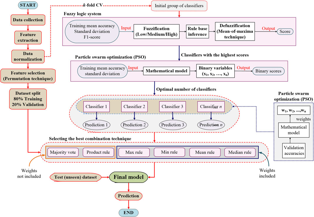
Figure 3. Proposed fuzzy logic and PSO based method for fault detection and classification in PV array.

Next, a group of classifiers are arbitrarily selected and trained using the whole normalized dataset. To initially select the best classifiers, each individual classifier is assigned a score using fuzzy logic (FL) system based on the classifier training mean accuracy, standard deviation, and F1-score and the classifiers with the highest scores are nominated. After that, the particle swarm optimization (PSO) technique determines the optimal number of classifiers through a binary (0 or 1) classification. In the meanwhile, the permutation feature selection technique is applied to the normalized dataset to select only the most effective features and reduce the dataset dimensionality. The dataset is then split into training subsets with 80% and validation subset with 20% of the whole dataset. To combine the prediction of each individual classifier, various combination techniques, such as min rule, max rule, product rule, mean rule, median rule, and majority vote rule are tested and finally the best technique is ascertained. To produce a more accurate final result, PSO technique is again employed to assign and optimize weights for specific combination techniques, namely min rule, max rule, mean rule, and median rule. In the end, the finally created model is further evaluated using an test (unseen) dataset.

3.1 Initial dataset creation

The initial data samples are collected by defining five specific points on the PV array I-V curve under normal and faulty conditions in various environmental settings, including different temperature and irradiance levels. As illustrated in Figure 4A, the pre-defined points are labeled as A-E and are explained below.

• “A” represents a point where I_PV = I_SC and V_PV = 0.

• “B” is a point where V_PV = V_OC/2 with the corresponding current which is known as I (half-V_OC) in this study.

• “C” refers to a point where I_PV = I_MPP and V_PV = V_MPP.

• “D” is a point where I_PV = I_SC/2 with the corresponding voltage which is known as V (half-I_SC) in this study.

• And finally “E” represents a point where V_PV = V_OC with I_PV = 0.

Figure 4

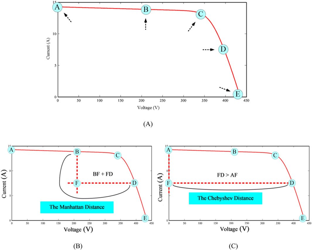
Figure 4. (A) Pre-defined points on a PV array I-V curve to construct the initial dataset (B) Example of Manhattan distance technique in feature extraction process (C) Example of Chebyshev distance technique in feature extraction process.

3.2 Feature extraction process

Feature extraction techniques are usually utilized to provide the ML classifiers with more understandable interpretation of the initial datasets. In this study, two distance-based feature extraction techniques, namely the Manhattan distance (MD), and the Chebyshev distance (CD) are employed. Manhattan and Chebyshev distances are computationally more efficient than Euclidean distances and tend to perform better in high-dimensional spaces. The Manhattan distance is more robust to outliers, while the Chebyshev distance effectively captures the maximum variations across coordinates. The Manhattan distance, sometimes referred to as L1 distance or city block distance, is calculated using Equation 2. It measures the dissimilarity between two data points regarding their positional deviation along a graph X and Y axes (Yang, 2019).

$Manhattandistance=\left|x_2-x_1\right|+\left|y_2-y_1\right|(2)$

where the pairs (x₁, y₁) and (x₂, y₂) represent the respective coordinates of the two points. As shown in Figure 4B, the Manhattan distance between the points B and D can be calculated as BD_Manhattan = BF + FD. Besides, the Chebyshev distance, also known as the L $\infty$ or chessboard distance, quantifies the maximum difference between the corresponding features of two data points using Equation 3. It measures the dissimilarity between two data points on any axis in a graph (Coghetto, 2016).

$Chebyshevdistance=\mathit{max}\left(\left|x_2-x_1\right|,\left|y_2-y_1\right|\right)(3)$

where the pairs (x₁, y₁) and (x₂, y₂) represent the respective coordinates of the two points. As shown in Figure 4C, the Chebyshev distance between the points A and D can be calculated as AD_Chebyshev = max (AF, FD) = FD. Finally, all extracted features are listed in Table 2.

Table 2

Table 2. Extracted features from PV array I-V characteristic curves.

3.3 Data normalization

During data pre-processing, it is essential to normalize data attributes to maintain their intrinsic nature. This process aims to improve feature type consistency and minimize redundancy within the dataset. In this study, Z-score normalization technique is utilized in which features are distributed as X ∼ N (μ = 0, σ2 = 1) centered at a mean of 0 and a variance (σ2), thus standard deviation (σ) of 1. This approach is preferred to ensure that the feature columns follow a standard normal distribution. The mathematical representation of Z-score normalization process can be seen in Equation 4.

$x_{\left(normalized\right)}=\frac{x-\mu \left(X\right)}{\sigma \left(X\right)}(4)$

In Equation 4, X = {x₁, … , x_n} represents the feature vector including n samples, and x denotes a single sample in X.

3.4 Fuzzy logic (FL) system

3.4.1 Fuzzification

The use of fuzzy logic (FL) in decision-making is particularly effective in uncertain and ambiguous situations, as it can produce more accurate results. This is accomplished by assigning degrees of membership between 0 and 1 to elements, indicating their membership in a particular set, through the creation of membership functions (MFs) (Rios et al., 2021). Several kinds of MFs can be used in FL systems, such as triangular, sigmoid, trapezoidal, gaussian, etc. (see Figure 5A).

Figure 5

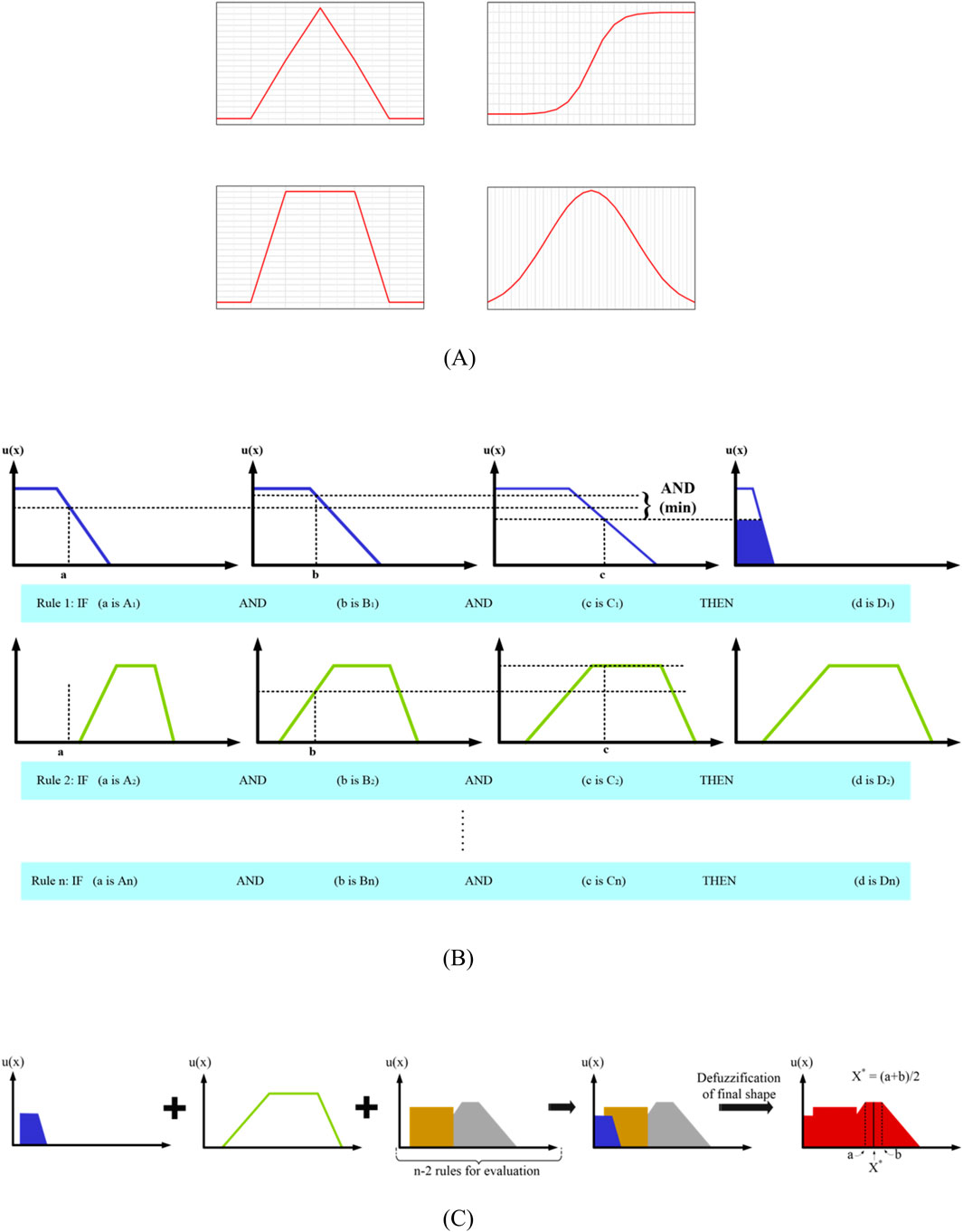
Figure 5. (A) Several fuzzy logic membership functions: triangular, sigmoid, trapezoidal, and gaussian (B) Evaluation of rules in the process of inferencing (C) Aggregation of rules and defuzzification of final shape.

In this study, trapezoidal MFs are utilized to examine four fuzzy variables: training mean accuracy, standard deviation, F1-score, and output as the output result of the aggregation of three other variables. Additionally, the range of values for each variable is established using arrays with a certain step size. The impact of input on output in FL is primarily determined by MFs, with the trapezoidal function being widely used due to its ability to transform complex inputs into a fuzzy form using two slope change points, thus increasing the membership range compared to more straightforward functions. Moreover, the dual points of slope alteration in the trapezoidal membership function allow for precise parameter configurations, enabling the desired input influence on output adjustment. For this problem, the trapezoidal membership function is defined and utilized as Equation 5.

$u\left(x;a,b,c,d\right)=\left\{\begin{array}{ll}0& x\le a\\ \frac{x-a}{b-a}& a\le x\le b\\ \begin{array}{l}1\\ \frac{d-x}{d-c}\\ 0\end{array}& \begin{array}{l}b\le x\le c\\ c\le x\le d\\ x\ge d\end{array}\end{array}\right.(5)$

where u(x) is the normalized data, x is the data extracted from the datasets and a, b, c and d are the values referring to the data on x-axis belonging to highest and lowest pertinence degree.

3.4.2 Inference system

After fuzzification, the values of the pertinence degree generated in each input variable are passed to the set of fuzzy rules which must cover all possible situations of the behavior of the fuzzy system. The number of rules are mathematically calculated as Equation 6.

$N_{rules}=n^m(6)$

where n is the number of categorical values and m shows the number of input variables. In all of the rules, the Mamdani inference model (Mamdani and Assilian, 1999) is applied, in which the logical operator ‘‘AND’’ is used over the antecedents of each rule, being the lowest value chosen as a consequence among the values of the pertinence degree of the triggered rule. To this end, fuzzy numbers are utilized to assess the membership degree of each input variable, and a series of rules are created to combine the mentioned degrees. These rules include a certain number of unique combinations of the three input variables membership degrees, and the activation degree for each rule is determined by taking the minimum membership degree of the input variables. Finally, the activation degree for each possible value of the output is calculated by considering the minimum activation degree for all rules linked to that value. The activation levels obtained are then aggregated across the entire spectrum of output values. A designated function is used to calculate the highest activation level of the non-fuzzified outcome and the degree of membership of the fuzzified output value.

As stated, the firing level for each rule is determined using the min operator shown in Equation 7. If the AND operator appears in the antecedents part, the minimum fuzzified value will be selected (see Figure 5B). As shown in Figure 5B, Rule 2 is not activated because the input value a has zero membership degree for the linguistic value A2, which has the minimum fuzzified value based on the AND operator.

$u_{A\cap B\dots N}\left(x\right)=\mathit{min}\left[u_A\left(x\right),u_B\left(x\right),\dots ,u_N\left(x\right)\right](7)$

where A, B, … , N are fuzzy sets with membership functions uA(x), uB(x), …, uN(x) respectively.

In this study, this methodology employs the training mean accuracy, standard deviation, and F1-score as input variables, along with an output variable that represents the score achieved by each classifier, adhering to predetermined standards to assess efficacy and determine scores.

3.4.3 Defuzzification

At the end, the defuzzification module starts after all the rules were triggered by the inference module. In order to transform the values of the pertinence degree, selected as consequent by the inference module, into an accurate output of numerical values, it is necessary to defuzzify them. For this, the mean of maxima (MoM) method is used, because it is one of the most used in fuzzy expert systems. In this method, the defuzzified value is taken as the element with the highest membership values. When there are more than one element having maximum membership values, the mean value of the maxima is taken. The MoM (X*) is given by Equation 8 (Mondal et al., 2017):

$X^{*}=\left[{\sum }_i{u}_i\left(x\right)\times \mathit{max}\left\{y_i\right\}\right]\times {\left[{\sum }_i{u}_i\left(x\right)\right]}^{-1}(8)$

where ${\mathrm{u}}_{\mathrm{i}}\left(\mathrm{x}\right)$ represents the membership function value of the fuzzy set at point x, y_i represents the value of the universe of discourse corresponding to the membership function ${\mathrm{u}}_{\mathrm{i}}\left(\mathrm{x}\right)$ and max{y_i} represents the maximum value among the values of the universe of discourse that correspond to the maximum membership values of the fuzzy set. In this way, based on the generated results, the system can give a score to each of the classifiers, and the higher score indicates that the classifier is superior to the others. Figure 5C shows the calculated MoM of the final output fuzzy set for the previous example problem.

3.5 Optimal number selection

Using FL, scores are assigned to each individual classifier in the group of classifiers. Low-scoring classifiers are eliminated, and higher-scoring ones are selected to improve the results. However, determining the optimal number of selected classifiers for maximum effectiveness is complex. Mathematical modeling and optimization techniques can address this issue. According to Equation 9, a mathematical model is created based on statistical metrics, including the training mean accuracy and standard deviation acquired from cross-validation (CV) technique. The objective function and constraints are crucial to the model and depend on the desired outcomes of the classification task.

$\begin{array}{ll}\hfill & \hfill objectivefunction=\mathit{max}\left({\sum }_{i=1}\left(x_i\times {trainingmeanaccuracy}_i\right)\right.\\ \hfill & \left.-\beta \left(1500\times {\sum }_{i=1}\left(x_i\times {std}_{i\_\left(normalized\right)}\right)\right)\right)subjectto:{\sum }_{i=1}{x}_i=n\left(x_i\in \left\{0.1\right\}\right)\hfill \end{array}(9)$

Equation 9 is developed to address the challenge of maximizing training mean accuracy while minimizing standard deviation simultaneously. The proposed method involves a composite function that combines the training mean accuracy and the negative standard deviation with a weightage factor β that allows to adjust the balance between precision and variability based on the objectives and preferences. The decision variables in this model are binary variables x_i, where n is the number of classifiers selected from a set of N available classifiers. These variables take the value of 1 if the classifier is selected and 0, otherwise. The model constraints ensure that exactly n classifiers are selected, and each binary variable takes on one of two possible values (i.e., 0 or 1). The ${\text{training}\text{mean}\text{accuracy}}_{\mathrm{i}}$ and ${\text{std}}_{\mathrm{i}\_\left(\text{normalized}\right)}$ of the selected classifiers represent the variables, with efforts to align the standard deviation with the accuracy scale through standardization. In the subsequent analysis, a coefficient of 1500 which is calculated according to the trial-and-error technique is employed to amplify the standard deviation impact on the objective function. Equation 9 is finally addressed using the PSO technique.

3.6 Feature selection process

Feature selection techniques are utilized to select a relevant subset of features from a dataset. They offer two primary benefits, which include enhancing the performance of classification problems and simplifying model interpretation by discarding irrelevant features. In this study, the permutation method is utilized to perform a feature selection to identify the most important features which can affect the accuracy of the final model.

The permutation method which is basically grounded in mathematical permutation (see Equation 10) severs the connection between the input (feature) and the target (class) and haphazardly rearranges the values for a pre-determined number of iterations.

$P\left(\begin{array}{c}n\\ r\end{array}\right)=\frac{n!}{\left(n-r\right)!}\left(r\le n\right)(10)$

In Equation 10, n shows the total number of samples in a feature and r is a subset of n samples. In the process of feature selection in this study, n = r, meaning that all samples (values) of a specific feature take part in permutation process and thus no value is excluded from the feature vector. Therefore, Equation 10 can be simplified as Equation 11.

$P\left(\begin{array}{c}n\\ n\end{array}\right)=n!(11)$

Therefore, according to Equation 11, a feature can present n! different states when all values are considered in the permutation process (Let n! = m). The model is then trained using the dataset which includes one permuted (shuffled) feature and yields a specific score (e.g., accuracy) after each state (see Figure 6). In Figure 6, V_i (i = 1, … , n) are different values of n samples of a specific feature.

Figure 6

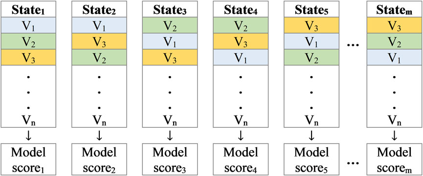
Figure 6. Scores in m different states of permutation.

The final permutation score can be calculated as Equation 12 in which k is a hyperparameter and denotes the number of permutation subsets which are randomly selected (i.e., k subsets of m total possible subsets).

${modelscore}_{permutation}=\frac{1}{k}{\sum }_{i=1}^k{\left(modelscore\right)}_i\left(k\le m\right)(12)$

As shown in Equation 13, the final permutation score shows a deviation with the model actual score (i.e., before permutation). Therefore, the more “model score deviation”, the more importance in the specific feature which shows that the target is more dependent on that specific feature.

$modelscoredeviation={modelscore}_{actual}-{modelscore}_{permutation}(13)$

In practice, permutation importance was implemented using the scikit-learn library. For each feature, the values were randomly shuffled while keeping the other features fixed, the model was re-trained, and the accuracy drop was recorded. This procedure was repeated 20 times for each feature, and the average score was reported as the final importance measure.

Finally, to determine the optimal input (feature) space, a dataset including only the first important feature enters the model and the score of the model is obtained. This proceeds as the next important inputs are added during the next stages and the score of the model is calculated at the end of each stage. Finally, the best input (feature) space is selected based on model scores.

3.7 Weight optimization

To provide more accurate final results, the process of combining the output predictions of multiple classifiers can be accompanied by assigning weights to each individual classifier. However, achieving the optimal set of weights can be a complex optimization problem, mainly when dealing with many classifiers. This is due to the high-dimensional and non-linear nature of the weight space, which may require unconventional optimization methods to reach the global optimum.

Among various optimization algorithms, PSO is selected for its strong global search capability, rapid convergence, and flexibility in tackling complex, high-dimensional optimization problems. Unlike gradient-based methods, PSO uses a population-based stochastic approach that allows it to explore the solution space effectively, making it ideal for non-differentiable and multimodal functions. Its computational efficiency and ability to balance exploration and exploitation contribute to its competitive performance, even in the face of advanced optimization techniques. In PSO, a swarm of particles navigates through the search space, working together to identify the optimal solution by updating their positions and velocities based on their previous and the swarm global best performance. Equations 14, 15 express the current position and velocity of particle i in the context of PSO.

$x_i=x_{i1},x_{i2},\dots ,x_{iD}(14)$

$v_i=v_{i1},v_{i2},\dots ,v_{iD}(15)$

where D is the dimension of the principal search space.

The determination of the particle i velocity and position is achieved through Equations 16, 17 for calculation purposes.

$v_{id}^{t+1}=\left[w\times v_{id}^t\right]+\left[c_1\times r_{1i}\times \left(p_{id}-x_{id}^t\right)\right]+\left[c_2\times r_{2i}\times \left(p_{gd}-x_{id}^t\right)\right](16)$

$x_{id}^{t+1}=x_{id}^t+v_{id}^{t+1}(17)$

Which involves the use of various parameters such as inertia weight (w), acceleration constants (c₁ and c₂), and random values (r_1i and r_2i) uniformly distributed in [0, 1]. The variables denoted by t and d represent the tth iteration and the dth dimension, respectively. Additionally, the elements of p-best and g-best in the dth dimension are represented by p_id and p_gd. Each particle position and velocity values are updated continuously to locate the optimal set until a stopping criterion is met, which may include a maximum number of iterations or a satisfactory fitness value.

In this study, the particles in the swarm correspond to possible weight assignments, and their movements reflect the search for an optimal set of weights. By using PSO to optimize the weights, the high-dimensional space of possible weight assignments can be efficiently explored and quickly converged to an optimal set of weights that minimizes the overall error rate. Equation 18 has been formulated to fulfill the aforementioned requirements.

$objectivefunction=\mathit{max}\left({\displaystyle \sum _{i=1}^n}{validationaccuracy}_i\times {weight}_i\right)Subjectto:{\displaystyle \sum _{i=1}^n}{weight}_i=1(18)$

In Equation 18, the weight variable of interest is multiplied by the validation accuracy of each classifier, leading them to attain their respective maximum values. This approach aims to optimize the algorithmic performance and achieve the desired outcomes.

3.8 Combination techniques

To obtain a single final prediction, the output predictions produced by classifiers must be combined. In order to combine the output predictions of each classifier, various probability-based techniques exist in literature and can be utilized. The combination task involves assigning sample z to one of m possible classes (C1, C2, …, Cm). Assuming n classifiers are available, each representing z by a distinct predicted class. The predicted class by the ith classifier is denoted by xi. Each class Ck is modeled by the probability density function (PDF) P (xi|Ck), with P(Ck) indicating the prior probability of its occurrence. Based on Bayesian theory, given all the predicted classes xi, z should be allocated to Cj if and only if the posterior probability, P(Ck|xi) is maximum. Equation 19, which refers to Bayesian decision-making theory, shows that in order to achieve an accurate decision based on all available information, it is imperative to meticulously compute the probabilities of various classes by simultaneously considering all predicted classes.

$assignz\to C_{j}ifP\left(C_j|x_i\right)=\underset{k}{\mathit{max}}P\left(C_k|x_i\right)(19)$

Based on Equation 19, six popular existing combination techniques can be briefly summarized as follows, and the formulation is provided in Equations 20–25.

1. The product rule:

$P^{-\left(n-1\right)}\left(C_j\right){\displaystyle \prod _{i=1}^n}P\left(C_j|x_i\right)=\underset{1\le k\le m}{\mathit{max}}{P}^{-\left(n-1\right)}\left(C_k\right){\displaystyle \prod _{i=1}^n}P\left(C_k|x_i\right)(20)$

2. The max rule:

$\underset{1\le i\le n}{\mathit{max}}P\left(C_j|x_i\right)=\underset{1\le k\le m}{\mathit{max}}\underset{1\le i\le n}{\mathit{max}}P\left(C_k|x_i\right)(21)$

3. The min rule:

$\underset{1\le i\le n}{\mathit{min}}P\left(C_j|x_i\right)=\underset{1\le k\le m}{\mathit{max}}\underset{1\le i\le n}{\mathit{min}}P\left(C_k|x_i\right)(22)$

4. The mean rule:

$\underset{1\le i\le n}{\mathit{mean}}P\left(C_j|x_i\right)=\underset{1\le k\le m}{\mathit{max}}\underset{1\le i\le n}{\mathit{mean}}P\left(C_k|x_i\right)(23)$

5. The median rule:

$\underset{1\le i\le n}{\mathit{median}}P\left(C_j|x_i\right)=\underset{1\le k\le m}{\mathit{max}}\underset{1\le i\le n}{\mathit{median}}P\left(C_k|x_i\right)(24)$

6. The majority vote rule:

${\displaystyle \sum _{i=1}^n}{\Delta }_{\text{ji}}=\underset{1\le k\le m}{\mathit{max}}{\displaystyle \sum _{i=1}^n}{\Delta }_{\text{ki}}(25)$

where Δ_ji denotes the ith classifier choice for class j.

3.9 Evaluation metrics

The performance of the proposed model is evaluated using various popular evaluation metrics. Firstly, to ensure a reliable model and avoid overfitting during the training process, the k-fold cross-validation (CV) method is employed to measure the mean accuracy of each individual classifier. Secondly, the confusion matrix, shown in Table 3 is utilized and a comprehensive report of the final model performance is provided through the “accuracy”, “precision”, “recall”, and “F1-score” metrics which are calculated according to Equations 26–29.

$\mathit{Accuracy}=\frac{\mathit{TP}+\mathit{TN}}{\mathit{TP}+\mathit{TN}+\mathit{FN}+\mathit{FP}}(26)$

$\mathit{Precision}=\frac{\mathit{TP}}{\mathit{TP}+\mathit{FP}}(27)$

$\mathit{Recall}=\frac{\mathit{TP}}{\mathit{TP}+\mathit{FN}}(28)$

$\mathit{F}1-\mathit{score}=\frac{2\times \left(\mathit{Precision}\times \mathit{Recall}\right)}{\mathit{Precision}+\mathit{Recall}}(29)$

Table 3

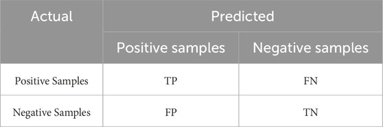
Table 3. Typical 2 × 2 confusion matrix.

The initiations used in Equations 26–29 can be explained as follows:

• TP: The number of positive samples correctly classified by the model.

• FP: The number of negative samples incorrectly classified as positive by the model.

• FN: The number of positive samples incorrectly classified as negative by the model.

• TN: The number of negative samples correctly classified by the model.

4 Model implemention, results, and discussion

4.1 PV array setup

To evaluate the proposed model, a stand-alone experimental PV system including a 3 × 6 PV array (three parallel strings each containing six Yingli YL010D-18 b PV modules in series) has been designed along with a DC-DC boost converter which are depicted in Figure 7. The PV modules used in the setup are rated at 10 W with Voc = 22.5 V, Isc = 0.61 A, V_MPP = 18 V, and I_MPP = 0.56 A. The detailed specifications of the PV modules and the DC-DC boost converter are summarized in Table 4.

Figure 7

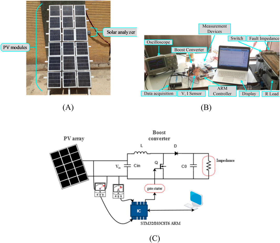
Figure 7. (A) Experimental 3 × 6 PV array (B) DC-DC boost converter and other equipment (C) Data collection station to elicit the PV array I-V curves.

Table 4

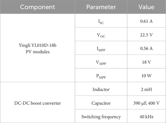
Table 4. PV system specifications.

4.2 Data acquisition process

The initial data samples in this study are acquired using five predefined points on the PV array I-V curves under various environmental (irradiance and temperature) and anomalous (normal or faulty) conditions. To elicit the PV array I-V curves, an I-V curve tracer is developed according to Figure 7C which includes current and voltage sensors, a DC/DC converter, an ARM microcontroller for controlling the switch, and a gate driver circuit. Figure 7C depicts that the duty cycle is regulated by the ARM microcontroller to extract the features from the I-V curve. The STM32f103C8T6 ARM is also used for I-V curve testing algorithm. When testing, voltage and current values are read by the controller. The magnitude of the controller signal is 3.3 V, but the switch requires a minimum of 15 V to remain on. Hence, a gate driver is used to supply the MOSFET necessary voltage. Two voltage regulators power the controller and output circuits of the driver. One produces 3.3 V for the ARM microcontroller, while at the same time, the other generates a 15 V controllable voltage for the gate driver. This tracking algorithm is straightforward in which the PV array initially supplies a low-resistive load to produce a high current level, with a low-duty cycle (approximately 10%). In this case, the PV array yields a low amount of current which is almost equal to the PV array short circuit current. This process is repeated with incremental rises in the duty cycle until it reaches a specific range (over 80%). Finally, the OC voltage is determined by measuring the PV array output voltage in an open circuit state.

During the experimental data collection process, 2936 samples are collected under different conditions, such as no-fault conditions, open circuit faults, line-to-line faults, and degradation faults. The initial dataset includes 2600 training samples and 336 samples for testing the final model which is further detailed in Table 5.

Table 5

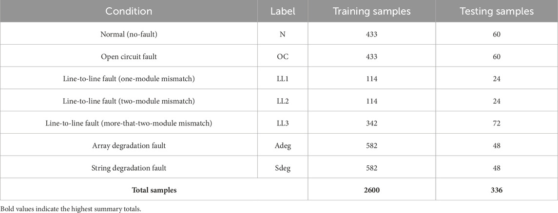
Table 5. Detailed number of data samples.

Once the initial dataset is collected, various features are extracted according to Table 2 and the data samples are normalized using Z-score normalization technique based on Equation 4.

4.3 Experimental results

During the initial stage, each classifier is assessed individually, using the training mean accuracies, standard deviations, and F1-scores as determinants for selecting the initial classifiers by entering the FL process. Figure 8 shows the training mean accuracies and F1-scores as well as standard deviations (highlighted in boxes) produced by ten machine learning classifiers when they are trained using the whole normalized dataset.

Figure 8

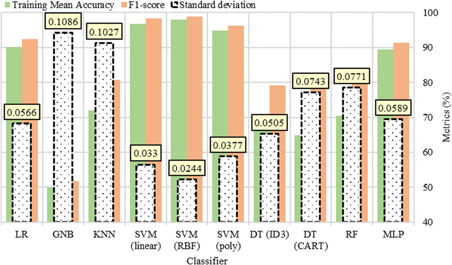
Figure 8. The evaluation metrics and standard deviation of each individual classifier.

4.3.1 Fuzzification

After completing the initial step, the fuzzy system is set up with three linguistic terms; “low,” “medium,” and “high”, for each input variable: training mean accuracy, standard deviation, and F1-score. It is certainly worth mentioning that the linguistic terms are set based on the variable acceptability in the final model creation. Therefore, for instance, a “low” in training mean accuracy and F1-score denotes a low real value in these variables which is not acceptable. However, a “low” in standard deviation shows a high real value in this variable which is also unacceptable. 1n addition, a variable named “output” is also defined as the output result to determine whether the aggregation of three other variables will be either “low”, “medium”, or “high”. In this study, trapezoidal membership function is selected to standardize the data values for all components (see Figure 9A). The range of values for each variable is determined based on the values of evaluated variables (training mean accuracy, standard deviation, F1-score, and output).

Figure 9

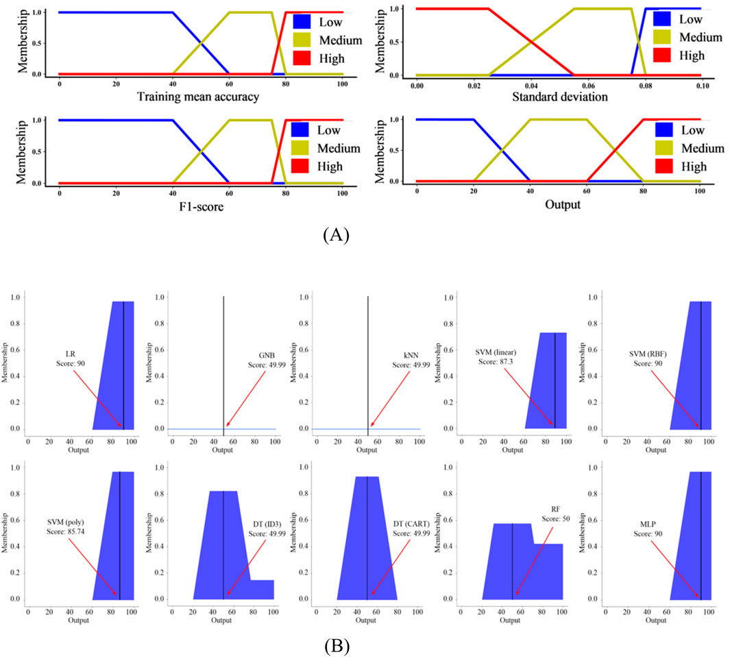
Figure 9. (A) Membership functions for training mean accuracy, standard deviation, F1-score and the output (B) MoM-based defuzzification of final shape in each classifier.

4.3.2 Inferencing

After the fuzzification process, the corresponding degree values generated in each input variable are transferred to a set of fuzzy rules. The number of rules designed to cover all potential situations of fuzzy system behavior according to Equation 6 with n = 3 categorical values and m = 3 input variables will be 3³ = 27 as shown in Table 6.

Table 6

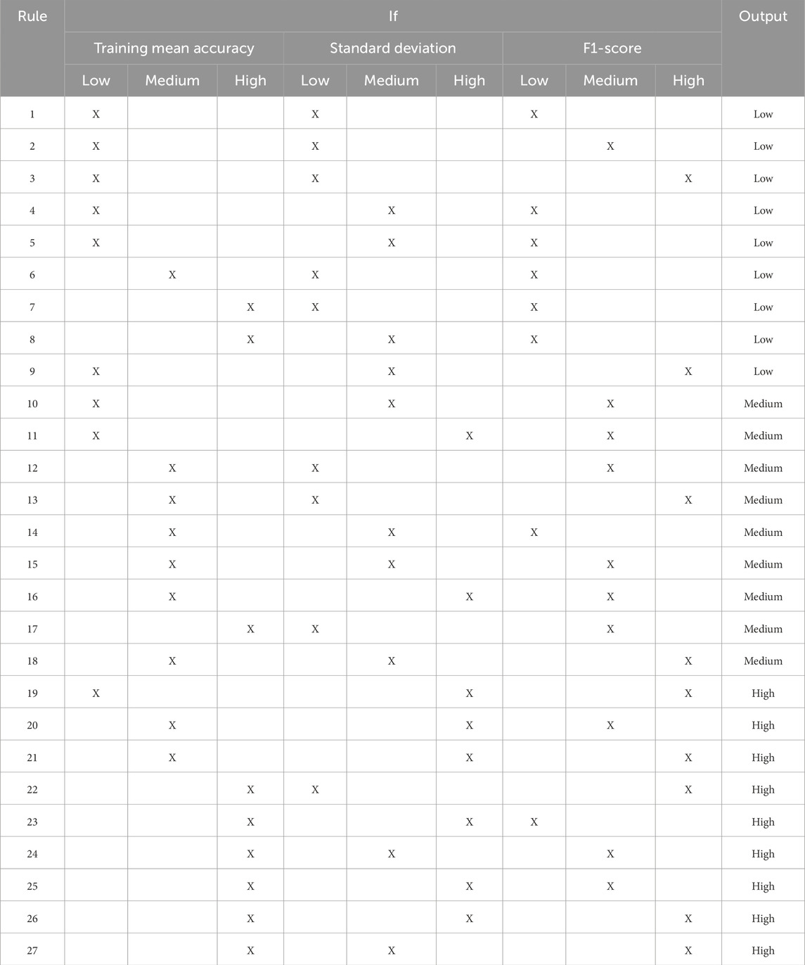
Table 6. Set of base rules of the inference module.

4.3.3 Defuzzification

Following the application of fuzzy logic and subsequent fuzzification, each individual classifier is assigned a score between 0 and 100 according to MoM defuzzification technique and based on three metrics: training mean accuracy, standard deviation, and F1-score (see Figure 9B). The resulting scores serve as an index of classifiers well-suited for the combination. Figure 9B displays the classifiers scores based on MoM defuzzification technique. In this study, the classifiers with the score of 50 and above are selected for the combination which, according to Figure 9B, include LR, SVM (linear), SVM (RBF), SVM (poly), RF, and MLP.

In the initial stage of the method, ten classifiers were considered, out of which LR, SVM (linear), SVM (RBF), SVM (poly), RF, and MLP classifiers progressed to the second stage. These classifiers achieved the highest scores in the fuzzy logic filtering process based on Equation 5 which forms part of the mathematical model that optimizes the best combination of classifiers for the final model. After applying the mathematical programming model to the binary feature problem, discrete states (0 or 1) are observed in X = [x₁, x₂, x₃, x₄, x₅, x₆], in which x₁ = LR, x₂ = SVM(linear), x₃ = SVM(RBF), x₄ = SVM(poly), x₅ = RF, and x₆ = MLP (see Figure 10A). The PSO algorithm is then applied to the mathematical programming model, and the optimal state which yields the maximum value of the objective function as [0 1 1 1 0 0], assigning 1 to x₂ = SVM(linear), x₃ = SVM(RBF), and x₄ = SVM(poly) thus selecting them as the optimal classifiers to create the final model. The parameters for PSO algorithm used to select the optimal classifiers are listed and explained in Table 7 (Step 1).

Figure 10

Figure 10. Results of PSO algorithm in obtaining the best combination of classifiers in fault detection (A) Particle Swarm Optimization Results (B) Determining parameter beta (β) with respect to global best fitness.

Table 7

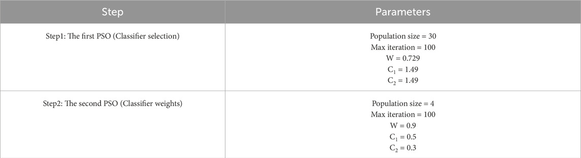
Table 7. Parameters and values used in PSO algorithm in optimization.

It is worth mentioning that based on the parameters outlined in Equation 9; Figure 10B demonstrates that the optimal value for β is 0.5. This outcome is a product of a seamless balance between training mean accuracy and standard deviation, essential for achieving the objective function optimal state (see Equation 9).

Three SVM classifiers with linear, RBF, and polynomial kernels have been selected as the best classifiers to participate in the final model. Before combining the output of each classifier to make the final model, the weight of each classifier needs to be assigned and optimized. This approach prioritizes the classifiers which show higher accuracies as they have substantially more impact on the final model accuracy. A mathematical programming model has been developed for this purpose, and PSO has solved the problem of assigning weights to each SVM classifier with linear, RBF, and polynomial kernels. The PSO variables are explained in Table 7 (Step 2). It's important to note that Step 1 requires further exploration, which is why it employs a larger population, balanced coefficients C₁ and C₂, and a lower inertia weight. In contrast, Step 2 focuses on stability, utilizing a smaller population, reduced coefficients C₁ and C₂, and a higher inertia weight. The most optimal weight values for SVM (linear), SVM (RBF), and SVM (poly) are 0.35, 0.5, and 0.15, respectively. After training these classifiers, it is necessary to perform their validation process during each of the techniques (product rule, max rule, min rule, mean rule, median rule, and majority vote rule) of the combination. These weights are allocated to max, min, mean, and median rule techniques.

The permutation feature selection method has been used to determine the importance of each feature of 20 extracted feature and provides an efficient feature selection process (see Figure 11). According to Figure 11, the permutation technique yields different importance values for the mean rule combination technique in comparison to five other techniques.

Figure 11

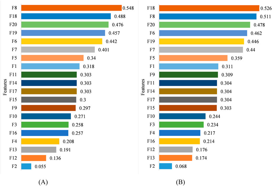
Figure 11. The importance of features in permutation method: (A) scoring features based on their importance in mean rule technique, and (B) scoring features based on their importance in majority vote rule, product rule, max rule, min rule, and median rule techniques.

Finally, the performance of the model is investigated using each combination technique and the selecting the extracted features according to their importance value. Figure 12 demonstrates the training and validation accuracies produced by the model using each combination techniques using a certain number of features, from the most to the least important based on Figure 11. As shown in Figure 12, the mean rule combination technique has been able to produce the highest accuracy during the training process (99.51%) using 11 features which are f₈, f₁₈, f₂₀, f₁₉, f₆, f₇, f₅, f₁, f₁₁, f₁₄, f₁₇, in correct order of importance. Using the corresponding number of features, the mean rule combination technique has also proves to outperform five other combination techniques with 99.81% of accuracy when the model is validated. In addition, Table 8 provides a summarized report of training and validation accuracies as well as the selected features in correct ranking based on Figures 11, 12.

Figure 12

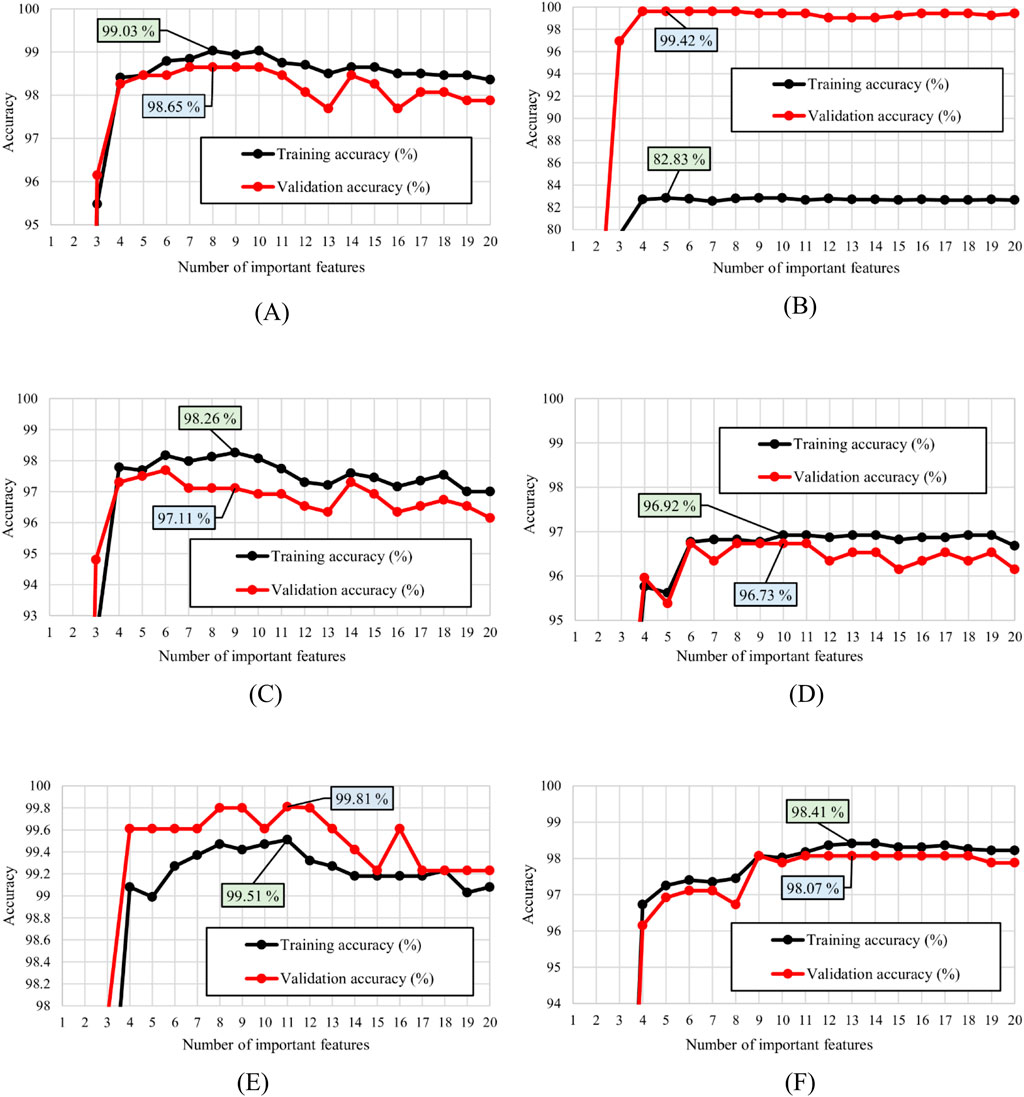
Figure 12. Training and validation accuracies during the permutation feature selection process based on six different rules (A) Product rule (B) Max rule (C) Min rule (D) Median rule (E) Mean rule (F) Majority voting rule.

Table 8

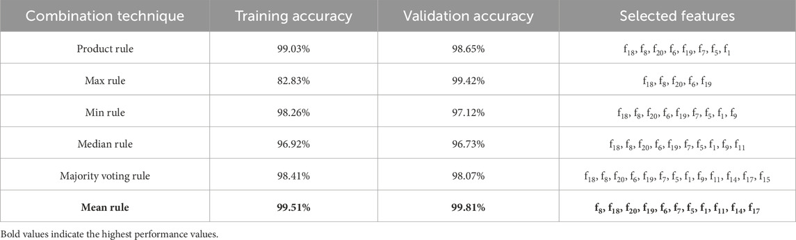
Table 8. Results of model development in training and validation processes.

Furthermore, Figure 13 presents the validation confusion matrices, providing a comprehensive summary of the validation results. It clearly shows the final model accuracy during the validation process by carefully detailing the number of correct and incorrect classifications using different combination techniques. Also, Figure 14 provides information on three other evaluation metrics which are precision, recall, and f1-score which can be extracted from each confusion matrix based on Equations 26–29.

Figure 13

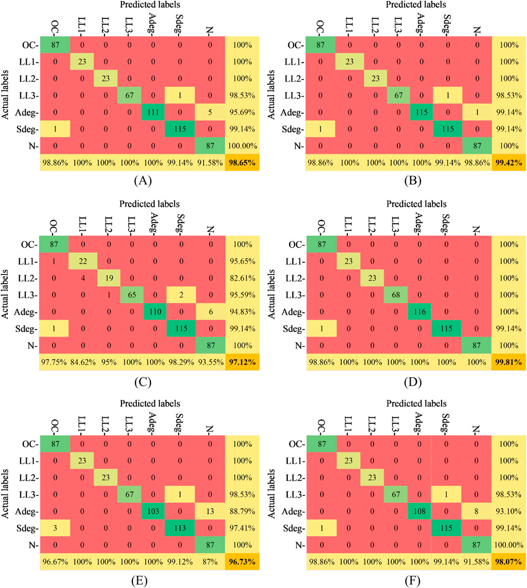
Figure 13. Validation accuracies in different combination techniques (A) Product rule (B) Max rule (C) Min rule (D) Mean rule (E) Median rule (F) Majority voting rule.

Figure 14

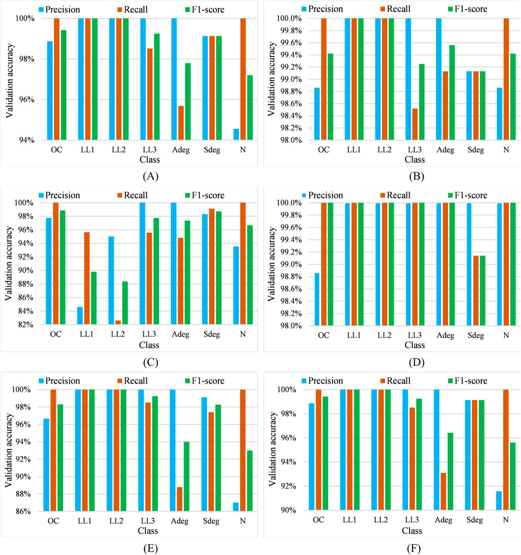
Figure 14. Class-wise validation metric values in different combination techniques (A) Product rule (B) Max rule (C) Min rule (D) Mean rule (E) Median rule (F) Majority voting rule.

Once the final model (including the mean rule combination technique) is selected, the final stage involves using test (unseen) experimental data samples to further verify the model performance. As demonstrated in Figure 15 which include the detailed confusion matrices of using each combination technique, the final model (including the mean rule combination technique) shows the best performance with 97.02% of accuracy during the testing process.

Figure 15

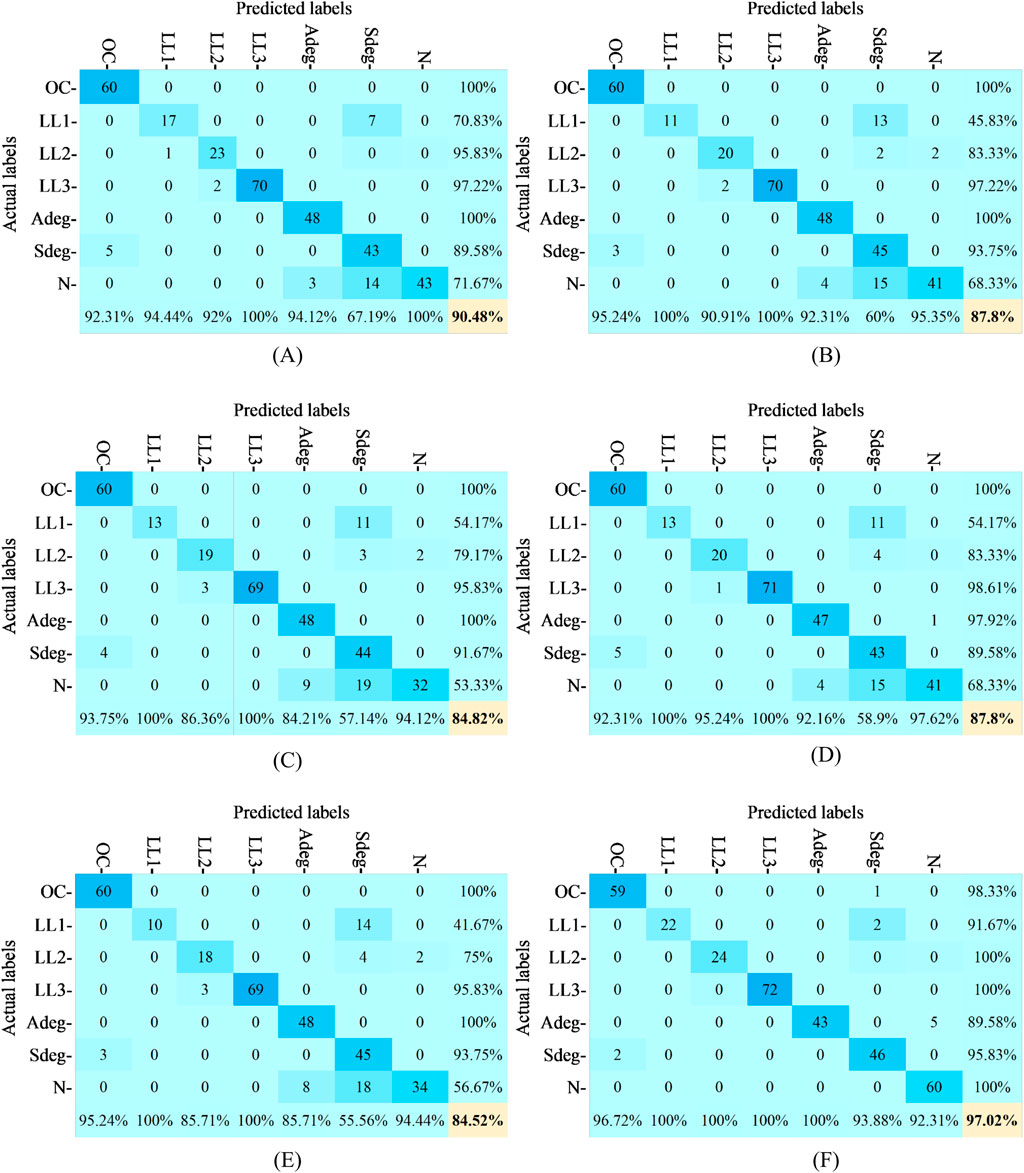
Figure 15. Test accuracies in different combination techniques (A) Majority voting rule (B) Product rule (C) Max rule (D) Min rule (E) Median rule (F) Mean rule.

To provide a more detailed assessment, per-class test metrics (precision, recall, and F1-score) have been reported, as summarized in Table 9. Furthermore, ablation studies have been conducted considering (i) single model vs. ensemble settings, (ii) weighted vs. unweighted fusion strategies, and (iii) the use of top-k features and feature types. The corresponding results are presented in Table 10. These findings clearly indicate the benefits of ensemble learning and weighted fusion, as well as the impact of feature selection on classification performance.

Table 9

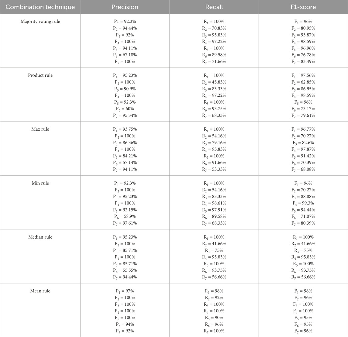
Table 9. Results of model development in testing process.

Table 10

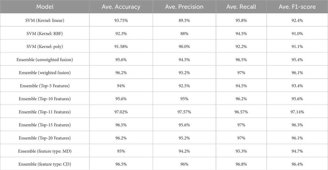
Table 10. Comparison results of ablations in testing process.

4.4 Comparison and a detailed discussion

In order to confirm the superiority of the proposed fuzzy logic and PSO based model, according to Table 11, it is compared to several recent studies in the area of PV fault detection. To provide a fair comparison, various factors are considered, such as the recency of the studies (2023 and 2024), inclusion of modern strategies (e.g., deep learning), various comparison aspects (the ability of severity assessment, the number of required data samples, the consideration of critical conditions for fault detection, and the final experimental accuracies). According to Table 11, the following discussion can be presented:

a. Multiple models in literature, such as Hajji et al., (2023), Yahyaoui et al., (2023), Amiri and Kichou, (2024) have attempted to provide a high accuracy in detection and classification of faults in PV arrays. But, the major disadvantage of all the above-mentioned studies is that none of them have taken into account the critical fault detection conditions. Disregarding the critical fault detection conditions, the process of fault detection becomes absolutely easy to proceed. In addition, the above-mentioned models are not capable of assessing the faults severity to provide a precise instruction for protection devices. To wrap up, despite the fact that these models might apparently look accurate, they are not reliable to be implemented in real world.

b. Authors in Dhimish and Tyrrell (2023), Amiri and Kichou (2024) have positively considered a difficult fault detection condition (critical mismatch levels). Also, the above-mentioned models are capable of assessing the severity of faults in PV arrays. However, it seems that since a challenging fault detection condition is considered, as a result, the model in Dhimish and Tyrrell (2023) is not able to yield high accuracy therefore it looks unreliable in practice. Moreover, model in Amiri and Kichou (2024) requires a massive training dataset to produce a high accuracy.

c. Several disadvantages can also be witnessed in studied such as Hajji et al. (2023), Yahyaoui et al. (2023). Although the previously mentioned models are producing an apparently acceptable accuracy, they need a large number of data samples, have not considered the critical conditions in fault detection, and are not able assess the severity of faults.

d. The model presented in Kumari and Panigrahi (2024) has addressed fault impedance, as another important factor of fault detection conditions (added to critical mismatch levels) that affects the severity of faults in PV arrays. They have also taken considered the severity assessment, and a small dataset for model training process. However, the main drawback is its low accuracy, especially when trying to classify less severe faults.

e. Finally, the proposed fuzzy logic and PSO based model in this study has attempted to overcome all the above mentioned challenges. Initially, unlike previous studies in which the ML classifier selection process was mostly carried out based on a deterministic approach, the proposed model has carefully investigated a vast group of ML classifiers and successfully selected the optimal classifiers which increase its reliability in fault detection and classification process. In addition, optimizing the number of classifiers (PSO), selecting the best combination technique (trial-and-error), and assigning the optimal weights to finally nominated classifiers (PSO) have further improved the final model accuracy and reliability. Moreover, according to Table 11, it can be clearly witnessed that the proposed model in this study outperforms the other recent models in literature since:

• It has considered the most difficult conditions in the process of fault detection and classification (both critical mismatch levels and critical impedance values at the same time).

• It warrants only a small dataset to be fully trained.

• It produces a high accuracy of experimental testing

Table 11

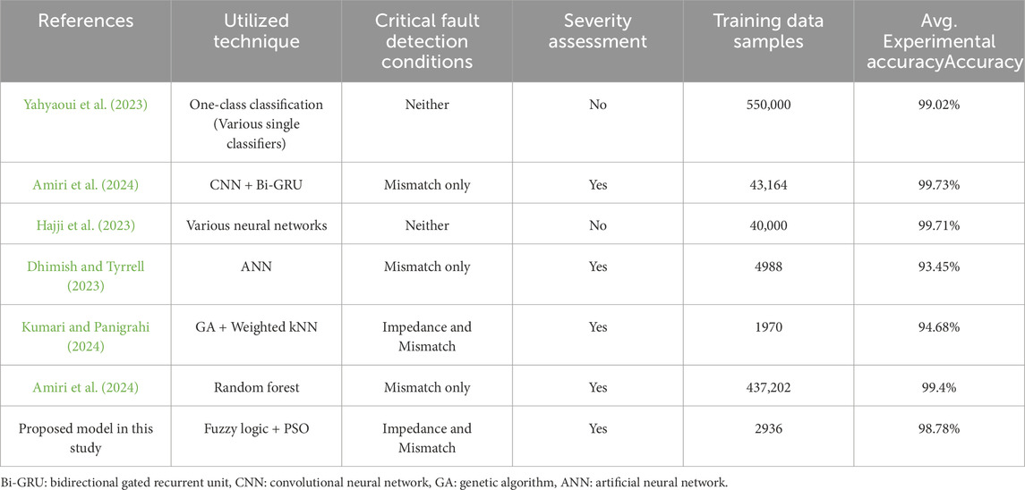
Table 11. FL-PSO model comparison with several recent models in literature.

5 Conclusion

This paper presented a cutting-edge method to detect and classify LL, OC, and degradation faults in PV arrays through I-V curve measurements. Firstly, initial data samples were collected according to five specific points on the PV array I-V curve under various irradiance and temperature conditions. Then, twenty features were extracted from the initial dataset by utilizing the Manhattan distance (MD) and Chebyshev distance (CD) techniques. The model employed various individual machine learning classifiers, such as logistic regression (LR), Gaussian naïve Bayes (GNB), k-nearest neighbors (kNN), support vector machine (SVM), decision tree (DT), random forest (RF), and multi-layer perceptron (MLP). A subset of classifiers with better performance than others were first nominated by fuzzy logic system. Here, fuzzy logic nominated six classifiers LR, RF, MLP, and SVM with three different kernels; linear, RBF, and polynomial kernels. Particle swarm optimization (PSO) technique were then utilized to determine the optimal number of previously nominated classifiers. The optimal number of classifiers optimized by PSO was three including SVM with three different kernels; linear, RBF, and polynomial kernels. To combine the output prediction of each selected classifier, various combination rules were tested, such as min rule, max rule, mean rule, product rule, majority voting rule, and median rule. PSO technique is once again employed to assign optimal weights to each selected classifier. In addition, to reduce the dimensionality of the dataset and simplifying the training process, permutation feature selection technique is used to select the best feature space by determining the importance of each feature. The results showed that the mean rule technique was selected to conclude the final model using 11 selected features according to permutation feature selection technique. The final model showed an outstanding performance among all the other techniques with 98.78% average accuracy.

Data availability statement

The datasets presented in this article are not readily available because The dataset is still confidential. Requests to access the datasets should be directed to bW9oYW1tYWRyZXphLmFnaGFlaUBudG51Lm5v.

Author contributions

PG: Conceptualization, Data curation, Formal Analysis, Investigation, Methodology, Software, Visualization, Writing – original draft. AE: Conceptualization, Data curation, Formal Analysis, Investigation, Methodology, Project administration, Resources, Supervision, Validation, Writing – review and editing. AN: Conceptualization, Data curation, Investigation, Methodology, Software, Visualization, Writing – review and editing. FH: Funding acquisition, Project administration, Resources, Writing – review and editing. PP: Funding acquisition, Project administration, Resources, Writing – review and editing. MA: Investigation, Resources, Writing – review and editing, Conceptualization, Data curation, Formal Analysis, Funding acquisition, Methodology, Project administration, Supervision, Validation.

Funding

The author(s) declare that no financial support was received for the research and/or publication of this article.

Conflict of interest

The authors declare that the research was conducted in the absence of any commercial or financial relationships that could be construed as a potential conflict of interest.

The author(s) declared that they were an editorial board member of Frontiers, at the time of submission. This had no impact on the peer review process and the final decision.

Generative AI statement

The author(s) declare that no Generative AI was used in the creation of this manuscript.

Any alternative text (alt text) provided alongside figures in this article has been generated by Frontiers with the support of artificial intelligence and reasonable efforts have been made to ensure accuracy, including review by the authors wherever possible. If you identify any issues, please contact us.

Publisher’s note

All claims expressed in this article are solely those of the authors and do not necessarily represent those of their affiliated organizations, or those of the publisher, the editors and the reviewers. Any product that may be evaluated in this article, or claim that may be made by its manufacturer, is not guaranteed or endorsed by the publisher.

References

Aghaei, M. (2022). “Introductory chapter: solar photovoltaic energy,” in Solar radiation - measurement, modeling and forecasting techniques for photovoltaic solar energy applications (IntechOpen). doi:10.5772/intechopen.106259

CrossRef Full Text | Google Scholar

Amiri, A. F., Kichou, S., Oudira, H., Chouder, A., and Silvestre, S. (2024). Fault detection and diagnosis of a photovoltaic system based on deep learning using the combination of a convolutional Neural network (CNN) and bidirectional gated recurrent unit (Bi-GRU). Sustain. Switz. 16, 1012. doi:10.3390/su16031012

CrossRef Full Text | Google Scholar

Amiri, A. F., Oudira, H., Chouder, A., and Kichou, S. (2024). Faults detection and diagnosis of PV systems based on machine learning approach using random forest classifier. Energy Convers. Manag. 301, 118076. doi:10.1016/j.enconman.2024.118076

CrossRef Full Text | Google Scholar

Badr, M. M., Hamad, M. S., Abdel-Khalik, A. S., Hamdy, R. A., Ahmed, S., and Hamdan, E. (2021). Fault identification of photovoltaic array based on machine learning classifiers. IEEE Access 9, 159113–159132. doi:10.1109/ACCESS.2021.3130889

CrossRef Full Text | Google Scholar

Coghetto, R. (2016). Chebyshev distance. Formaliz. Math. 24, 121–141. doi:10.1515/forma-2016-0010

CrossRef Full Text | Google Scholar

Dhimish, M., and Tyrrell, A. M. (2023). Photovoltaic bypass diode fault detection using artificial neural networks. IEEE Trans. Instrum. Meas. 72, 1–10. doi:10.1109/TIM.2023.3244230

PubMed Abstract | CrossRef Full Text | Google Scholar

Gaviria, J. F. (2022). “Machine learning in photovoltaic systems: a review,” in Renewable energy. Elsevier Ltd, 298–318. doi:10.1016/j.renene.2022.06.105

CrossRef Full Text | Google Scholar

Ghaedi, P., Eskandari, A., Nedaei, A., Habibi, M., Parvin, P., and Aghaei, M. (2024). Ensemble LVQ model for photovoltaic line-to-line fault diagnosis using K-Means clustering and AdaGrad. Energies 17, 5269. doi:10.3390/en17215269

CrossRef Full Text | Google Scholar

Hajji, M., Yahyaoui, Z., Mansouri, M., Nounou, H., and Nounou, M. (2023). Fault detection and diagnosis in grid-connected PV systems under irradiance variations. Energy Rep. 9, 4005–4017. doi:10.1016/j.egyr.2023.03.033

CrossRef Full Text | Google Scholar

Harrou, F., Sun, Y., Taghezouit, B., Saidi, A., and Hamlati, M. E. (2018). Reliable fault detection and diagnosis of photovoltaic systems based on statistical monitoring approaches. Renew. Energy 116, 22–37. doi:10.1016/j.renene.2017.09.048

CrossRef Full Text | Google Scholar

Hichri, A., Hajji, M., Mansouri, M., Nounou, H., and Bouzrara, K. (2024). Supervised machine learning-based salp swarm algorithm for fault diagnosis of photovoltaic systems. J. Eng. Appl. Sci. 71, 12. doi:10.1186/s44147-023-00344-z

CrossRef Full Text | Google Scholar

Hong, Y. Y., and Pula, R. A. (2024). Diagnosis of photovoltaic faults using digital twin and PSO-Optimized shifted window transformer. Appl. Soft Comput. 150, 111092. doi:10.1016/j.asoc.2023.111092

CrossRef Full Text | Google Scholar

Kumari, P., and Panigrahi, B. K. (2024). Heuristically optimized features based machine learning technique for identification and classification of faults in PV array. IEEE Trans. Industrial Inf. 20, 6089–6098. doi:10.1109/TII.2023.3343729

CrossRef Full Text | Google Scholar

Mamdani, E. H., and Assilian, S. (1999). An experiment in linguistic synthesis with a fuzzy logic controller. Int. J. Hum. Comput. Stud. 51, 135–147. doi:10.1006/ijhc.1973.0303

CrossRef Full Text | Google Scholar

Mellit, A., Tina, G. M., and Kalogirou, S. A. (2018). Fault detection and diagnosis methods for photovoltaic systems: a review. Renew. Sustain. Energy Rev. 91, 1–17. doi:10.1016/j.rser.2018.03.062

CrossRef Full Text | Google Scholar

Meyer, E. L., and Van Dyk, E. E. (2004). Assessing the reliability and degradation of photovoltaic module performance parameters. IEEE Trans. Reliab. 53, 83–92. doi:10.1109/TR.2004.824831

CrossRef Full Text | Google Scholar

Mondal, H. S. (2017). “Enhancing secure cloud computing environment by detecting DDoS attack using fuzzy logic,” in 3rd international conference on electrical information and communication technology, EICT 2017 (IEEE), 1–4. doi:10.1109/EICT.2017.8275211

CrossRef Full Text | Google Scholar

Nedaei, A. (2023). “A smart step-by-step method for fault detection and severity assessment in photovoltaic arrays”, in 2023 International Conference on Future Energy solutions, FES 2023. IEEE. doi:10.1109/FES57669.2023.10183085

CrossRef Full Text | Google Scholar

Pei, T., Zhang, J., Li, L., and Hao, X. (2020). A fault locating method for PV arrays based on improved voltage sensor placement. Sol. Energy 201, 279–297. doi:10.1016/j.solener.2020.03.019

CrossRef Full Text | Google Scholar

Pillai, D. S., and Rajasekar, N. (2018). A comprehensive review on protection challenges and fault diagnosis in PV systems. Renew. Sustain. Energy Rev. 91, 18–40. doi:10.1016/j.rser.2018.03.082

CrossRef Full Text | Google Scholar

Pillai, D. S., Ram, J. P., Rajasekar, N., Mahmud, A., Yang, Y., and Blaabjerg, F. (2019). Extended analysis on line-line and line-ground faults in PV arrays and a compatibility study on latest NEC protection standards. Energy Convers. Manag. 196, 988–1001. doi:10.1016/j.enconman.2019.06.042

CrossRef Full Text | Google Scholar

Rios, V. de M., Inácio, P. R., Magoni, D., and Freire, M. M. (2021). Detection of reduction-of-quality DDoS attacks using fuzzy logic and machine learning algorithms. Comput. Netw. 186, 107792. doi:10.1016/j.comnet.2020.107792

CrossRef Full Text | Google Scholar

Santhakumari, M., and Sagar, N. (2019). A review of the environmental factors degrading the performance of silicon wafer-based photovoltaic modules: failure detection methods and essential mitigation techniques. Renew. Sustain. Energy Rev., 110, 83–100. doi:10.1016/j.rser.2019.04.024

CrossRef Full Text | Google Scholar

Suliman, F., Anayi, F., and Packianather, M. (2024). Electrical faults analysis and detection in photovoltaic arrays based on machine learning classifiers. Sustain. Switz. 16, 1102. doi:10.3390/su16031102

CrossRef Full Text | Google Scholar

Thakfan, A., and Bin Salamah, Y. (2024). “Artificial-intelligence-based detection of defects and faults in photovoltaic systems: a survey,” in Energies. Multidisciplinary Digital Publishing Institute (MDPI). doi:10.3390/en17194807

CrossRef Full Text | Google Scholar

Yahyaoui, Z., Hajji, M., Mansouri, M., and Bouzrara, K. (2023). One-class machine learning classifiers-based multivariate feature extraction for grid-connected PV systems monitoring under irradiance variations. Sustain. Switz. 15, 13758. doi:10.3390/su151813758

CrossRef Full Text | Google Scholar

Yang, X. S. (2019). Introduction to algorithms for data mining and machine learning, introduction to algorithms for data mining and machine learning. Elsevier. doi:10.1016/C2018-0-02034-4

CrossRef Full Text | Google Scholar

Yuen, S. (2023). Global installed PV capacity passes 1.18TW - IEA. Available online at: https://www.pv-tech.org/global-installed-pv-capacity-passes-1-18tw-iea/.

Google Scholar

Zhao, Y., De Palma, J. F., Mosesian, J., Lyons, R., and Lehman, B. (2013). Line-line fault analysis and protection challenges in solar photovoltaic arrays. IEEE Trans. Industrial Electron. 60, 3784–3795. doi:10.1109/TIE.2012.2205355

CrossRef Full Text | Google Scholar