Frequency response modeling and online parameter adjustment of inverter-based source for off-grid renewable energy systems

Off-grid pure renewable energy systems increasingly rely on inverter-based sources, making their frequency response characteristics crucial for frequency stability analysis. To address the limited interpretability and poor online applicability of existing high-order models, this paper develops a low-order and physically interpretable frequency response model for inverter-based sources. A reduced-order model on the power–frequency time scale is derived to reveal the frequency response mechanism, analytical expressions for key dynamic indicators are obtained, and a Levenberg–Marquardt–based parameter identification method is proposed. An online updating mechanism and parameter adjustment strategy are further designed to handle operating-point variations and low-damping, low-inertia conditions. Simulation results validate the accuracy and robustness of the proposed model, as well as the effectiveness of the identification and updating strategies in practical application scenarios.

1 Introduction

As a form of microgrid, off-grid renewable energy systems offer significant advantages such as environmental sustainability, autonomous operation, and low operational costs. In recent years, they have garnered increasing attention as a viable alternative for power supply, particularly in areas where conventional grid extension is technically challenging or economically unfeasible. For instance, in remote mountainous regions, islands, and other isolated areas, the high cost of extending the power grid and the elevated cost of renewable-energy-based hydrogen production make off-grid renewable systems an attractive solution. By harnessing locally available renewable energy sources, these systems enable independent power generation, thereby eliminating transmission and distribution expenses as well as grid integration and regulation costs. National policies such as the Renewable Energy Law of the People’s Republic of China and the 14th Five-Year Plan for Renewable Energy Development explicitly support the deployment of clean energy technologies in remote areas and for hydrogen production. In line with these policy directives, China has developed several demonstrative off-grid renewable energy projects, including the Ejin Banner off-grid renewable system in Inner Mongolia, the near-zero-carbon system on Dongyu Island in Boao, Hainan Province, the off-grid hydrogen production system in Tieling, Liaoning Province, and the island microgrid in Wanshan, Zhuhai. These efforts highlight the growing role of off-grid renewable energy systems as a key pathway for enhancing power supply in diverse and challenging environments (Huang et al., 2024; Kang and Xiao, 2024; Chen et al., 2020; Bai et al., 2022; Wang et al., 2023).

Frequency stability is among the most pressing challenges in ensuring the safe and reliable operation of off-grid renewable energy systems. The inherently intermittent and volatile characteristics of solar and wind energy, coupled with poor load complementarity, often result in significant power fluctuations within these systems. Furthermore, the absence of strong grid interconnection renders these systems vulnerable to insufficient frequency damping, which may compromise power supply stability and, in extreme scenarios, lead to overall system instability. To address this challenge, it is crucial to develop accurate frequency response models that capture the dynamic characteristics of off-grid systems and establish a theoretical basis for frequency regulation. In such systems, DC power generated from solar and wind energy is typically converted to AC and supplied to loads via inverters. Consequently, these systems are classified as inverter-dominated, with their system frequency response (SFR) primarily dictated by inverter dynamics. Developing a precise SFR model for inverter-based source systems thus represents a core technical requirement for achieving effective frequency stability control in off-grid renewable energy systems.

In prior studies, the frequency dynamic response of inverter-based source has typically been represented by constant-gain models or first-order inertial elements (Zhang and Mingjie, 2020; Zheng et al., 2019; Qinfeng et al., 2024). Although these simplified models facilitate analytical tractability, they substantially oversimplify the underlying inverter dynamics (Xiaokang et al., 2023), often leading to considerable deviations in simulating system responses to load variations and frequency disturbances. To improve model fidelity, advanced model reduction techniques—such as singular perturbation and balanced truncation—have been employed to derive reduced-order representations from multi-scale, high-order inverter models (Gao et al., 2022; Yonggang et al., 2020; Liu et al., 2021; Luyang et al., 2024; Junkai et al., 2022; Gao et al., 2021; Abd Elaziz and Oliva, 2018), enabling the characterization of slow-scale SFR behavior in renewable generation systems. In recent years, data-driven machine learning approaches have emerged as an important avenue for constructing system frequency response (SFR) models. For example, Ref. (Zhang and Wang, 2021) proposed an SFR modeling framework for integrated wind–solar–thermal power systems using balanced truncation combined with deep transfer learning. In Ref. (Bai et al., 2022), a multivariate random forest regression algorithm was trained to develop an SFR model for inverter-based sources. These modeling enhancements have indeed improved the accuracy of inverter frequency response characterization. However, traditional model order reduction techniques, such as singular perturbation, are predominantly developed from a mathematical abstraction perspective and often fail to capture the physical characteristics of inverter-based systems. As a result, they lack the ability to reveal the intrinsic mechanisms through which inverters participate in system frequency dynamics, thereby limiting their applicability in physically interpretable analyses and control-oriented applications. In contrast, data-driven approaches—while capable of yielding fast-responding surrogate models under ideal training conditions—typically demand large volumes of high-quality data to ensure robustness across a wide range of operating scenarios. Furthermore, these models often lack physical interpretability, thereby limiting their ability to reveal the underlying mechanisms of inverter operation and hindering their application in physically grounded control and analysis frameworks (Kouro et al., 2015; Ma et al., 2017; Liang et al., 2020).

Motivated by these challenges, this study investigates the frequency response modeling and application of inverter-based source in off-grid renewable energy systems. First, a frequency response model on the power–frequency timescale is derived from the full-order dynamic model of the inverter, providing insight into the underlying frequency response mechanisms. Second, analytical expressions for the dynamic performance indices of the frequency response model are formulated, and a parameter identification method based on the Levenberg–Marquardt optimization algorithm is proposed to accurately estimate the model parameters. Then, an online model updating mechanism and a parameter tuning strategy are developed to improve model adaptability under varying operating conditions and to address weak damping scenarios. Finally, simulation studies are conducted to validate the accuracy of the proposed frequency response model and to demonstrate the effectiveness of the parameter identification method, model updating mechanism, and tuning strategy.

The main contributions and innovations of this paper are summarized as follows:

i) An SFR model applicable to in off-grid renewable energy systems is theoretically derived on the frequency-dynamic timescale. The proposed model achieves the minimal effective order required to preserve essential system dynamics. Unlike traditional methods that emphasize mathematical simplification or data fitting at the expense of physical meaning, the derived model provides analytical expressions for the SFR. In addition, it establishes explicit correspondence with the physical components involved in the frequency response process, thereby enabling a clearer interpretation of the inverter’s dynamic frequency behavior.

ii) A parameter identification method for the inverter-based SFR model is proposed based on the Levenberg–Marquardt algorithm. The method strikes a balance between convergence speed and robustness: it achieves rapid convergence when the initial estimate is close to the true value, and maintains stable convergence even when the initial guess deviates significantly from the actual solution.

iii) An online parameter updating mechanism and a damping enhancement strategy are developed based on the proposed inverter-based SFR model. These methods address model degradation caused by variations in operating conditions and mitigate the effects of insufficient inertia and damping in off-grid renewable energy systems.

2 Frequency response modeling of inverter-based source

In off-grid renewable energy systems, renewable sources typically interface with the load through power electronic inverters, which convert DC power into AC power. Consequently, the overall system can be abstracted as a single-inverter single-load configuration, as illustrated in Figure 1. In this configuration, the inverter-based source represents the generation side and incorporates a phase-locked loop (PLL) and cascaded voltage–current dual-loop control. Node 2 corresponds to the inverter terminal after the output filter, while Node 1 denotes the point of common coupling (PCC) where the load is connected. The transmission path between the generation side and the load is modeled using a line impedance $R_L+j{X}_L$, which characterizes the electrical distance and associated dynamics. The detailed state-space representation of this configuration is provided in Appendix A.

Figure 1

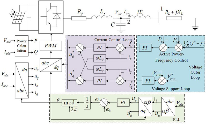
Figure 1. Single Inverter-based Source Single Load System Topology and its Control Structure.

Off-grid renewable energy systems are highly sensitive to environmental conditions, which can cause frequent shifts in operating points. The power balance between the generation and load sides becomes complex and variable under such conditions. As illustrated in Figure 2, certain operating points can maintain frequency stability under small disturbances. However, When the operating point departs substantially from nominal, the system tends to exhibit weakly damped oscillations. Accordingly, developing a frequency-response model with explicitly stated physical mechanisms and enhancing damping via parameter tuning is an effective means to improve the frequency stability of islanded power systems supplied exclusively by converter-interfaced renewable generation.

Figure 2

Figure 2. SFR curves under different operating points.

2.1 Transfer function representation of the inverter frequency response model

The time scale of electromagnetic transients ranges from microseconds to milliseconds, while that of primary frequency control or governor action ranges from several seconds to tens of seconds (Sauer et al., 1997). This paper selects the aforementioned single-machine single-load PV system as the research object, aiming to develop a mathematical model that can accurately and efficiently characterize its frequency stability dynamics. The model is designed to reflect the dynamic response characteristics between the PV output power and the system frequency. Therefore, this paper focuses on the dynamic characteristics of the PV system within the time scale of power system frequency dynamics, which belongs to the slow time scale, ranging from several seconds to tens of seconds. All symbols and units employed in this paper are consistently defined in the Appendix titled “Variable Definition Table.”

For PV panels, under natural conditions, the current-voltage characteristics of the solar panels are primarily influenced by irradiance and temperature. The variations within a time scale of seconds are minimal. Therefore, this paper assumes that the DC voltage output at the terminals of the PV panels remains constant, allowing us to neglect the internal dynamics and model the PV panels as a constant DC voltage source.

For the dual-loop control of current and voltage, the time scale of the inner current loop and the outer voltage loop is typically in the range of tens to hundreds of hertz, which corresponds to a microsecond level, indicating a relatively fast time scale.

For the RLC filter circuit, the time constant is typically used to characterize the settling speed of the circuit. Under typical parameter settings, the time constants of the RC and LC circuits are approximately ${\tau }_{\text{RC}}\approx 1\times {10}^{-6}s$, ${\tau }_{LC}\approx 2.24\times {10}^{-2}s$.

Evidently, the time scale of the RC section involving the filter capacitor is at the microsecond level, which is considered a fast dynamic compared to frequency dynamics.

In summary, the distribution of time scales for various components of the PV system is illustrated in Figure 3. Given that this paper focuses on the frequency response characteristics of the PV system within the slow time scale regime, the subsequent analysis will disregard the fast dynamic components and retain only the power-frequency dynamic characteristics. Specifically, the following assumptions are made to establish the frequency dynamic response model of the PV system: i) Neglect the current inner-loop control at the millisecond to microsecond level, i.e., disregard the transient process of the d-axis current tracking its reference value. ii) Neglect the charging process of the filter capacitor, which occurs on the microsecond timescale. Accordingly, disregard the associated capacitor charging current dynamics in the model.

Figure 3

Figure 3. Time scale of each link in the system.

The simplified components mentioned above are indicated by shaded blocks in Figure 1 to enhance clarity. The linearized state-space model of the inverter-based source system under the frequency-dynamic timescale is provided in Appendix B. In the following sections, the frequency response model of the inverter is derived, with particular emphasis on the dynamic behavior over the time scale relevant to frequency and active power.

For the active power–frequency control section, and utilizing the small-signal model provided in Appendix B, the following transfer function relationships between active power $\Delta P_{\mathrm{e}}$, frequency $\Delta f$, and d-axis current $\Delta i_{\mathrm{d}}$ are established:

$\Delta P_{\mathrm{e}}=-\frac{1}{R}\Delta f-G_{\text{pf}}\Delta i_{\mathrm{d}}(1)$

Where $K_{\mathrm{p}1}$ and $K_{\mathrm{i}1}$ represent the proportional and integral gain, respectively, of the active power-frequency control loop, $R$ represents the droop coefficient, $G_{pf}=\frac{s}{K_{i1}+s{K}_{p1}}$.

To obtain the relationship between active power and frequency in (1), the variable $\Delta i_{\mathrm{d}}$ must be eliminated. By incorporating the definition of inverter output power, the expression of $\Delta P_{\mathrm{e}}$ is introduced to eliminate the voltage and current components at the point of common coupling.

$\Delta P_{\mathrm{e}}=\frac{3}{2}\left(u_{\mathrm{d}0}\Delta i_{\mathrm{d}}+i_{\mathrm{d}0}\Delta u_{\mathrm{d}}+u_{\mathrm{q}0}\Delta i_{\mathrm{q}}+i_{\mathrm{q}0}\Delta u_{\mathrm{q}}\right)(2)$

Where $u_{\mathrm{d}0}$, $i_{\mathrm{d}0}$, $u_{\mathrm{q}0}$ and $i_{\mathrm{q}0}$ represent the steady-state d-axis and q-axis voltages and currents, respectively; $\Delta u_{\mathrm{d}}$, $\Delta i_{\mathrm{d}}$, $\Delta u_{\mathrm{q}}$ and $\Delta i_{\mathrm{q}}$ represent the changes in d-axis and q-axis voltages and currents, respectively.

Due to the introduction of new variables $\Delta u_{\mathrm{q}}$, $\Delta i_{\mathrm{q}}$ and $\Delta u_{\mathrm{d}}$ in Equation 2, it is necessary to eliminate them. First, utilize the linearized expression of the PLL model to eliminate $\Delta u_{\mathrm{q}}$:

$\Delta u_{\mathrm{q}}=G_{\text{pll}}\Delta f(3)$

Where $K_{\mathrm{p}}$ and $K_{\mathrm{i}}$ are the proportional and integral gain, respectively, of the PLL control loop, $G_{\text{pll}}=\frac{2\pi s}{s{K}_{\mathrm{p}}+K_{\mathrm{i}}}$.

Subsequently, combine the grid-side model to eliminate $\Delta i_{\mathrm{q}}$ and $\Delta u_{\mathrm{d}}$. The small-signal model for the line and load is:

$\Delta u_{\mathrm{d}}=R_{\mathrm{L}}\Delta i_{\mathrm{d}}-X\Delta i_{\mathrm{q}}(4)$

$\Delta u_{\mathrm{q}}=R_{\mathrm{L}}\Delta i_{\mathrm{q}}+X\Delta i_{\mathrm{d}}(5)$

Where $X$ represents the sum of the filter inductance, line reactance, and load reactance, while $R_{\mathrm{L}}$ denotes the sum of the filter resistance, line resistance, and load resistance.

By combining Equations 3, 5 the expression for $\Delta i_{\mathrm{q}}$ can be obtained:

$\Delta i_{\mathrm{q}}=G_{\mathrm{L}1}\Delta i_{\mathrm{d}}+G_{\mathrm{L}2}\Delta f(6)$

Where $G_{\mathrm{L}1}=-\frac{X}{R_{\mathrm{L}}}$, $G_{\mathrm{L}2}=\frac{G_{\text{pll}}}{R_{\mathrm{L}}}$.

By substituting Equation 6 into Equation 4 to eliminate $\Delta i_{\mathrm{q}}$, the expression for $\Delta u_{\mathrm{d}}$ can be obtained:

$\Delta u_{\mathrm{d}}=G_{\mathrm{L}3}\Delta i_{\mathrm{d}}-G_{\mathrm{L}4}{G}_{\text{pll}}\Delta f(7)$

Where $G_{\mathrm{L}3}=\frac{R_{\mathrm{L}}^2+X^2}{R_{\mathrm{L}}}$, $G_{\mathrm{L}4}=\frac{X}{R_{\mathrm{L}}}$.

Finally, by substituting Equations 4, 6, 7 into Equation 2, it is possible to eliminate $\Delta u_{\mathrm{q}}$, $\Delta i_{\mathrm{q}}$ and $\Delta u_{\mathrm{d}}$, resulting in an expression for $\Delta P_e$ without introducing new variables:

$\Delta P_{\mathrm{e}}=G_{\mathrm{L}}^{\prime }\Delta i_{\mathrm{d}}+\left(G_{\mathrm{L}}^{‴}-G_{\text{pll}}{G}_{\mathrm{L}}^{″}\right)\Delta f(8)$

Where $G_{\mathrm{L}}^{\prime }=\frac{3}{2}\left(u_{\mathrm{d}0}+i_{\mathrm{d}0}{G}_{\mathrm{L}3}+u_{\mathrm{q}0}{G}_{\mathrm{L}1}\right)=\frac{3}{2}\left(u_{\mathrm{d}0}+i_{\mathrm{d}0}{G}_{\mathrm{L}3}\right)$, $G_{\mathrm{L}}^{″}=\frac{3}{2}\left(i_{\mathrm{d}0}{G}_{\mathrm{L}4}-i_{\mathrm{q}0}\right)$, $G_{\mathrm{L}}^{‴}=\frac{3}{2}{u}_{\mathrm{q}0}{G}_{\mathrm{L}2}=0$.

By substituting Equation 8 into Equation 1, the expression for $\Delta i_d$ can be derived, as shown in Equation 9:

$\Delta i_{\mathrm{d}}=-\frac{-G_{\text{pll}}{G}_{\mathrm{L}}^{″}+G_{\mathrm{L}}^{‴}+\raisebox{1ex}{$1$}\!\left/ \!\raisebox{-1ex}{$R$}\right.}{G_{\text{pf}}+G_{\mathrm{L}}^{\prime }}\Delta f(9)$

By substituting the expression in (9) into (1), the transfer function form of the inverter-based SFR model is obtained. This model effectively characterizes the dynamic interaction between inverter active power and system frequency.

$\Delta P_{\mathrm{e}}=\left[\frac{-R{G}_{\text{pf}}{G}_{\text{pll}}{G}_{\mathrm{L}}^{″}-G_{\mathrm{L}}^{\prime }}{R\left(G_{\text{pf}}+G_{\mathrm{L}}^{\prime }\right)}\right]\Delta f(10)$

Equation 10 establishes a reduced-order, physically interpretable frequency response model for inverter-based source. In comparison with the full electromagnetic transient model, this formulation reduces computational complexity while preserving the essential frequency dynamics. The physical interpretability originates from its derivation based on inverter control dynamics rather than empirical fitting, with model parameters directly corresponding to measurable physical quantities. Consequently, the model elucidates the intrinsic mechanism by which active power disturbances influence frequency stability.

2.2 Block diagram representation of the inverter-based frequency response model

Equation 10 defines the SFR model of the inverter in the transfer function domain. This model captures the dynamic interactions among the active power–frequency control loop, the line and load subsystem, and the PLL. Based on the mathematical formulations in (1), (2), (4), and (7), the corresponding block diagram representation of the inverter-based SFR model is constructed, as illustrated in Figure 4.

Figure 4

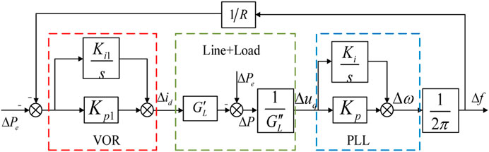
Figure 4. SFR block diagram of inverter-based source reflecting frequency response process.

Compared with the transfer function-based SFR model presented in Section 2.1, the block diagram model shown in Figure 4 provides clearer insight into the physical mechanism underlying the inverter’s frequency response. When an active power disturbance $\Delta P_{\mathrm{e}}$ occurs, the response begins with the inverter’s outer voltage control loop, which performs active power–frequency regulation. This loop employs a proportional–integral (PI) controller to adjust the inverter’s active current $\Delta i_{\mathrm{d}}$, thereby modulating the inverter’s active power output to help restore the system frequency. The regulated current $\Delta i_{\mathrm{d}}$ is then injected into the inverter’s grid-side network, where it interacts with the impedance characteristics of the transmission line and load. As a result, the quadrature-axis terminal voltage $\Delta u_{\mathrm{q}}$ changes and is fed into the PLL. The PLL processes $\Delta u_{\mathrm{q}}$ to yield the frequency deviation $\Delta f$ ,which is subsequently fed back to the outer voltage control loop. This forms a closed-loop interaction that captures the dynamic coupling between the inverter and system frequency.

Meanwhile, the aforementioned inverter frequency response process reveals the dynamic interaction mechanism between the inverter’s active power and the system frequency. Specifically, when a disturbance causes a frequency deviation $\Delta f$, this deviation is fed into the inverter’s active power–frequency droop control, which accordingly adjusts the active power reference value ${\mathrm{P}}_{\mathrm{r}ef}$. On the inverter side, the updated ${\mathrm{P}}_{\mathrm{r}ef}$ is processed sequentially through three cascaded modules—namely, the outer power control loop, the line-load impedance dynamics, and the PLL. This sequence of dynamic responses collectively exerts a feedback effect on the evolution of the system frequency deviation $\Delta f$.

In summary, the inverter SFR block diagram model proposed in this paper offers a significant advantage in revealing the dynamic process through which renewable energy systems participate in system frequency response. This is because the model is derived analytically based on the mathematical representations and interrelations of key physical components of the inverter on the frequency-dynamic timescale, resulting in a physically interpretable SFR formulation. In contrast, the singular perturbation method directly separates the fast and slow dynamics of the system through mathematical techniques, which may compromise the structural physical interpretability of the SFR model during matrix inversion. Moreover, improper selection of model order or parameters may lead to the omission of critical dynamic characteristics. As for data-driven machine learning algorithms, their decision-making processes are primarily based on statistical correlations in historical data rather than fundamental physical laws, often leading to a “black-box” nature. Consequently, such models generally lack transparency and are unable to provide clear physical insight into system behavior.

3 Parameter identification of the inverter frequency response model

This section focuses on the parameter identification methods for both the mathematical and block diagram representations of the inverter frequency response model. First, analytical expressions for the dynamic performance indices of the SFR model are derived to formulate the parameter identification framework for the inverter’s transfer function and block diagram models. Subsequently, a parameter estimation approach based on the Levenberg–Marquardt algorithm is proposed for solving the identification problem.

3.1 Parameter identification model of the inverter SFR transfer function

The transfer function form of the inverter SFR model has been provided in Equation 10. By substituting the parameters $G^{\prime }$, $G_L^{″}$, and $G_L^{‴}$ into Equation 10 and performing algebraic simplification, the inverter SFR model can be expressed in the following standard second-order form:

$\frac{\Delta f}{\Delta P_{\mathrm{e}}}=\frac{a_0+a_{1}s+a_2{s}^2}{b_0+b_{1}s+b_2{s}^2}(11)$

Where $a_0$, $a_1$, $a_2$, $b_0$, $b_1$, and $b_2$ are the parameters to be identified in the inverter SFR transfer function model.

To further ensure the model’s interpretability and parameter traceability, a physically-based description is adopted. A physically-based model is defined as one in which the parameters possess explicit physical meanings. In the proposed SFR model, the coefficients ${\mathrm{a}}_0,{\mathrm{a}}_1,{\mathrm{a}}_2,{\mathrm{b}}_0,{\mathrm{b}}_1,{\mathrm{b}}_2$ are not abstract number but are directly linked to the controller parameters, line impedance, filter parameters and load impedance. When the control parameters vary, these coefficients are correspondingly updated, forming an inherent relationship between the control law and the model parameters. The proposed SFR model establishes an explicit physical mapping between its parameters and controller quantities, ensuring interpretability.

Based on this formulation, the dynamic characteristics of the inverter SFR model are quantitatively analyzed. By performing the inverse Laplace transform, the time-domain response of Equation 11 to a unit step disturbance can be derived as follows:

$c\left(t\right)=\frac{a_0}{b_0}+\frac{\mathrm{\Upsilon }}{b_0}{e}^{-\zeta {\omega }_{\mathrm{n}}t}\cos \left({\omega }_{\mathrm{d}}t-{\mathrm{\Lambda }}_1\right)(12)$

Where ${\omega }_{\mathrm{d}}$ represents the damped natural frequency, ${\mathrm{{\rm X}}}_2=\left(a_1{\omega }_{\mathrm{n}}-a_2{\omega }_{\mathrm{n}}^2\zeta -a_0\zeta \right)/\sqrt{1-{\zeta }^2},{\mathrm{{\rm X}}}_1=a_2{\omega }_{\mathrm{n}}^2-a_0,{\omega }_{\mathrm{n}}=\sqrt{b_0/b_2},\zeta =b_1/2\sqrt{b_0{b}_2},{\mathrm{\Lambda }}_1=t{g}^{-1}{\mathrm{{\rm X}}}_2/{\mathrm{{\rm X}}}_1,\mathrm{\Upsilon }=\left|{\mathrm{{\rm X}}}_1+j{\mathrm{{\rm X}}}_2\right|,{\omega }_{\mathrm{d}}=\sqrt{1-{\zeta }^2}{\omega }_{\mathrm{n}}$, ${\omega }_{\mathrm{n}}$ represents the undamped natural frequency of the system.

Based on the time-domain expression in Equation 12, the key dynamic performance metrics of the inverter SFR model under step response can be sequentially derived, including peak time $t_{\mathrm{p}}$, peak value $c\left(t_{\mathrm{p}}\right)$, overshoot $\Delta p$, and rise time $t_{\mathrm{r}}$.

The peak time refers to the time required for the response to reach its first peak after exceeding the steady-state value. According to its definition, the peak time $t_{\mathrm{p}}$ is determined as the time at which the first derivative of Equation 13 becomes zero. Therefore, it can be expressed as follows:

$t_{\mathrm{p}}=\left(0.5\pi +{\mathrm{\Lambda }}_1+{\mathrm{\Lambda }}_2\right)/{\omega }_{\mathrm{d}}(13)$

Where ${\mathrm{\Lambda }}_2=t{g}^{-1}\sqrt{1-{\zeta }^2}/\zeta$.

The peak value $c\left(t_{\mathrm{p}}\right)$ can be obtained by substituting $t_{\mathrm{p}}$ into Equation 12, from which Equation 14 is derived.

$c\left(t_{\mathrm{p}}\right)=\frac{a_0}{b_0}+\frac{\mathrm{\Upsilon }}{b_0}{e}^{-\frac{\zeta }{\sqrt{1-{\zeta }^2}}\left(\left(0.5\pi +{\mathrm{\Lambda }}_1+{\mathrm{\Lambda }}_2\right)\right)}\cos \left(0.5\pi +{\mathrm{\Lambda }}_2\right)(14)$

The overshoot is an index used to quantify the extent to which the system response exceeds its final steady-state value. It is defined as the ratio of the deviation between the peak value $c\left(t_{\mathrm{p}}\right)$ and the steady-state value $c\left(\infty \right)$ to the steady-state value, as shown in Equation 15.

$\Delta p=\frac{c\left(t_{\mathrm{p}}\right)-c\left(\infty \right)}{c\left(\infty \right)}\times 100\%(15)$

From the analysis of the inverter’s unit step response in Equation 13, the steady-state value $c\left(\infty \right)$ can be determined. This response comprises two components: a constant term $\frac{a_0}{b_0}$, and a transient term that decays exponentially with time as governed by the parameter $e^{-\zeta {\omega }_{\mathrm{n}}t}$. As time approaches infinity, the transient term vanishes, leaving the steady-state value as $c\left(\infty \right)=\frac{a_2}{b_2}$. Substituting $c\left(t_{\mathrm{p}}\right)$ and $c\left(\infty \right)$ into Equation 16 yields:

$\Delta p=\frac{\mathrm{\Upsilon }}{a_0}{e}^{-\frac{\zeta }{\sqrt{1-{\zeta }^2}}\left(\left(0.5\pi +{\mathrm{\Lambda }}_1+{\mathrm{\Lambda }}_2\right)\right)}\cos \left(0.5\pi +{\mathrm{\Lambda }}_2\right)(16)$

The rise time refers to the duration required for the response curve to increase from 10% to 90% of its steady-state value. For computational simplicity, $t_r$ is defined as the time at which the response $c\left(t_{\mathrm{r}}\right)$ first reaches the steady-state value $c\left(\infty \right)$, and its expression is derived as shown in Equation 17.

$t_{\mathrm{r}}=\left(0.5\pi +{\mathrm{\Lambda }}_1\right)/{\omega }_{\mathrm{d}}(17)$

The analytical expressions for the four dynamic performance indices have thus been derived. However, since the number of unknown parameters in Equation 11 exceeds the number of available performance indices, these parameters cannot be directly solved. Consequently, an optimization model is formulated in the following section to estimate the parameters of Equation 11.

An effective approach to evaluate whether the identified parameters of the inverter-based SFR transfer function model are satisfactory is to compare the model’s response with measured data. Accordingly, the following objective function is established:

$\min F=\frac{1}{n}{\displaystyle \sum _{i=1}^n}{\left(c_{\mathrm{i}}\left(k\right)-c_{\text{mi}}\left(k\right)\right)}^2(18)$

In the equation, $c_{\text{mi}}\left(k\right)$ represents the value of the $i$ measured disturbance response sample at time $k$, while $c_{\mathrm{i}}\left(k\right)$ denotes the corresponding theoretical value at time $k$ obtained from Equation 11 using the current parameter set. The objective function is defined as the average over $n$ samples to mitigate the influence of measurement noise from any individual sample.

When the SFR model of the inverter-based source is identified with an optimal set of parameters, the theoretical values of dynamic performance indices calculated from Equation 13 through Equation 17 will closely match the corresponding measured values. Based on this principle, constraint conditions are formulated in this section to ensure consistency between the theoretical and measured dynamic characteristics:

$\left\{\begin{array}{l}{t}_{\mathrm{p},\mathrm{m}}=t_{\mathrm{p}}\\ c_{\mathrm{m}}\left(t_{\mathrm{p}}\right)=c\left(t_{\mathrm{p}}\right)\\ \Delta p_{\mathrm{m}}=\Delta p\\ t_{\mathrm{r},\mathrm{m}}=t_{\mathrm{r}}\end{array}\right.(19)$

Where $t_{\mathrm{p},\mathrm{m}}$, $c_{\mathrm{m}}\left(t_{\mathrm{p}}\right)$, $\Delta p_{\mathrm{m}}$, and $t_{\mathrm{r},\mathrm{m}}$ represent the measured values of peak time, peak value, overshoot, and rise time obtained from the disturbance response curve, respectively. $t_{\mathrm{p}}$, $c\left(t_{\mathrm{p}}\right)$, $\Delta p$, and $t_{\mathrm{r}}$ denote the corresponding theoretical values computed by substituting the current model parameters into Equation 13 through Equation 18.

Accordingly, the parameter optimization framework for the inverter-based SFR transfer function model is established by combining the objective function defined in Equation 18 with the constraint conditions specified in Equation 19. When a particular set of parameters minimizes the objective function below a predefined error threshold, it is regarded as yielding a satisfactory and physically meaningful representation of the inverter’s SFR characteristics.

3.2 Parameter optimization model of the inverter SFR block diagram

Although Section 3.1 provides a solution to the transfer function representation of the inverter SFR model, the resulting expression reflects only the overall response of all internal control and system components combined. The specific parameters associated with the key internal control loops of the inverter remain unidentified. Therefore, based on the results from Section 3.1, this subsection further develops an optimization model for the inverter SFR block diagram as shown in Figure 4.

By deriving the parameter expressions of the inverter SFR model from Equation 10 and comparing them with Equation 11, the following set of equality relationships can be established between the parameters of the inverter SFR transfer function model and those of the SFR block diagram model, as presented in Section 3.2:

$\left\{\begin{array}{l}{a}_0=R{K}_{\mathrm{p}}+R{K}_{\mathrm{p}}{K}_{\mathrm{p}1}{G_{\mathrm{L}}}^{\prime }\\ a_1=R{K}_{\mathrm{i}}+R{K}_{\mathrm{p}}{K}_{\text{il}}{G_{\mathrm{L}}}^{\prime }+R{K}_{\mathrm{i}}{K}_{\mathrm{p}1}{G_{\mathrm{L}}}^{\prime }\\ a_2=R{K}_{\mathrm{i}}{K}_{\text{il}}{G_{\mathrm{L}}}^{\prime }\\ b_0=-2\pi {G_{\mathrm{L}}}^{″}R-K_{\mathrm{p}}{K}_{\mathrm{p}1}{G_{\mathrm{L}}}^{\prime }\\ b_1=-K_{\mathrm{i}}{K}_{\mathrm{p}1}{G_{\mathrm{L}}}^{\prime }+K_{\mathrm{p}}{K}_{\text{il}}{G_{\mathrm{L}}}^{\prime }\\ b_2=-K_{\mathrm{i}}{K}_{\text{il}}{G_{\mathrm{L}}}^{\prime }\end{array}\right.(20)$

By substituting Equation 20 into Equation 13 through Equation 17, the objective function defined in Equation 19 and the constraint conditions specified in Equation 18 can be reformulated in terms of the system parameters of the inverter SFR block diagram model. Consequently, the parameter optimization model established in Section 3.1 is transformed into an optimization framework aimed at identifying the parameters of the inverter SFR block diagram model.

3.3 Optimization method

Sections 3.1, 3.2 respectively formulate parameter optimization models for the inverter-based source SFR transfer function and block diagram models. To obtain the optimal solutions of these models, this section presents an optimization approach based on the Levenberg–Marquardt method.

The core idea of the Levenberg–Marquardt method lies in introducing a damping factor $\lambda$ to combine the update rules of the Gauss–Newton method with those of the gradient descent method. When the error is small, the damping factor is reduced, making the algorithm behave more like the Gauss–Newton method, thereby accelerating convergence. Conversely, when the error is large or the step size is inappropriate, the damping factor is increased, causing the algorithm to lean toward gradient descent, thus enhancing stability. The Jacobian matrix $J$ of the objective function is computed to reflect the error gradient, as shown in Equation 21.

$J_{\text{ij}}=\frac{\mathrm{\partial }{F}_{\mathrm{i}}}{\mathrm{\partial }{\gamma }_{\mathrm{j}}}(21)$

Where $F_{\mathrm{i}}$ represents the $i$ dynamic performance index, and ${\gamma }_{\mathrm{j}}$ denotes the $j$ parameter to be estimated.

To achieve both stability and fast convergence, the Levenberg–Marquardt method modifies the classical Gauss–Newton algorithm by incorporating a damping term. This augmentation allows the algorithm to behave like the Gauss–Newton method when the error is small and like the gradient descent method when the error is large, thereby improving robustness. The parameter ${\gamma }_{k+1}$ update expression is formulated as follows:

${\gamma }_{\mathrm{k}+1}={\gamma }_{\mathrm{k}}-{\left[J{\left({\gamma }_{\mathrm{k}}\right)}^{T}J\left({\gamma }_{\mathrm{k}}\right)+\lambda I\right]}^{-1}J{\left({\gamma }_{\mathrm{k}}\right)}^{T}r\left({\gamma }_{\mathrm{k}}\right)(22)$

Where $I$ denotes the identity matrix and $\lambda$ is the damping factor, which is dynamically adjusted based on the variation of the objective function. Specifically, if the objective function value decreases, $\lambda$ is reduced to allow a larger step size, thereby accelerating convergence. Conversely, if the objective function value increases, $\lambda$ is increased to reduce the step size, enhancing stability. This adaptive adjustment enables the algorithm to converge robustly when the initial estimate is far from the true solution and to converge rapidly when the estimate is near the optimal point. The vector $r\left({\gamma }_k\right)$ represents the residuals, as shown in Equation 23.

$\begin{array}{l}r\left({\gamma }_{\mathrm{k}}\right)=\frac{1}{n}\left[\begin{array}{cc}{\displaystyle \sum _{i=1}^n}\left(t_{\mathrm{p},\text{mi}}-t_{\text{pi}}\right)& {\displaystyle \sum _{i=1}^n}\left(c_{\text{mi}}\left(t_{\mathrm{p},\text{mi}}\right)-c_{\mathrm{i}}\left(t_{\text{pi}}\right)\right)\end{array}\right.\\ {\left.{\displaystyle \sum _{i=1}^n}\left(\Delta p_{\text{mi}}-\Delta p_{\mathrm{i}}\right){\displaystyle \sum _{i=1}^n}\left(t_{\mathrm{r},\text{mi}}-t_{\text{ri}}\right)\right]}^T\end{array}(23)$

The iteration terminates either upon reaching the maximum number of iterations or when the following convergence criterion is satisfied, as shown in Equation 24.

$\left\{\begin{array}{l}F<{\epsilon }_2\\ \max r\left({\gamma }_{\mathrm{k}}\right)<{\epsilon }_1\end{array}\right.(24)$

Where ${\epsilon }_1$ and ${\epsilon }_2$ represent the thresholds for the residual and the objective function, respectively.

The inverter SFR model can be obtained using the aforementioned Levenberg–Marquardt algorithm, and its flowchart is shown in Figure 5.

Figure 5

Figure 5. Parameters identification flowchart for inverter-based source SFR model.

Firstly, initial estimates of the parameters in the SFR transfer function model are assigned. These values are substituted into Equation 13 through Equation 17 to compute the predicted dynamic performance indices. Based on the measured peak time, peak value, overshoot, and rise time obtained from the disturbance response curves, the initial value of the objective error function is calculated using Equation 18. The Jacobian matrix is then employed to evaluate the error gradient, and the parameters are updated according to Equation 22 to obtain a new estimate denoted ${\gamma }_{\mathrm{k}+1}$.

Then, the updated parameter set ${\gamma }_{\mathrm{k}+1}$ is re-substituted into the objective function. If the new parameter set ${\gamma }_{\mathrm{k}+1}$ results in a reduced objective function value, the update is accepted and the damping factor is decreased. Otherwise, the update is rejected and the damping factor is increased.

Finally, the algorithm checks whether the maximum number of iterations has been reached or whether the convergence criteria are satisfied. If either condition is met, the iterative process is terminated. Otherwise, the above steps are repeated. Through this iterative procedure, the optimal values of the inverter SFR transfer function parameters $a_0$, $a_1$, $a_2$, $b_0$, $b_1$, and $b_2$ can be effectively identified.

Since the procedure for estimating the optimal parameters of the inverter SFR block diagram model mirrors that of the transfer function model, it is not reiterated here for conciseness.

4 Applications of the inverter SFR model

Due to the inherent relationship described in Section 3.1, two important properties can be derived. First, when the operating point changes, the model can be automatically updated without complex recalculations. Second, when an operating-point shift causes insufficient damping, the damping ratio derived from the transfer function allows direct online adjustment through parameter tuning. The following sections, 4.1 and 4.2, respectively elaborate on these two properties in detail.

4.1 Online updating strategy of the SFR model

Subject to source–load power fluctuations, the operating point may shift, and the SFR model of the inverter identified at the original operating point may no longer be valid under the new operating condition. To ensure frequency stability, this paper proposes an online updating strategy that adopts the system critical inertia (Yang et al., 2024) as the triggering criterion. When the actual system inertia falls below the critical inertia threshold, it indicates a potential inability to maintain frequency stability. In such cases, the online updating strategy is activated to correct the model parameters.

Firstly, the inverter system parameters obtained using the method presented in Section 2 are extracted. Then, based on the PMU measurements of the inverter’s active power output $P_{\text{new}}$ and the load-side voltage $U_{\text{new}}$ under the current operating condition, the steady-state values of the system state variables $i_{d0}$, $i_{q0}$, $u_{d0}$, $u_{q0}$ at the new operating point are computed according to Equation 25.

$\left\{\begin{array}{l}{i}_{\mathrm{d}0\_\text{new}}{R}_{\mathrm{L}}-i_{\mathrm{q}0\_\text{new}}X=U_{\text{new}}\\ i_{\mathrm{q}0\_\text{new}}{R}_{\mathrm{L}}+i_{\mathrm{d}0\_\text{new}}X=0\\ 1.5*\left(u_{\mathrm{d}0\_\text{new}}{i}_{\mathrm{d}0\_\text{new}}+u_{\mathrm{q}0\_\text{new}}{i}_{\mathrm{q}0\_\text{new}}\right)=P_{\text{new}}\end{array}\right.(25)$

The steady-state values of the state variables and the control system parameters are substituted into Equation 20 to calculate the SFR model parameters under the current operating condition. This process updates the SFR model to match the new operating point. The complete procedure of the online updating strategy is shown in Figure 6.

Figure 6

Figure 6. Update flowchart for SFR model online updating.

4.2 Enhancement strategy of online inertia and damping

This section proposes an online enhancement strategy for the inertia and damping of inverter-based source system. The baseline control parameters are designed to ensure frequency stability under small disturbances around the nominal operating point. However, when the operating point undergoes significant deviations, these baseline parameters may no longer be adequate. To ensure sufficient inertia and damping at the new operating point, this strategy adjusts the inverter control parameters in real time.

When the system’s inertia and damping fall below the minimum threshold required for secure and stable operation, an online parameter adjustment strategy is triggered. The triggering condition is defined as follows:

${\mathrm{\Gamma }}_{\mathrm{J}}<{{\mathrm{\Gamma }}_{\mathrm{J}}}_{\text{threshold}}or{\mathrm{\Gamma }}_{\mathrm{D}}<{{\mathrm{\Gamma }}_{\mathrm{D}}}_{\text{threshold}}(26)$

Where ${\mathrm{\Gamma }}_{\mathrm{J}}$ and ${\mathrm{\Gamma }}_{\mathrm{D}}$ represent the evaluated indices of inertia and damping, respectively. ${{\mathrm{\Gamma }}_{\mathrm{J}}}_{\text{threshold}}$ and ${{\mathrm{\Gamma }}_{\mathrm{D}}}_{\text{threshold}}$ denote the corresponding minimum threshold values for system stability.

Efficient enhancement of system inertia and damping hinges on appropriate selection of control parameters. To achieve this, sensitivity analysis is conducted to compare how different parameters influence inertia and damping. The parameter with the highest sensitivity is chosen for adjustment. Sensitivity is defined as shown in Equation 27.

$\left\{\begin{array}{l}{\gamma }_x=\frac{\mathrm{\partial }{\mathrm{\Gamma }}_{\mathrm{J}}}{\mathrm{\partial }x}\\ {\eta }_x=\frac{\mathrm{\partial }{\mathrm{\Gamma }}_{\mathrm{D}}}{\mathrm{\partial }x}\end{array}\right.(27)$

Where ${\gamma }_x$ and ${\eta }_x$ represent the sensitivities of the inertia and damping indices with respect to different control parameters, and $x$ denotes the control parameter. The sensitivity values are obtained numerically, with a small perturbation magnitude defined as $\Delta x\%=\Delta x/x_0$.

Considering the discrepancy between the inertia and damping indices of the SFR model after parameter optimization and their target values, the objective function is formulated as follows:

$\min \left[\left({\mathrm{\Gamma }}_{\mathrm{J}}-{{\mathrm{\Gamma }}_{\mathrm{J}}}_{\text{opt}}\right)+\left({\mathrm{\Gamma }}_{\mathrm{D}}-{{\mathrm{\Gamma }}_{\mathrm{D}}}_{\text{opt}}\right)\right](28)$

Where ${\mathrm{\Gamma }}_{\text{Jopt}}$ and ${\mathrm{\Gamma }}_{\text{Dopt}}$ represent the target values of ${\mathrm{\Gamma }}_{\mathrm{J}}$ and ${\mathrm{\Gamma }}_{\mathrm{D}}$, respectively.

To realize the online enhancement strategy for inertia and damping, the analytically derived SFR model is utilized. The oscillation frequency and damping ratio of the system’s frequency oscillation mode are adopted as the inertia and damping indices, denoted as indicators ${\mathrm{\Gamma }}_{\mathrm{J}}$ and ${\mathrm{\Gamma }}_{\mathrm{D}}$, respectively.

$\left\{\begin{array}{l}{\mathrm{\Gamma }}_{\mathrm{J}}=\frac{\beta }{2\pi }\\ {\mathrm{\Gamma }}_{\mathrm{D}}=-\frac{\alpha }{\sqrt{{\alpha }^2+{\beta }^2}}\end{array}\right.(29)$

Where $p=\alpha \pm j\beta$ denotes the poles of the SFR model.

The workflow of the online inertia and damping enhancement strategy is illustrated in Figure 7. First, the current system inertia and damping indicators are calculated using Equation 29, and evaluated against the trigger condition defined in Equation 26. If either indicator falls below its respective threshold, the system enters the parameter optimization procedure. Subsequently, the sensitivities of the inertia and damping indicators with respect to all control parameters are computed. The control parameter with the largest absolute sensitivity is selected as the optimization variable, and its adjustment direction is determined by the sign of the sensitivity. Finally, an objective function is constructed to minimize the deviation between the inertia and damping indicators of the SFR model and their target values. The optimal adjustment of the selected control parameter is then obtained using the Levenberg–Marquardt algorithm.

Figure 7

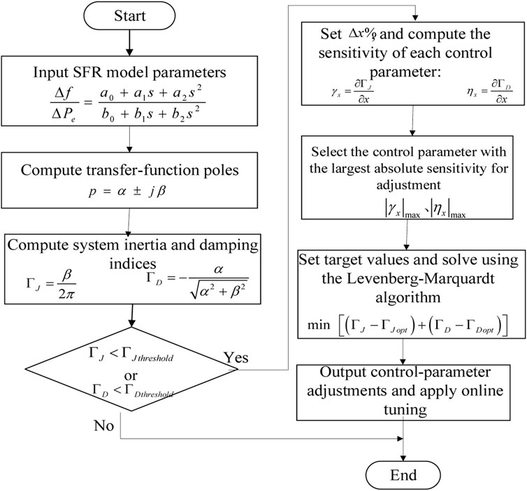
Figure 7. Flowchart for inertia and damping online improvement.

5 Simulation analysis

This section presents validation and analysis to assess the accuracy of the proposed inverter frequency response model, the feasibility of the parameter identification method, and the effectiveness of the model’s application.

5.1 Validation of the inverter SFR model

5.1.1 Accuracy of the inverter SFR model

A comparison is conducted between the SFR model of the inverter-based source proposed in this paper and the detailed model developed in MATLAB/Simulink. The Simulink model is constructed based on the system diagram and control structure illustrated in Figure 1, while the proposed model is built according to Equation 10 and the block diagram shown in Figure 4. Relevant system parameters are listed in Appendix C. To evaluate the model under various power disturbances, the following test scenario is considered: the load side experiences successive disturbances denoted as $\Delta P_{\mathrm{L}1}=+0.2 p.u.$ and $\Delta P_{\mathrm{L}2}=-0.1 p.u$, and the results are shown in Figure 8.

To further verify the applicability and robustness of the proposed SFR model under varying operating conditions, simulations were conducted not only under the aforementioned active power step disturbance but also across multiple steady-state operating points. As the load level changes, the system’s steady-state operating point shifts accordingly, leading to variations in the dynamic characteristics of inverter-based power sources. To overcome the limitation of model validation at a single operating point and to enhance the overall adequacy and reliability of the assessment, identification and comparison tests were carried out at 100 distinct operating points.

For each operating point, the system’s frequency response data were extracted for parameter identification to establish the corresponding second-order SFR model. The output of the identified model was then compared with the electromagnetic transient simulation results at the same operating point. To analyze the differences between the two frequency response curves, the root mean square error (RMSE) was calculated, as shown in the following equation.

$\text{RMSE}=\sqrt{\frac{1}{\mathrm{N}}{\displaystyle \sum _{\mathrm{i}=1}^{\mathrm{N}}}{\left({\mathrm{f}}_{\mathrm{i}}-{\widehat{\mathrm{f}}}_{\mathrm{i}}\right)}^2}(30)$

where $N$ represents the total number of sampling points, $f_i$ denotes the frequency value obtained from the SFR model at the $i$-th sampling point, and $\widehat{f_i}$ denotes the corresponding frequency value from the electromagnetic transient simulation.

The RMSE results for all operating points were then subjected to probabilistic statistical analysis, and the probability density distribution of the errors was plotted, as shown in Figure 9. Smaller RMSE values indicate that the SFR model output closely matches the electromagnetic transient simulation results, demonstrating high model accuracy across different operating points. The RMSE values approximately follow a normal distribution centered around 0.0034 Hz, with most samples distributed within the range of 0.002 Hz–0.005 Hz. This indicates that the model errors are small and mainly caused by random fluctuations rather than systematic bias.

Figure 8

Figure 8. Comparison of frequency response curves under active power disturbance. (a) $\Delta P_{\mathrm{L}1}=+0.2p.u.$ (b) $\Delta P_{\mathrm{L}2}=-0.1p.u.$

Figure 9

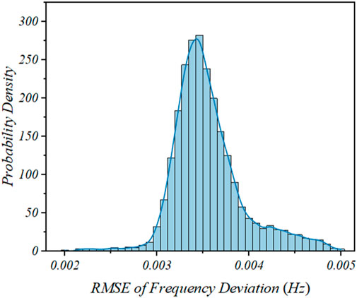
Figure 9. Probability density distribution of RMSE values for 100 operating points.

Overall, the established second-order SFR model accurately reproduces the system’s dynamic frequency response characteristics during both transient and settling periods, exhibiting good applicability and robustness under various operating conditions.

5.1.2 Validation of inverter SFR model order

A reduced second-order frequency response model is derived from the 12th-order full-order mathematical model of the inverter, as expressed in Equation 28.

If further model order reduction is considered by neglecting the PI control loop of the outer voltage controller, a first-order frequency response model (Model 2) can be obtained. Taking the detailed model as the reference, a comparison between the proposed second-order model (Model 1) and the first-order model (Model 2) is conducted. The simulation results are presented in Figure 10.

Figure 10

Figure 10. Comparison of frequency response curves of different model orders.

As shown in Figure 10, the proposed second-order model (Model 1) provides accurate representation of the frequency dynamics within the 0.1 s–1 s time range. Its performance closely matches the detailed model. The slight differences arise from the simplifications made during model reduction, where fast-scale components such as filter capacitor current and inner-loop current reference were neglected. These small deviations are acceptable for analyzing frequency dynamic characteristics. In contrast, although Model 2 further reduces the model order, its accuracy declines over time. From the beginning of the simulation, frequency deviation gradually accumulates. Around 0.15 s, the deviation increases significantly, leading to a failure in capturing the system’s frequency behavior. As a result, Model 2 becomes unsuitable for frequency dynamics analysis.

To further verify the dynamic accuracy of the proposed model, a third-order inverter SFR model was additionally established in Simulink for comparative analysis. Under the active power step disturbance of $\Delta P_{\mathrm{L}2}=-0.1p.u.$, the frequency response curves of the proposed second-order SFR model, the electromagnetic transient simulink, and the third-order SFR model were extracted and compared, as shown in Figure 11.

Figure 11

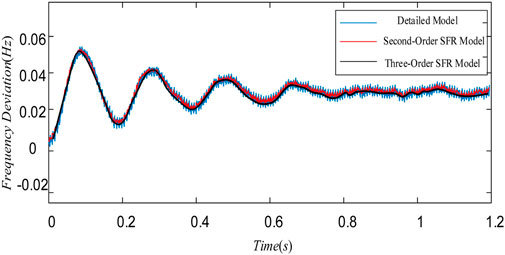
Figure 11. Comparison of different-order SFR and electromagnetic transient model responses.

The results show that the third-order model and the proposed second-order SFR model are both highly consistent with the electromagnetic transient model, with their frequency response curves almost completely overlapping on the dynamic time scale. Although the proposed model retains only a second-order dynamic structure, it demonstrates excellent agreement with the electromagnetic transient simulation results in both response amplitude and timing, accurately capturing the dominant frequency dynamics of the inverter system.

Compared with the third-order model, the proposed second-order SFR model achieves nearly identical dynamic accuracy while requiring fewer parameters and reduced computational complexity. This indicates that the second-order model can effectively reproduce the essential dynamic characteristics of the system without sacrificing precision. Considering both model complexity and accuracy requirements, the proposed model attains an optimal balance between simplicity and fidelity.

In summary, this analysis confirms that the proposed second-order SFR model reaches the practical limit of model order reduction. It represents the lowest valid order capable of maintaining high accuracy while minimizing system complexity, effectively capturing the key frequency response behavior of inverter-based systems.

5.2 Validation of inverter SFR model parameter identification

5.2.1 Accuracy of the parameter identification method

Based on the parameter optimization approach presented in Section 3, the identification process was carried out following the flowchart shown in Figure 5. The resulting inverter SFR model coefficients are listed under the “Close Initial Guess” column in Table 1. The identification process took 0.2306 s, and convergence of optimization error is shown in Figure 12.

Table 1

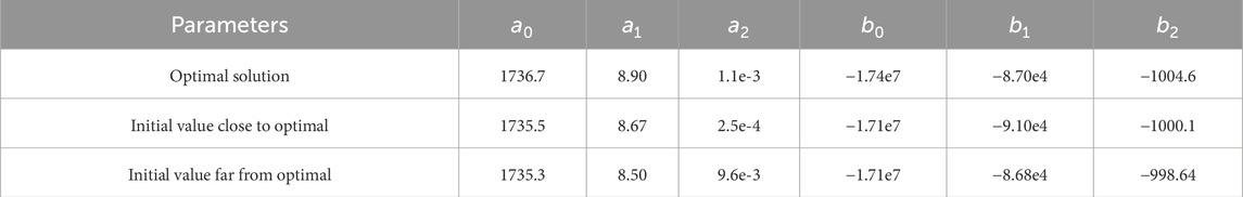
Table 1. Identified results under different initial parameters.

Figure 12

Figure 12. Error convergence in parameter identification process.

To validate the identified model, the parameters obtained from the identification process were substituted into the proposed SFR model. A comparative analysis was then conducted between the model’s response and the electromagnetic transient simulation results. As shown in Figure 13, under the same active power step disturbance, the identified model’s response curve closely matches the observed signal from the electromagnetic transient simulation. The discrepancies in response time and overshoot are both less than 0.1%. These results demonstrate that the identified model exhibits high accuracy and effectively captures the actual frequency dynamics of the system.

Figure 13

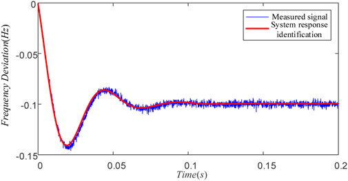
Figure 13. Comparison of the electromagnetic transient simulation signal and the response of the identified SFR model.

To investigate the impact of initial parameter values on the convergence performance of the identification method, this study compares the identified parameters obtained from initial values that are either close to or far from the optimal solution. Based on comparative experiments, the identification results are summarized in Table 1. Under both “near” and “far” initial settings, all parameters effectively converge to the vicinity of the optimal solution. The relative errors of the parameters range from 0.08% to 4.49%, with an average of approximately 1.9%, all within a narrow margin. These results indicate that the proposed method maintains high accuracy and stability even when the initial estimates deviate from the optimum, thereby demonstrating strong robustness.

Substituting both sets of identified parameters into the SFR model, responses under the same active power step disturbance were tested. As shown in Figure 14, identified model responses closely match observed signals. Errors in response time and overshoot remain below 0.1%. This confirms that the proposed identification method effectively approaches optimal parameters and ensures stable convergence even when initial estimates are far from true values.

Figure 14

Figure 14. Comparison of response curves of identified models with initial values far from and close to true values.

To further verify the applicability and robustness of the proposed method under different disturbance conditions, additional simulations were carried out. Taking an impulse disturbance as an example, when the system was subjected to a power impulse, the proposed LM-based identification method was applied to obtain a new set of parameters. These parameters were then substituted into the SFR model to evaluate its response under active power impulse conditions. The results were compared with the electromagnetic transient simulation, as shown in the figure.

As shown in Figure 15, the SFR model under impulse disturbance closely matches the electromagnetic transient simulation results. The main discrepancies appear around the first trough and the subsequent small overshoot, where slight amplitude and timing deviations are observed. Afterward, the two curves converge rapidly without any noticeable steady-state bias. Overall, the identified model effectively captures the main dynamic characteristics of the electromagnetic transient response, such as the rise, peak, and settling processes, demonstrating that the proposed model maintains good applicability and robustness under impulse disturbance conditions.

Figure 15

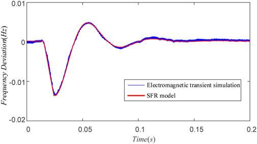
Figure 15. Comparison of frequency response curves under impulse disturbance.

5.2.2 Cramér-Rao bound estimation

This section first derives the Cramér-Rao Lower Bound (CRLB) by computing the Fisher Information Matrix and applying the Cramér-Rao inequality. The CRLB represents the theoretical lower bound on the variance of any unbiased estimation method, serving as the minimum achievable variance for identified parameters. Subsequently, under multiple sets of measured response data, a series of identified parameter groups are obtained. Monte Carlo simulation is then employed to perform statistical analysis on all identified parameter sets, allowing the variance of each estimated parameter to be computed. Finally, the variances obtained from Monte Carlo simulations are compared with the CRLB to evaluate the estimation performance of the proposed identification method.

Following the aforementioned procedure, the identification performance of the method illustrated in Figure 5 was evaluated based on the inverter model. As shown in Figure 16, the estimated variances of the six parameters were only marginally higher than the CRLB, with average ratios between 1.23 and 1.6, thereby confirming the validity of the proposed identification method. Moreover, consistent results obtained with both near-optimal and substantially deviated initial estimates indicate that the method possesses robust convergence characteristics.

Figure 16

Figure 16. Comparison of estimated variance and CRLB for each parameter.

5.3 Application of the SFR model

5.3.1 Online update of the SFR model

In islanded inverter systems, sudden load increases or rapid power drops during sunset or cloud transients cause the photovoltaic inverter output to fall sharply. This leads to a frequency drop and a significant shift in the system operating point. Under such conditions, damping becomes weak, as represented by Operating Point 3 in Figure 2.

In this scenario, the inverter’s output active power $p_{new}$ and the load-side voltage $U_{new}$ are continuously monitored. Based on the online update strategy presented in Section 4.1, the system computes the steady-state values corresponding to the new operating condition and subsequently updates the SFR model. The updated parameters are summarized in Table 2. The total computation time required for the update is 0.2010 s.

Table 2

Table 2. Parameter values after updating the SFR model.

Figure 17 compares the response of the updated model with that of the electromagnetic transient model. The initial model shows a response time deviation over 60% and an overshoot deviation over 70% compared to the actual system. In contrast, the updated model closely matches the actual response, with all key performance index errors below 1%, remaining within acceptable limits. These results demonstrate a substantial difference between the models before and after updating. Without model updating, inaccurate frequency response predictions may mislead power system operators.

Figure 17

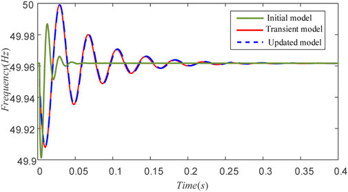
Figure 17. Comparison of frequency response curves between updated model and electromagnetic transient model.

Therefore, the online update strategy proposed in this section enables rapid adaptation of the inverter SFR model to reflect the current system frequency dynamics. It provides accurate support for on-site personnel to assess the real-time frequency stability status, thereby avoiding overly optimistic evaluations caused by outdated models.

5.3.2 Adjustment of control parameters

Under the operating condition corresponding to point 3 in Figure 2, the system exhibits excessively low damping, leading to significant frequency oscillations even under small disturbances.

Once the system damping ratio ${\mathrm{\Gamma }}_{\mathrm{D}}$ is detected to fall below the threshold of 0.2, the model parameter optimization strategy is initiated. Using the online inertia and damping enhancement approach presented in Section 4.2, the system inertia is set to a target value of $J_{\text{opt}}=0.7$ and the damping ratio to ${\mathrm{\Gamma }}_{\text{Dopt}}=0.7$. This setup is used to verify the effectiveness of the optimized parameters in improving the system’s dynamic response and frequency stability.

In this scenario, the parameter adjustment strategy selects $K_{il}$ as the control parameter due to its highest sensitivity. Its original value is 1, and the optimized result gives an updated value of 13. Figure 18 compares the system responses before and after the adjustment under the same step disturbance.

Figure 18

Figure 18. Comparison of frequency response curves between initial model and parameter-adjusted model.

Figure 18 shows that prior to adjusting the control parameter, the system exhibited prolonged frequency oscillations under small disturbances. After the adjustment, the frequency stabilized within 0.06 s. The response time was reduced by 80.1% and the overshoot decreased by 19.8%. By increasing the damping ratio by 0.53 through parameter tuning, system oscillations were effectively suppressed and overall stability was improved.

6 Conclusion

This study investigates the frequency response modeling and application of inverter-based source for off-grid renewable energy systems. The research encompasses model derivation, parameter identification, online model updating, and control parameter adjustment. Based on theoretical analysis and simulation validation, the following conclusions are drawn:

1. A second-order frequency response model of the inverter-based source was developed. Its effectiveness was validated through simulation comparisons with a detailed electromagnetic transient model. The proposed model achieves a desirable balance between accuracy and model order, providing sufficiently accurate representation of the system’s frequency dynamics while significantly reducing the model’s complexity.

2. The dynamic performance indices of the inverter-based frequency response model were derived, and a parameter identification method based on the Levenberg-Marquardt optimization algorithm was proposed. The effectiveness of this method was validated by comparing the system’s observed response with the response of the identified model. All identified parameters closely approached the optimal solution, and the method demonstrated robust convergence even when the initial estimates deviated from the true values.

3. For model application, this study develops two strategies: an online parameter updating mechanism that adapts to shifting operating points, and a parameter adjustment method that enhances system inertia and damping. Simulation results confirm that both approaches accurately update the SFR model and effectively improve damping performance. These capabilities help on-site operators gain reliable insight into real-time frequency stability, avoiding overly optimistic evaluations caused by outdated models. Additionally, the proposed strategy enables prompt enhancement of system damping under severe frequency oscillations, thereby contributing to improved system stability.

The proposed method was validated on a single inverter–single load system. In multi-inverter parallel systems, power sharing and control interactions are expected to have a stronger impact on frequency response. Accordingly, the method needs to be extended to incorporate inverter coupling and network impedance effects. With these refinements, its accuracy and generality in large-scale off-grid renewable energy systems can be further improved.

Data availability statement

Data will be made available on request.

Author contributions

YT: Conceptualization, Methodology, Formal analysis, Investigation, Writing – original draft, Writing – review and editing, Project administration, Funding acquisition. LT: Methodology, Software, Data curation, Writing – original draft, Visualization. YL: Software, Writing – original draft, Visualization. JY: Validation, Supervision, Writing – original draft. KM: Resources, Writing – review and editing.

Funding

The authors declare that financial support was received for the research and/or publication of this article. Project Supported by China Southern Grid Digital Grid Funding (DPGCSG-2024-KF-21).

Conflict of interest

The authors declare that the research was conducted in the absence of any commercial or financial relationships that could be construed as a potential conflict of interest.

The authors declare that this study received funding from China Southern Grid Digital Grid Funding (DPGCSG-2024-KF-21). The funder had the following involvement in the study: the study design, collection, analysis, interpretation of data, the writing of this article, and the decision to submit it for publication.

Generative AI statement

The authors declare that no Generative AI was used in the creation of this manuscript.

Any alternative text (alt text) provided alongside figures in this article has been generated by Frontiers with the support of artificial intelligence and reasonable efforts have been made to ensure accuracy, including review by the authors wherever possible. If you identify any issues, please contact us.

Publisher’s note

All claims expressed in this article are solely those of the authors and do not necessarily represent those of their affiliated organizations, or those of the publisher, the editors and the reviewers. Any product that may be evaluated in this article, or claim that may be made by its manufacturer, is not guaranteed or endorsed by the publisher.

Supplementary material

The Supplementary Material for this article can be found online at: https://www.frontiersin.org/articles/10.3389/fenrg.2025.1676099/full#supplementary-material

References

Abd Elaziz, M., and Oliva, D. (2018). Parameter estimation of solar cells diode models by an improved opposition-based whale optimization algorithm. Energy Convers. Manag. 171, 1843–1859. doi:10.1016/j.enconman.2018.05.062

CrossRef Full Text | Google Scholar

Bai, F., Cui, Y., and Yan, R. (2022). Frequency response of PV inverters toward high renewable penetrated distribution networks. CSEE J. Power Energy Syst. 08 (02), 465–475. doi:10.17775/CSEEJPES.2021.08470

CrossRef Full Text | Google Scholar

Chen, G., Dong, Y., and Liang, Z. (2020). Analysis and reflection on the high quality development of Chinese characteristics new energy in energy transition. Chin. J. Electr. Eng. 40 (17), 5493–5505. doi:10.13334/j.0258-8013.pcsee.200984

CrossRef Full Text | Google Scholar

Gao, B., Yi, L., and Yunhong, L. (2021). Disturbance transmission path and damping characteristics analysis of direct drive wind farm and LCC-HVDC subsynchronous interaction. Chin. J. Electr. Eng. 41 (05), 1713–1729. doi:10.13334/j.0258-8013.pcsee.200187

CrossRef Full Text | Google Scholar

Gao, B., Gang, W., and Shao, B. (2022). Singular perturbation reduction method for direct drive wind farms based on dominance analysis. Chin. J. Electr. Eng. 42 (07), 2449–2462. doi:10.13334/j.0258-8013.pcsee.210492

CrossRef Full Text | Google Scholar

Huang, W., Zhai, S., Lu, X., Liu, Y., Fang, Y., He, W., et al. (2024). Analysis of the impact of voltage control on the frequency response characteristics of grid-forming converter. South. Power Syst. Technol. 18 (5), 102–111. doi:10.13648/j.cnki.issn1674-0629.2024.05.010

CrossRef Full Text | Google Scholar

Junkai, H., Yang, Z., and Yu, J. (2022). Low order modeling method for fast frequency response of wind turbines for frequency stability verification and its error analysis. Chin. J. Electr. Eng. 42 (18), 6752–6766. doi:10.13334/j.0258-8013.pcsee.211559

CrossRef Full Text | Google Scholar

Kang, J., and Xiao, W. (2024). Optimization study on wind and solar capacity ratio of chaidamu desert new energy base in haixi, Qinghai province. Northwest Hydropower (03), 108–113.

Google Scholar

Kouro, S., Leon, J., Vinnikov, D., and Franquelo, L. (2015). Grid-connected photovoltaic systems: an overview of recent research and emerging PV converter technology. IEEE Ind. Electron. Mag. 9 (1), 47–61. doi:10.1109/mie.2014.2376976

CrossRef Full Text | Google Scholar

Liang, J., Qiao, K. J., Yu, K. J., Ge, S., Qu, B., Xu, R., et al. (2020). Parameters estimation of solar photovoltaic models via a self-adaptive ensemble-based differential evolution. Sol. Energy 207, 336–346. doi:10.1016/j.solener.2020.06.100

CrossRef Full Text | Google Scholar

Liu, Q., Heng, Y., Zheng, R., and Chen, S. (2021). “Reduced order modeling of DFIG based on singular perturbation theory,” in IECON 2021 – 47th Annual Conference of the IEEE Industrial Electronics Society. Toronto, ON, Canada: IEEE Industrial Electronics Society. doi:10.1109/IECON48115.2021.9589785

CrossRef Full Text | Google Scholar

Luyang, L., Wang, F., and Chen, L. (2024). Dynamic response modeling and analysis of doubly fed wind turbines to power grid frequency disturbances. Power Syst. Autom. 48 (09), 75–85.

Google Scholar

Ma, M., Ma, Q., and Xiao, C. (2017). Photovoltaic cell parameter estimation using hybrid particle swarm optimization and simulated annealing. Energies 10 (8), 1–14. doi:10.3390/en10081213

CrossRef Full Text | Google Scholar

Qinfeng, M., Su, A., Mingshun, L., Xianqiang, H., Zhu, X., Song, D., et al. (2024). Frequency characteristics of new power system considering the frequency modulation contribution of wind power-photovoltaic-energy storage. South. Power Syst. Technol. 18 (11), 129–140. doi:10.13648/j.cnki.issn1674-0629.2024.11.014

CrossRef Full Text | Google Scholar

Sauer, P. W., and Pai, M. A. (1997). Power system dynamics and stability. Upper Saddle River, NJ: Prentice Hall.

Google Scholar

Wang, M., Guo, J., and Ma, S. (2023). Overview of transient frequency stability analysis and frequency control methods for new energy power systems. Chin. J. Electr. Eng. 43 (05), 1672–1694. doi:10.13334/j.0258-8013.pcsee.221466

CrossRef Full Text | Google Scholar

Xiaokang, H., Wang, Z., Qi, X., Taotao, Q., Lin, H., Cai, C., et al. (2023). Interaction frequency regulation strategy between offshore wind farm and island microgrids considering minimum inertia requirement. South. Power Syst. Technol. 17 (5), 80–90. doi:10.13648/j.cnki.issn1674-0629.2023.05.009

CrossRef Full Text | Google Scholar

Yang, J.-Y., Song, Y. H., and Kook, K. S. (2024). Critical inertia calculation method of generators using energy balance condition in power system. Energies 17, 1097. doi:10.3390/en17051097

CrossRef Full Text | Google Scholar

Yonggang, L., Feng, Y., and Chen, M. (2020). Optimization of control parameters for inverter power generation based on multi time scale reduction. J. North China Electr. Power Univ. Nat. Sci. Ed. 47 (03), 1–9.

Google Scholar

Zhang, J., and Mingjie, L. (2020). Frequency characteristics analysis of high penetration new energy power systems. Chin. J. Electr. Eng. 40 (11), 3498–3507. doi:10.13334/j.0258-8013.pcsee.191265

CrossRef Full Text | Google Scholar

Zhang, J., and Wang, Y. (2021). Integrating physical and data-driven system frequency response modelling for wind-PV-thermal power systems. CSEE J. Power Energy Syst. 4 (7), 137–148. doi:10.1109/TPWRS.2023.3242832

CrossRef Full Text | Google Scholar

Zheng, C., Wang, S., and Zhang, B. (2019). Dynamic frequency characteristics and countermeasures of high penetration power grid with inverter power supply. Grid Technol. 43 (11), 4064–4073.

Google Scholar