Ultra-short-term load forecasting and risk assessment method for distribution networks based on the VMD–DeepAR model

Introduction: With increasing uncertainties on both the generation and load sides in power systems, ultra-short-term load forecasting (USTLF) and risk assessment have become crucial for ensuring the secure and optimal operations of power systems, especially in distribution networks.

Methods: This paper proposed a probabilistic load forecasting method that integrates variational mode decomposition (VMD) with an improved deep autoregressive probabilistic forecasting (DeepAR) model. VMD reduces the non-stationarity of the load sequence, and a future feature enhancement mechanism was introduced to improve the accuracy under multi-step predictions. Based on the proposed method, an integrated assessment framework covering voltage deviations and transformer overload risks was constructed. Exponential aggregation functions and nonlinear normalization methods were utilized to evaluate the combined risk index with multidimensional risk indicators with different units.

Results: Case studies demonstrated that the proposed VMD with the improved DeepAR model improved the accuracy of load forecasting over traditional models.

Discussion: Moreover, the proposed risk assessment method can provide quantitative and systematic early risk-warning support for distribution network operations and decision-making.

1 Introduction

As the requirements of power systems for decarbonization and security become increasingly critical, future power systems will face substantial operational challenges arising from uncertainties on both the generation and demand sides. In particular, electricity consumption behaviors with pronounced temporal variability—such as electric vehicle charging loads and seasonal industrial electricity usage—introduce significant uncertainty into distribution network operating patterns (Deb et al., 2018; Verzijlbergh et al., 2012; Li et al., 2023). Such fluctuations could cause local bus voltages to deviate far from the safe operating range, leading to voltage violations. They can also cause distribution transformers to operate under short-term overload conditions, accelerating equipment insulation aging and even triggering failures, which severely impacts power supply reliability and power quality. To overcome such challenges, accurate load forecasting technologies for short-term and comprehensive risk assessment of distribution networks based on probabilistic methods, which enable the quantitative characterization of risk values, have become key technical foundations for building intelligent distribution network early risk-warning systems.

Ultra-short-term load forecasting (USTLF) plays a critical role in modern distribution networks by providing highly accurate predictions of electricity load over a time horizon of several minutes to a few hours. Its importance is particularly prominent in maintaining the security, stability, and economic efficiency of power system operations. With the increasing integration of distributed energy resources, distribution networks face growing uncertainties and fluctuations. USTLF enables system operators to anticipate rapid load changes, mitigate potential overloads, optimize generation dispatch, and enhance voltage regulation. USTLF methods can be broadly categorized into statistical methods and artificial intelligence (AI) algorithms. Statistical methods include regression models (Momani et al., 2024), exponential smoothing models, and autoregressive integrated moving average models (ARIMAs) (Shaukat et al., 2021). These models have certain advantages in handling trend data but struggle to predict complex, nonlinear load data with time-series. AI algorithms possess powerful nonlinear modeling capabilities and demonstrate strong performance in processing high-dimensional data and capturing complex spatiotemporal dependencies. The typical AI algorithms include long short-term memory (LSTM) networks (Tan et al., 2020; Chen et al., 2025), convolutional neural networks (CNNs) (Farsi et al., 2021), and transformer models. Tan et al. (2020) proposed a hybrid ensemble learning forecasting model based on LSTM networks, introducing a new loss function that integrates peak demand prediction error based on the bias–variance trade-off. An SCKF-LSTM-based trajectory tracking method for electricity–gas integrated energy systems was developed by Chen et al. (2025), demonstrating the effectiveness of combining advanced filtering techniques with deep learning to improve multi-energy system operational accuracy. Farsi et al. (2021) proposed a load forecasting model combining LSTM and CNN. While effective, these models primarily focus on generating single-point forecasts and do not address the need for quantifying predictive uncertainty.

To further enhance the support capability of forecasting information for uncertainty management, load forecasting research has gradually expanded from point forecasting to probabilistic forecasting (Vanting et al., 2021). AI algorithms, represented by deep learning, have also been widely applied in this field. These methods aim to predict the probability distribution of future loads, rather than providing a single-point estimate, thereby offering richer information for system operation and risk assessment (Xu and Chen, 2024; Ryu and Yu, 2024). Typical probabilistic load-forecasting models include the autoregressive recurrent neural network-based deep autoregressive probabilistic forecasting (DeepAR) model (Salinas et al., 2020) and spatiotemporal graph neural networks. Ryu and Yu (2024) proposed a quantile mixture model (Q-mixer) for short-term probabilistic load forecasting. These models excel at extracting features from high-dimensional complex inputs and effectively handling the complex relationships between load and multi-source covariates. Considering that more information with different sources can be captured by various kinds of sensors from future power grids, the capabilities of AI algorithms to integrate future information can be improved (Yang L. et al., 2025).

Ultra-short-term load data exhibit intense fluctuations and typical non-stationary characteristics. To improve the prediction accuracy, signal decomposition methods are widely used in the data preprocessing stage to decompose the complex original sequence into several relatively simple and stationary sub-sequences, providing more predictable inputs for subsequent models. The current signal decomposition methods include empirical mode decomposition (Guo et al., 2019) (EMD) and variational mode decomposition (Cheng et al., 2025) (VMD). Guo et al. (2019) proposed an ensemble empirical mode decomposition (EEMD) method to highlight the local characteristics of original load data and address the mode mixing problem in EMD decomposition. Huang et al. (2021) introduced complete ensemble empirical mode decomposition with adaptive noise (CEEMDAN) into a load forecasting model to better handle the non-stationary nature of load data and reduce mode aliasing. VMD is an adaptive, non-recursive decomposition method that offers a mathematically rigorous alternative to EMD-based techniques. It retains the advantages of EEMD and CEEMDAN, such as noise robustness and resolved mode mixing, while providing greater theoretical solidity (Cheng et al., 2025). These properties make VMD a suitable choice for handling the non-stationary nature of ultra-short-term load data.

Accurate probabilistic load forecasting results will improve the accuracy of system operational risk assessment. The future operational risk of the system can be effectively evaluated and warned based on effective future scenario prediction. Currently, power system risk assessment primarily employs analytical methods or simulation methods (Bie et al., 2024). Analytical methods abstract uncertainty factors such as equipment failure, load fluctuations, and renewable energy output into probability distributions and use probabilistic power flow calculations to assess potential operational risks (Jia et al., 2023). Yang X. et al. (2025) proposed a Gaussian mixture model-based uncertainty modeling approach for power systems incorporating latent variable interactions to enhance the characterization of complex stochastic behaviors. Zhongbo et al. (2025) combined probabilistic power flow with branch power flow to assess the stochastic distribution of voltage fluctuations and energy demand, aiming to optimize coordinated operation for risk reduction. However, these methods require complex formula derivations and rely on simplifying assumptions, such as linearized power flow equations. Thus, it presents limitations when dealing with high-dimensional, nonlinear or strongly coupled scenarios (Villanueva et al., 2014). In contrast, simulation methods use random sampling to replicate system operating states and rely on a large number of repeated numerical experiments to statistically determine the probability distribution of risk indicators, thereby approximating the probabilistic characteristics of the practical systems (Gautam et al., 2021). Although computationally intensive, these methods demonstrate strong applicability and high accuracy in analyzing complex systems (Zhou et al., 2018), making them particularly suitable for the risk assessment of large-scale systems. Zhao and Zhang (2014) incorporated disaster-related factors into power system risk assessment by applying an improved Monte Carlo method to comprehensively evaluate the system risk levels under various possible operating conditions.

Although existing simulation-based risk assessment methods can quantify system operational risk, their results often differ significantly across scenarios, resulting in the absence of a unified benchmark for cross-scenario comparison. To address this limitation, this paper proposes a comprehensive assessment method that integrates ultra-short-term probabilistic load forecasting with standardized aggregation evaluation. Specifically, the DeepAR probabilistic forecasting model is enhanced by incorporating VMD and a future information fusion mechanism. Building on this improvement, a standardized assessment system framework covering voltage violation and transformer overload risks is developed, enabling the effective integration of diverse risk indicators. The main contributions of this paper are listed as follows:

1. An improved DeepAR probabilistic forecasting model, incorporating VMD and future feature fusion, was proposed to more accurately capture the probability distribution of future loads.

2. Quantitative formulations of the voltage violation risk index (VVRI) and the transformer overload risk index (TORI) were developed, along with an exponential aggregation method for risk evaluation.

3. A standardized comprehensive risk index calculation method based on nonlinear transformation and a combined weighting strategy is designed to significantly enhance the comparability of risk assessment results and strengthen decision-support capability.

This paper is organized as follows: Section 2 proposes the improved VMD–DeepAR probabilistic load-forecasting model; Section 3 develops the integrated risk-assessment framework; Section 4 presents case studies validating the model’s performance and risk assessment results; Section 5 is the conclusion of the paper.

2 Ultra-short-term load forecasting

This paper proposes a USTLF approach based on VMD and an improved DeepAR model. By integrating historical data and future known features, the proposed method enables multi-step probabilistic forecasting. The structure of this method is shown in Figure 1.

Figure 1

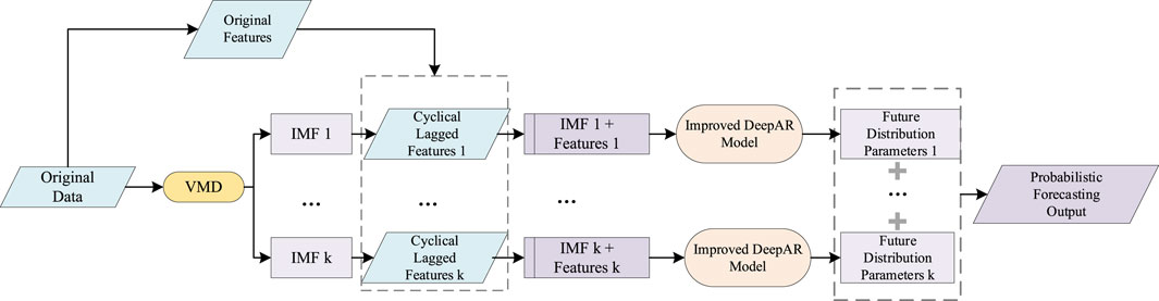
Figure 1. Forecasting model framework.

First, the VMD algorithm decomposes the original load sequence into k intrinsic mode functions (IMFs) with different center frequencies, thereby mitigating the effects of non-stationarity and randomness on the forecasting accuracy. The original load features (such as meteorological and temporal factors) are then combined with each IMF component and its cyclical lagged features to construct an enhanced feature set. The improved DeepAR module subsequently performs probabilistic forecasting for each IMF component independently. Finally, the point forecast and uncertainty quantification of the load are obtained by reconstructing the forecasting results of all IMF components.

2.1 Variational mode decomposition

The VMD is an adaptive, non-recursive signal-processing technique designed for handling non-stationary and nonlinear sequences. Its core principle is to decompose the original signal into several IMFs characterized by sparsity and distinct center frequencies. This process transforms a complex signal into multiple relatively stationary sub-signals with well-defined frequency components, facilitating subsequent analysis and prediction.

VMD performs signal decomposition by formulating and solving a constrained variational optimization problem. The objective of this problem is to minimize the total estimated bandwidth of all modal functions, with the constraint that the sum of all modes equals the original signal. The specific steps are as follows:

First, the unilateral spectrum of each mode is obtained through the Hilbert transform, as shown in Equation 1.

$\left(\delta \left(t\right)+\frac{j}{\pi t}\right)*u_k\left(t\right),(1)$

where u_k(t) represents the kth modal function.

Second, the constrained variational model is constructed, as shown in Equation 2.

$\underset{\left\{u_k\right\}\left\{{\omega }_k\right\}}{\min }\left\{{{\displaystyle \sum _k}‖{\mathrm{\partial }}_t\left[\left(\delta \left(t\right)+\frac{j}{\pi t}\right)*u_k\left(t\right)\right]e^{-j{\omega }_{k}t}‖}_2^2\right\}.(2)$

The constraint is

${\displaystyle \sum _k}{u}_k\left(t\right)=f\left(t\right),(3)$

where f(t) is the original signal and ω_k is the center frequency of each mode.

To address this problem, a quadratic penalty term and Lagrange multipliers are introduced to convert the constrained problem into an unconstrained optimization problem. The alternating direction method of multipliers (ADMM) is then used to iteratively update each modal function and its center frequency, ultimately achieving adaptive signal decomposition. The transformed augmented Lagrangian function is shown in Equation 4.

$\begin{array}{ll}\hfill L\left(\left\{u_k\right\},\left\{{\omega }_k\right\},\lambda \right)& =\alpha {{\displaystyle \sum _k}‖{\mathrm{\partial }}_t\left[\left(\delta \left(t\right)+\frac{j}{\pi t}\right)*u_k\left(t\right)\right]e^{-j{\omega }_{k}t}‖}_2^2\hfill \\ \hfill & +{‖f\left(t\right)-{\displaystyle \sum _k}{u}_k\left(t\right)‖}_2^2+〈\lambda \left(t\right),f\left(t\right)-{\displaystyle \sum _k}{u}_k\left(t\right)〉.\hfill \end{array}(4)$

2.2 Long short-term memory network

The LSTM network is a specialized type of recurrent neural network (RNN) that effectively overcomes the vanishing or exploding gradient problems encountered by traditional RNNs when processing long sequences by introducing gating mechanisms. Its core architecture consists of three gating mechanisms, the forget gate, input gate, and output gate. Through the collaborative operations, the LSTM is able to regulate the selection, retention, and output of historical information. The functions of these gates and the corresponding state update process are described as follows.

1. Forget gate: controls the degree to which the cell state from the previous time step is retained, as shown in Equation 5.

$f_t=\sigma \left(W_f·\left[h_{t-1},x_t\right]+b_f\right).(5)$

2. Input gate: regulates the update of the cell state by current input information, as shown in Equations 6, 7.

$i_t=\sigma \left(W_i·\left[h_{t-1},x_t\right]+b_i\right).(6)$

${\stackrel{\sim }{c}}_t=\tanh \left(W_c·\left[h_{t-1},x_t\right]+b_c\right).(7)$

3. Cell state update: updates the cell state by combining the forget gate and input gate, as shown in Equation 8.

$c_t=f_t*c_{t-1}+i_t*{\stackrel{\sim }{c}}_t.(8)$

4. Output gate: controls the contribution of the current cell state to the output, as shown in Equations 9, 10.

$o_t=\sigma \left(W_o·\left[h_{t-1},x_t\right]+b_o\right).(9)$

$h_t=o_t*\tanh \left(c_t\right).(10)$

In the above formulas, W_f, W_i, W_c, and W_o are the weight matrices for the forget gate, input gate, cell state, and output gate, respectively; b_f, b_i, b_c, and b_o are the bias vectors for the forget gate, input gate, cell state, and output gate, respectively.

2.3 DeepAR probabilistic forecasting module and its improvement

DeepAR is a probabilistic forecasting method based on autoregressive RNNs proposed by Salinas et al. (2020). It is suitable for joint modeling and forecasting of large numbers of related time-series. Its core concept is to employ a global model that learns the shared characteristics across all time-series and produces probability distributions of future values, rather than single-point forecasts, thereby explicitly quantifying uncertainty.

DeepAR uses RNNs as the basic network structure to model time-series in an autoregressive fashion. The model seeks to learn the conditional probability distribution of future values, decomposing the joint distribution into a product of likelihood factors, as shown in Equation 11.

$P\left(z_{i,t_0:T}\left|z_{i,1:t_0-1},x_{i,1:T}\right.\right)={\displaystyle \prod _{t=t_0}^T}p\left(z_{i,t}\left|\theta \left(h_{i,t}\right)\right.\right),(11)$

where z_i,t is the value of the ith time-series at time t, t₀ is the forecast start time, x_i,t are the known covariates, and θ(h_i,t) are the distribution parameters mapped from the LSTM hidden state h_i,t.

For continuous load data, it is typically assumed to follow a Gaussian distribution. The distribution parameters are calculated as shown in Equations 12, 13.

$\mu \left(h_{i,t}\right)=w_{\mu }^{\top }{h}_{i,t}+b_{\mu },(12)$

$\sigma \left(h_{i,t}\right)=\log \left(1+\exp \left(w_{\sigma }^{\top }{h}_{i,t}+b_{\sigma }\right)\right),(13)$

where μ is the mean of the Gaussian distribution, σ is the standard deviation of the Gaussian distribution, w_μ and w_σ are the weight vectors for calculating the mean and standard deviation, respectively, and b_μ and b_σ are the bias terms for calculating the mean and standard deviation, respectively.

The original DeepAR model only uses historical sequences and covariates up to the current time for prediction and does not explicitly utilize future known features, such as future dates and holidays. This paper proposes an improved DeepAR structure that introduces a future feature fusion mechanism between the LSTM encoder and the probability distribution layer, as shown in Figure 2.

Figure 2

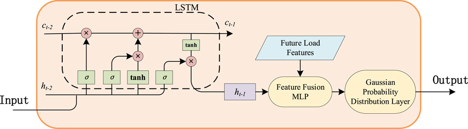
Figure 2. Improved DeepAR module.

1. Future feature projection: the known features for the future Mtime steps are flattened and projected through a fully connected layer, as shown in Equation 14:

$F_i=\text{ReLU}\left(W_F·\text{flatten}\left(x_{i,t_0:t_0+M-1}\right)+b_F\right),(14)$

where F_i is the feature vector obtained after projecting the future features, W_F is the weight matrix for the future features, and b_F is the bias vector for the future features.

2. Feature fusion: the hidden state output from the last layer of the LSTM is concatenated with the future feature projection vector, and a multilayer perceptron (MLP) is used to further fuse the feature information, as shown in Equation 15.

$h_{mlp}=MLP\left(\left[h_{i,t_0-1};F_i\right]\right).(15)$

The output of the MLP, h_mlp, replaces the hidden state h_i,t used for parameter estimation in the original DeepAR, ultimately obtaining the load probability distribution parameters for the future M time steps. Unlike the original DeepAR model that generates forecasts autoregressively (step-by-step), our improved module directly outputs the parameters of the probability distributions for all future M time steps in a single forward pass. This is achieved through separate linear output layers that map h_mlp to vectors of the means and standard deviations for the entire forecast horizon. This non-autoregressive design is enabled by the fact that all future known features (e.g., calendar information) are already available at the time of forecasting. By processing the entire future context F_i simultaneously, the model can learn interdependencies between different future time steps and generate a coherent multi-step forecast without the risk of error propagation inherent in autoregressive models. This structure enables the model to simultaneously utilize the temporal dependencies of historical sequences and the prior knowledge of future known information, making full use of the available information for load forecasting, thereby improving the accuracy and reliability of load forecasts.

3 Integrated risk assessment methods

To achieve a comprehensive assessment of future distribution network operations, this paper develops an integrated risk assessment framework. This framework focuses on the distribution network voltage violation risk and transformer overload risk as the primary targets. They represent two of the most prevalent and critical operational challenges in distribution system management. The specific process is shown in Figure 3.

Figure 3

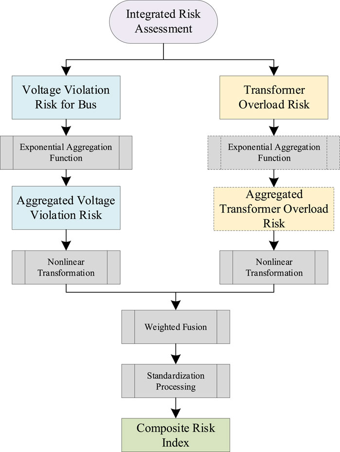
Figure 3. Risk assessment framework.

First, the voltage violation risk for each bus is assessed independently, obtaining the voltage deviation risk indicator for each bus. Subsequently, an exponential aggregation function is used to synthesize the risks of all buses, forming a system-level voltage violation risk indicator. Simultaneously, the overload risk of distribution transformers is assessed. If multiple transformers exist, an exponential aggregation function is similarly used to synthesize the overload risk indicators of all transformers, obtaining a system-level transformer overload risk indicator. Furthermore, a nonlinear transformation and weighted fusion method is utilized to combine the above two types of system risk indicators, resulting in a comprehensive risk indicator for each time step. Finally, risk indicator output standardization is performed by setting extreme risk thresholds.

When assessing the operational risk of a power system at a specific time, it is necessary to comprehensively consider the probability of risk events occurring and the severity of their consequences, thereby constructing a quantitative risk indicator that integrates probability and severity (Li et al., 2015). This paper utilizes a risk-seeking utility function (Diedrich, 2024) to quantify the severity of bus voltage violations and transformer overloads, respectively. The risk indicator value is defined as the product of severity and occurrence probability.

3.1 Voltage violation risk index

When the per-unit voltage value V_i,s at bus i under system state s exceeds the normal operating range [V_min, V_max], the bus is considered to be in a voltage violation state. Quantifying the value by which the bus voltage exceeds the system’s normal operating upper or lower limit allows for the assessment of the severity of the voltage violation. Furthermore, by integrating the voltage violation probability and severity, the VVRI for the bus (VVRI(B)) is obtained, as shown in Equations 16, 17:

$S_{V,i,s}=\frac{e^{\max \left(V_{i,s}-V_{\max },V_{\min }-V_{i,s},0\right)}-1}{e-1},(16)$

$R_{VVRI\left(B\right),i}={\displaystyle \sum _s}{p}_s·S_{V,i,s},(17)$

where V_i,s represents the per-unit voltage value at bus i under scenario s, S_V,i,s represents the severity of the voltage violation at bus i under scenario s, p_s represents the occurrence probability of scenario s, and R_VVRI(B),i represents the voltage violation risk indicator for bus i.

To capture the “high-risk dominance” characteristic within the system, an exponential aggregation function is used to synthesize the voltage violation risk indicators of all buses, obtaining the system-level VVRI, as shown in Equation 18:

$R_{VVRI}=\frac{1}{\alpha }\ln \left(\frac{1}{N}{\displaystyle \sum _{i=1}^N}\exp \left(\alpha ·R_{VVRI\left(B\right),i}\right)\right),(18)$

where N is the number of aggregated indicators, R_VVRI is the voltage violation risk value, and α is the aggregation factor. The value of α is recommended to be in the range of 500–2,000. The influence of different α values on the aggregated indicator will be discussed in Section 4.2.2.

3.2 Transformer overload risk index

The load rate of a distribution transformer during normal operation is typically below 80%. However, under extreme scenarios with intense load fluctuations (such as industrial impact loads), the transformer may operate under heavy load or even overload conditions. Although transformers possess a certain overload operation capability, continuous or frequent overload operation will lead to significant internal temperature rise, causing equipment overheating, accelerating the thermal aging of insulation materials, and reducing their mechanical strength and electrical performance. This substantially shortens equipment lifespan and poses a serious threat to the power supply reliability and operational safety of the distribution system. Based on this, this paper integrates the transformer overload degree and the probability of overload scenarios to define the TORI, as shown in Equations 19, 20:

$S_{T,j,s}=\frac{e^{\max \left(L_{j,s}-L_{j,\max },0\right)}-1}{e-1},(19)$

$R_{TORI,j}={\displaystyle \sum _s}{p}_s·S_{T,j,s},(20)$

where L _j,s is the load rate of transformer j under scenario s, L_{j, max} is the maximum normal operating load rate for transformer j, taken as 100% in this paper, S_{T, j,s} is the overload degree of transformer j under scenario s, and R_TORI,j is the overload risk indicator for transformer j.

For cases involving multiple transformers, an exponential aggregation method is used to aggregate the overload risk indicators, as shown in Equation 21:

$R_{TORI}=\frac{1}{\alpha }\ln \left(\frac{1}{N}{\displaystyle \sum _{j=1}^N}\exp \left(\alpha ·R_{TORI,j}\right)\right).(21)$

3.3 Comprehensive risk index

To accurately quantify the system risk, this paper integrates the above two risk indicator values of different magnitudes (R_VVRI and R_TORI) into a standardized comprehensive risk index (CRI) within the range [0, 1], as shown in Equation 22.

$R_{CRI}=\max \left(0,\min \left(1,\beta ·\left[w_V·\tanh \left({R_{VVRI}}^{1/p}\right)+w_T·\tanh \left({R_{TORI}}^{1/q}\right)\right]\right)\right).(22)$

First, a power function and a tanh function are applied to the VVRI and TORI indicator values for nonlinear transformation. The power operation is used to adjust the sensitivity of the indicators; by setting risk sensitivity coefficients (p, q) greater than 1, the influence of smaller risk values is amplified, making the model more sensitive to low-risk values. Subsequently, the tanh operation is applied to the power-transformed results to prevent any single extreme value from having an excessive impact on the final result.

Second, the nonlinearly transformed indicator values are weighted and summed. Weights are set to reflect the relative importance of each risk in the comprehensive indicator. Here, w_V is the weight for the VVRI indicator, and w_T is the weight for the TORI indicator.

Finally, a scaling factor β indicates the extreme risk threshold, and the weighted sum is standardized using max and min logic. When there is no system risk during the period, the CRI outputs 0. When the system risk exceeds the extreme risk threshold, the CRI outputs 1. When the system risk is below the extreme risk threshold but not zero, the actual risk value is output.

Unlike direct linear weighting methods, the proposed comprehensive method effectively fuses risk indicators of different natures and units into a unified, standardized indicator value. Conventional linear methods often lack clear physical boundaries and cannot adapt to different risk tolerance scenarios. In contrast, the proposed approach produces an output with well-defined physical meaning and bounds, offering both interpretability and adjustable sensitivity. This enhances system-level risk perception and supports operational decision-making across diverse contexts.

The risk quantification and integration methods presented are not limited to the two risks discussed above. Instead, they provide a generalizable framework that can be extended to assess other operational risks in distribution networks, such as line overloads or power factor deterioration.

4 Case study

4.1 Forecasting model implementation and performance validation

To verify the reliability of the proposed model, load data from a region in Southwest China for the year 2024 are selected for case analysis. The time span of the load data is from 1 February 2024 to 31 December 2024, with a sampling interval of 15 min, totaling 32,160 samples. Seven feature values are extracted (including three cyclical lagged features and four time features), as shown in Table 1.

Table 1

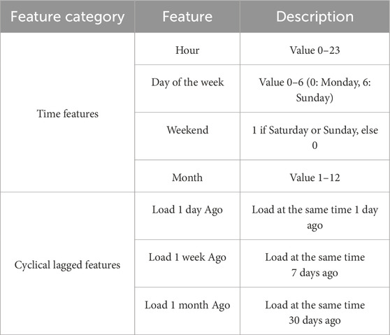
Table 1. Feature variables.

4.1.1 Model settings

The VMD decomposition is performed by numerically solving the constrained variational problem defined in Equations 2–4, with the penalty parameter α in Equation 4 set to 1,000 and the ADMM convergence tolerance set to 1e-7. To balance prediction efficiency and accuracy, the number of decomposition modes is set to 4. A segment of 5,000 sampling points is selected to display the VMD decomposition results. The original load curve and the sequences decomposed using the VMD method are shown in Figure 4. The figure shows that the decomposed sequences exhibit clear periodicity and stable frequency, without mode mixing.

Figure 4

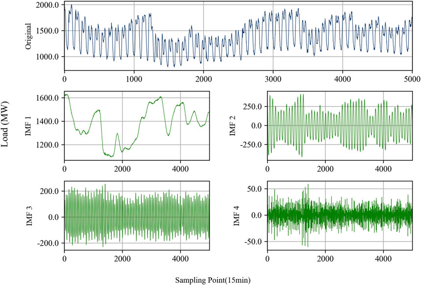
Figure 4. VMD decomposition results of load data.

Historical data from the previous 8 h (32 time steps) are used to predict the power load for the next 4 h (16 time steps). In the improved DeepAR forecasting module, the LSTM module has two layers, with the number of neurons per layer set to 128. After fusing historical data and future features, a 2-layer MLP is set up with 256 and 128 neurons, respectively. The dropout rate for each layer is set to 0.2. The total dataset is divided into training, validation, and test sets in a 7:1:2 ratio. The negative log-likelihood (NLL) loss function is used, with a batch size of 128 and a learning rate of 0.001. The number of iterations is not limited, and an early stopping strategy (stopping training when model performance on the validation dataset degrades) is adopted to ensure the model’s generalization ability.

4.1.2 Point forecasting result comparison

The mean value of the model output is used as the point forecast of the load. The mean absolute error (MAE), root mean square error (RMSE), mean absolute percentage error (MAPE), and the coefficient of determination (R²) are selected as evaluation metrics. To validate the effectiveness of the proposed model, its forecasting results are compared with those of typical forecasting models (BPNN, GRU, LSTM, and VMD–LSTM) and the original DeepAR and VMD–DeepAR models. These typical models are configured with two hidden layers and 128 neurons per layer. They are followed by two fully connected layers with 256 and 128 neurons, respectively, and use the Huber loss function. Other settings are consistent with the proposed model. The point forecast evaluation results are shown in Table 2.

Table 2

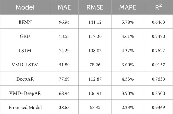
Table 2. Point forecasting evaluation results of different models.

As shown in Table 2, the improved model proposed in this paper outperforms the typical forecasting models across all four metrics. Compared to the VMD–LSTM model, the MAE, RMSE, and MAPE metrics of the proposed model decreased by 25.39%, 13.98%, and 25.67%, respectively. Compared to the original VMD–DeepAR model, the MAE, RMSE, and MAPE metrics of the proposed model decreased by 43.94%, 37.05%, and 42.82%, respectively. This demonstrates the accuracy and superior performance of the improved model in load forecasting.

4.2 Risk scenario generation and comprehensive assessment results

The IEEE 13-bus distribution network system from Aref et al. (2012) is used for case analysis, with several simplifications applied. The transformer at bus 6 is removed, and bus 1 is retained as a pure power source connection without local load. These modifications simulate a low-voltage distribution station area scenario supplied by a single transformer.

Load data from a specific 12-bus low-voltage distribution network in Southwest China are used as the load input for buses 2–13 in the above system. The typical daily load curves for each bus are shown in Figure 5. The figure shows that the selected loads include the impact loads and low-fluctuation loads.

Figure 5

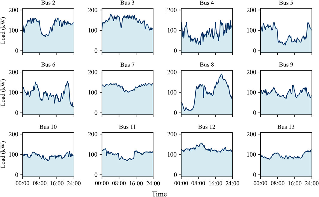
Figure 5. Typical daily load curves for each bus.

4.2.1 Load scenario construction

Based on the proposed improved VMD–DeepAR probabilistic load forecasting model, USTLF is performed for the loads at each of the above buses. Specifically, historical data from the previous 8 h are used to predict the power load for the next 4 h. The data period is from 1 February 2024 to 31 December 2024, with a sampling interval of 15 min, totaling 32,160 samples. Seven load-influencing factors are selected as features, and other settings for the load forecasting model are the same as in Section 4.1.

VMD decomposition is applied to each load. Given the differences in the dynamic characteristics of each bus load, the number of VMD decomposition modes k is determined based on their historical trend characteristics. Taking bus 9 as an example, a segment of 5,000 sampling points is selected to display its VMD decomposition results. The original load curve and the sequences decomposed using the VMD method are shown in Figure 6. The figure shows that IMF1 primarily describes the overall load variation trend within a monthly cycle, IMF2 mainly describes the daily cyclical variation characteristics of the load, and the remaining modes describe the intra-day fluctuation characteristics of the load.

Figure 6

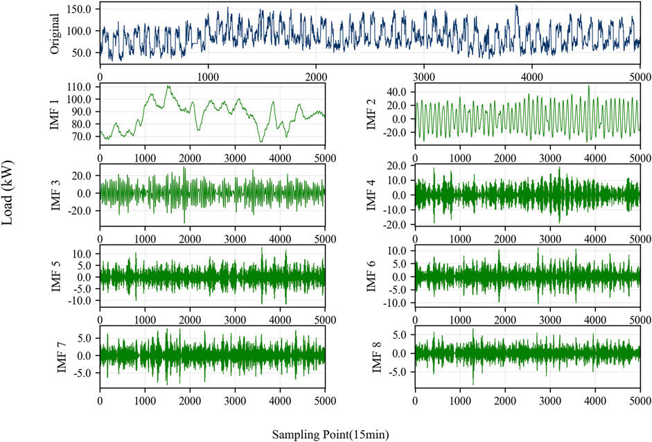
Figure 6. VMD decomposition results of bus 9 load data.

The forecasting accuracy evaluation results for each bus load are shown in Table 3. The table shows that 50% of the bus load forecasts achieve accuracy above 95%, demonstrating the prediction accuracy and reliability of the proposed model.

Table 3

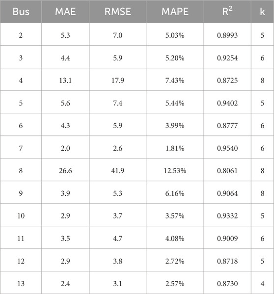
Table 3. Load forecasting accuracy evaluation results.

Based on the mean and standard deviation of the load forecast output by the probabilistic forecasting model, a Gaussian distribution model for the future load is constructed. For a selected typical day, a Monte Carlo simulation with 5,000 samples is performed. This simulation generates load data for 96 time-points under various scenarios, which is then used for risk assessment.

4.2.2 Integrated risk assessment results

Based on the multi-scenario load sampling data generated by Monte Carlo simulation, the integrated risk assessment model constructed in Section 3 is applied. This model conducts a refined, time-series evaluation of the distribution network’s risk level under different operating states. The lower limit of the per-unit bus voltage under normal conditions is defined as 0.95 p.u., and the upper limit is defined as 1.05 p.u. A transformer bank with a total rated capacity of 1,600 kVA (rated active power output of 1,552 kW) is connected at bus 1, and the maximum load rate (L_{j, max}) for the transformer is set to 100%.

According to Formulas 16, 17, the curves of the VVRI(B) for each bus over time are obtained, as shown in Figure 7. To evaluate the impact of the aggregation factor α on the aggregated voltage violation risk indicator in Formula 18, the VVRI is computed and compared for different values of α (500, 1,000, and 2,000), as shown in Figure 8.

Figure 7

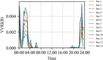
Figure 7. VVRI(B) variation curve over time.

Figure 8

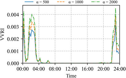
Figure 8. VVRI variation curves over time for different values of α

The figures show that periods of voltage violation risk mainly occur between 18:00 and 08:00 the next day. The risk curve exhibits multiple steep peaks, which is highly consistent with the load fluctuation pattern. Based on the daily load curve (Figure 5) and further analysis of load characteristics, it can be inferred that the impact industrial loads at buses 2, 4, and 6 reach peak usage simultaneously during the night. This concurrent peak demand causes intense local voltage fluctuations. Furthermore, as this system is a radial network supplied by a single source, the voltage quality gradually decays along the supply radius. Buses 9 and 10, located at the end of the supply line, exhibit the longest electrical distance and significant impedance accumulation effects. These factors result in larger voltage drops, making these buses sensitive areas for voltage violations. Consequently, their risk values are significantly higher than those of buses closer to the power source.

Based on Figure 8, the VVRI curves show consistent trends under different aggregation factors α, but their values differ. Specifically, as α increases, the VVRI value approaches the maximum VVRI(B) value among all the buses. This means it better reflects the “high-risk dominance” feature in the system’s voltage violation risk. As a result, it more effectively captures weak operational points in the system. To ensure that the VVRI value accurately represents the inherent uneven distribution of risks in practical operation, the aggregation factor α is set to 1,000 for subsequent risk analysis.

According to Formulas 19, 20, the variation curve of the TORI value at each time-point is obtained, as shown in Figure 9. The TORI indicator shows that the overload risk mainly occurs during the 01:30–03:00 period, with significant risk peaks also appearing at 00:15 and 23:00. This distribution pattern results from multiple bus loads simultaneously reaching their peaks during the night. Such concurrent peak demand causes the transformer’s short-term load rate to rise sharply and significantly increases the probability of overload. The constructed TORI indicator integrates both overload severity and its occurrence probability. It accurately reflects the operational risk of the transformer under extreme load fluctuations, demonstrating strong early warning capability and clear physical interpretability.

Figure 9

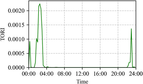
Figure 9. TORI variation curve over time.

To analyze the specific influence of the scaling factor β on CRI in Formula 22, the values of β are set to 5, 8, and 10, with risk sensitivity coefficients fixed at p = 4 and q = 3 and weights for each indicator set to 0.5. The resulting CRI curves under different β values are shown in Figure 10.

Figure 10

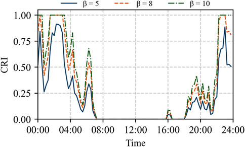
Figure 10. CRI variation curves over time for different values of β

As shown in Figure 10, the CRI effectively integrates both the VVRI and TORI, successfully capturing the system’s low-risk periods between 04:00–08:00 and 18:00–20:00. These intervals exhibit low values of both VVRI and TORI (below 0.0002), which are not easily distinguishable in Figures 8, 9 but are clearly reflected in the dynamic variation of the CRI in Figure 10. Moreover, the sensitivity of the system to risk increases with higher values of β. Specific examples include the following scenarios:

1. When β = 5, the CRI remains below 1 throughout the day, indicating that extreme risk levels are never reached.

2. When β = 8, the CRI reaches 1 during 01:30–03:00 and 22:30–23:00, exceeding the extreme risk threshold. The low-risk periods show higher CRI values (approximately 0.3), with more pronounced variations.

3. When β = 10, the period from 23:00 to 24:00 is also identified as extreme risk.

In summary, the value of β can be adjusted according to the system’s operational risk tolerance in different scenarios to reflect appropriate risk levels. Similarly, the weight allocation in Equation 22 can be further adjusted based on specific system operational priorities, which would proportionally influence the contribution of each risk indicator to the comprehensive risk index. Furthermore, since (22) integrates risk indices of different magnitudes (VVRI and TORI) into a standardized comprehensive risk indicator bounded within [0, 1], it provides clear physical interpretation and comparable risk levels across various operational scenarios.

Based on the case analysis results presented above, the proposed comprehensive risk assessment indicator system demonstrates the following significant advantages:

1. The modeling approach that integrates probability and severity ensures that the risk quantification results contain both the likelihood of events and the severity of consequences, making them more meaningful for practical applications.

2. The introduced aggregation factor α and scaling factor β allow the system to be flexibly adapted to different operational scenarios and risk tolerance requirements. By adjusting α, the dominance of high-risk components can be enhanced or reduced, while modifying β alters the system’s sensitivity to risk threshold violation.

3. The exponential aggregation function enhances the dominant effect of high-risk components within the distribution network, aligning with the short-board management of practical needs in power systems.

4. Through nonlinear transformation and standardization, the CRI indicator integrates risks of different natures and units, offering clearly defined physical boundaries and intuitive interpretability. This capability supports operators in holistic risk assessment and provides a reliable basis for adjusting operational strategies and formulating risk prevention and control measures.

5 Conclusion

This paper focuses on developing USTLF and integrated risk assessment methods for distribution networks. A probabilistic forecasting approach that combines VMD with an improved DeepAR model was proposed, along with a systematic integrated risk-assessment framework. Empirical analysis through case studies validates the effectiveness and practicality of the proposed methods.

The DeepAR model was improved by introducing a future feature fusion mechanism. By concatenating and fusing future known features with the hidden state of historical sequences, the accuracy of the model in multi-step probabilistic load forecasting was significantly improved. The results of case studies indicate that the improved model outperforms comparison models on metrics such as MAE, RMSE, and MAPE, verifying the important role of future feature information in enhancing forecasting performance.

A hierarchically aggregated risk-assessment framework was developed. Based on risk severity and occurrence probability, quantitative formulations for the VVRI and TORI were developed, along with an exponential index aggregation method. Furthermore, a nonlinear transformation and weighted fusion approach was applied to combine VVRI and TORI into a unified standardized CRI. Case analysis shows that this framework can effectively integrate risks of different natures, accurately identify the system’s weak links and high-risk periods, and provide a clear and quantitative basis for operational decision-making.

In summary, the improved VMD–DeepAR model and risk assessment framework proposed in this paper not only enhances the accuracy and robustness of load forecasting but also provides an effective tool for the refined and systematic evaluation of operational risks in distribution networks. Future work could integrate the risk assessment method with distribution network structure optimization, dynamically adjusting network operation modes during predicted high-risk periods to enhance system resilience against extreme events.

Data availability statement

The original contributions presented in the study are included in the article/supplementary material; further inquiries can be directed to the corresponding author.

Author contributions

TX: Conceptualization, Writing – original draft. HL: Writing – original draft, Formal Analysis. TF: Writing – original draft, Investigation. LH: Writing – review and editing, Methodology. QW: Writing – review and editing, Data curation. SW: Writing – review and editing, Investigation.

Funding

The author(s) declare that financial support was received for the research and/or publication of this article. This research was funded by the science and technology program of Guizhou Power Grid Corporation, grant number 060000KC23110059, and the APC was funded by the same funding.

Conflict of interest

Authors TX, HL, TF, and LH were employed by the China Southern Power Grid Guizhou Power Supply Co., Ltd.

Authors QW and SW were employed by Dongfang Electronics Co., Ltd.

Generative AI statement

The author(s) declare that no Generative AI was used in the creation of this manuscript.

Any alternative text (alt text) provided alongside figures in this article has been generated by Frontiers with the support of artificial intelligence and reasonable efforts have been made to ensure accuracy, including review by the authors wherever possible. If you identify any issues, please contact us.

Publisher’s note

All claims expressed in this article are solely those of the authors and do not necessarily represent those of their affiliated organizations, or those of the publisher, the editors and the reviewers. Any product that may be evaluated in this article, or claim that may be made by its manufacturer, is not guaranteed or endorsed by the publisher.

References

Aref, A., Davoudi, M., Razavi, F., and Davoodi, M. (2012). Optimal DG placement in distribution networks using intelligent systems. Energy Power Eng. 4 (2), 92–98. doi:10.4236/epe.2012.42013

CrossRef Full Text | Google Scholar

Bie, Z., Bian, Y., Zhang, L., Huang, Y., and Li, G. (2024). Key technologies of risk prevention and emergency management against extreme events for new power systems. Proc. CSEE 44 (18), 7049–7068. doi:10.13334/j.0258-8013.pcsee.241046

CrossRef Full Text | Google Scholar

Chen, L., Li, Y., Cai, J., Gu, S., and Yan, Y. (2025). SCKF-LSTM-based trajectory tracking for electricity-gas integrated energy system. IEEE Trans. Industrial Inf. 21 (6), 4296–4305. doi:10.1109/tii.2024.3523544

CrossRef Full Text | Google Scholar

Cheng, Q., Shi, J., and Cheng, S. W. (2025). Short-term load forecasting based on similar day theory and BWO-VMD. Energies 18 (9), 2358. doi:10.3390/en18092358

CrossRef Full Text | Google Scholar

Deb, S., Tammi, K., Kalita, K., and Mahanta, P. (2018). Impact of electric vehicle charging station load on distribution network. Energies 11 (1), 178. doi:10.3390/en11010178

CrossRef Full Text | Google Scholar

Diedrich, R. (2024). Combining Savage and Laplace: a new approach to ambiguity. Theory Decis. 97 (3), 423–453. doi:10.1007/s11238-024-09980-0

CrossRef Full Text | Google Scholar

Farsi, B., Amayri, M., Bouguila, N., and Eicker, U. (2021). On short-term load forecasting using machine learning techniques and a novel parallel deep LSTM-CNN approach. IEEE Access 9, 31191–31212. doi:10.1109/access.2021.3060290

CrossRef Full Text | Google Scholar

Gautam, P., Piya, P., and Karki, R. (2021). Resilience assessment of distribution systems integrated with distributed energy resources. IEEE Trans. Sustain. Energy 12 (1), 338–348. doi:10.1109/tste.2020.2994174

CrossRef Full Text | Google Scholar

Guo, W., Jiang, X., Luo, Y., and Han, Q. (2019). Short-term load forecasting in a certain area based on EEMD-GABP. Electr. Power Eng. Technol. 38 (6), 93–98.

Google Scholar

Huang, J., Zhou, Z., Li, C., Liao, Z., and Liu, P. X. (2021). A decomposition-based multi-time dimension long short-term memory model for short-term electric load forecasting. IET Generation, Transm. Distribution 15 (24), 3459–3473. doi:10.1049/gtd2.12265

CrossRef Full Text | Google Scholar

Jia, M., Cao, Q., Shen, C., and Hug, G. (2023). Frequency-control-aware probabilistic load flow: an analytical method. IEEE Trans. Power Syst. 38 (6), 5170–5187. doi:10.1109/tpwrs.2022.3223884

CrossRef Full Text | Google Scholar

Li, X., Zhang, X., Wu, L., Lu, P., and Zhang, S. (2015). Transmission line overload risk assessment for power systems with wind and load-power generation correlation. IEEE Trans. Smart Grid 6 (3), 1233–1242. doi:10.1109/tsg.2014.2387281

CrossRef Full Text | Google Scholar

Li, Y., Zhang, S., Li, Y., Cao, J., and Jia, S. (2023). PMU measurements-based short-term voltage stability assessment of power systems via deep transfer learning. IEEE Trans. Instrum. Meas. 72, 1–11. doi:10.1109/tim.2023.3311065

PubMed Abstract | CrossRef Full Text | Google Scholar

Momani, M. A., Tashtush, S. A., Shahrour, R. J., and Alsatari, A. M. (2024). Modeling of long-term load forecast in Jordan based on statistical techniques. J. Electr. Comput. Eng. 2024, 8255513. doi:10.1155/2024/8255513

CrossRef Full Text | Google Scholar

Ryu, S., and Yu, Y. (2024). Quantile-mixer: a novel deep learning approach for probabilistic short-term load forecasting. IEEE Trans. Smart Grid 15 (2), 2237–2250. doi:10.1109/tsg.2023.3290180

CrossRef Full Text | Google Scholar

Salinas, D., Flunkert, V., Gasthaus, J., and Januschowski, T. (2020). DeepAR: probabilistic forecasting with autoregressive recurrent networks. Int. J. Forecast. 36 (3), 1181–1191. doi:10.1016/j.ijforecast.2019.07.001

CrossRef Full Text | Google Scholar

Shaukat, M. A., Shaukat, H. R., Qadir, Z., Munawar, H. S., and Mahmud, M. A. P. (2021). Cluster analysis and model comparison using smart meter data. Sensors 21 (9), 3157. doi:10.3390/s21093157

PubMed Abstract | CrossRef Full Text | Google Scholar

Tan, M., Yuan, S., Li, S., Su, Y., and He, F. (2020). Ultra-short-term industrial power demand forecasting using LSTM based hybrid ensemble learning. IEEE Trans. Power Syst. 35 (4), 2937–2948. doi:10.1109/tpwrs.2019.2963109

CrossRef Full Text | Google Scholar

Vanting, N. B., Ma, Z., and Jørgensen, B. N. (2021). A scoping review of deep neural networks for electric load forecasting. Energy Inf. 4, 49. doi:10.1186/s42162-021-00148-6

CrossRef Full Text | Google Scholar

Verzijlbergh, R. A., Grond, M. O. W., Lukszo, Z., Slootweg, J. G., and Ilic, M. D. (2012). Network impacts and cost savings of controlled EV charging. IEEE Trans. Smart Grid 3 (3), 1203–1212. doi:10.1109/tsg.2012.2190307

CrossRef Full Text | Google Scholar

Villanueva, D., Feijóo, A. E., and Pazos, J. L. (2014). An analytical method to solve the probabilistic load flow considering load demand correlation using the DC load flow. Electr. Power Syst. Res. 110, 1–8. doi:10.1016/j.epsr.2014.01.003

CrossRef Full Text | Google Scholar

Xu, C., and Chen, G. (2024). Interpretable transformer-based model for probabilistic short-term forecasting of residential net load. Int. J. Electr. Power Energy Syst. 155, 109515. doi:10.1016/j.ijepes.2023.109515

CrossRef Full Text | Google Scholar

Yang, L., Duan, Q., Pan, B., and Wang, Z. (2025a). Post-pandemic holiday load forecasting considering social factors influences based on TL-Informer-LightGBM model. Electr. Power Syst. Res. 247, 111861. doi:10.1016/j.epsr.2025.111861

CrossRef Full Text | Google Scholar

Yang, X., Li, Y., Zhao, Y., Li, Y., and Wang, Y. W. (2025b). Gaussian mixture model uncertainty modeling for power systems considering mutual assistance of latent variables. IEEE Trans. Sustain. Energy 16 (2), 1483–1486. doi:10.1109/tste.2024.3356259

CrossRef Full Text | Google Scholar

Zhao, X. L., and Zhang, J. H. (2014). Power system risk assessment software design under impact of disaster conditions. Appl. Mech. Mater. 441, 204–207. doi:10.4028/www.scientific.net/amm.441.204

CrossRef Full Text | Google Scholar

Zhongbo, C., Liang, L., and Chao, L. (2025). Optimized coordination of electric vehicles, distributed compensation devices, and distributed generation for risk mitigation in radial distribution networks. IET Renew. Power Gener. 19 (1), e70019. doi:10.1049/rpg2.70019

CrossRef Full Text | Google Scholar

Zhou, G., Bo, R., Chien, L., Zhang, X., and Su, D. (2018). GPU-accelerated algorithm for online probabilistic power flow. IEEE Trans. Power Syst. 33 (1), 1132–1135. doi:10.1109/tpwrs.2017.2756339

CrossRef Full Text | Google Scholar