An optimization planning method for rural distribution systems considering on-load tap changers and energy storage

Under the guidance of the “dual carbon” target, rural distribution systems are increasingly affected by power fluctuations and voltage violations owing to the growing penetration of distributed photovoltaic (PV) generation. To address these issues, we propose an optimization planning method for rural distribution systems by considering on-load tap changers (OLTCs), energy storage systems (ESSs), and auxiliary flexible interconnection devices such as soft open points (SOPs). Accordingly, we developed a two-level optimization model: the upper level minimizes the total planning and operational costs by determining the optimal deployment of OLTCs and ESSs under technical and economic constraints; the lower level evaluates the system reliability by calculating the expected energy not supplied (EENS) based on the fault impact matrix (FIM) while ensuring network connectivity and exclusive transfer paths. We also propose an iterative strategy to solve the two-level optimization model, where the planning decisions of the upper level and reliability evaluation solutions of the lower level interact until the convergence condition is satisfied. The framework of the iterative strategy was implemented in the AMPL modeling tool along with the Gurobi solver to ensure computational efficiency. The simulation results indicate that the proposed method achieves 100% PV accommodation, reduces the EENS by over 50%, and reduces the power system costs by approximately 16%, thereby improving both the economic performance and reliability effectively.

1 Introduction

Under the “dual carbon” strategy, the increasing penetration of distributed photovoltaic (PV) generation in rural areas has become a key challenge that restricts low-carbon transition of the distribution networks (Schum and Lin, 2012). The inherent randomness and volatility of PV generation significantly intensify the fluctuations in the net load. Moreover, the traditional radial network structures expose other limitations such as insufficient supply margins, reverse power flow, and voltage violations under multisource operation scenarios (Lin et al., 2023). To address these issues, flexible interconnection technologies based on intelligent soft open points (SOPs) have been demonstrated to offer notable advantages via reconfiguring the network topology through multiterminal power transfer, thereby improving the power balance between supply areas and enhancing the integration of renewable energy (Ji et al., 2019). However, relying solely on SOPs cannot fully mitigate the renewable energy fluctuations; hence, energy storage systems (ESSs) with fast responses and energy-shifting capabilities have become essential for enhanced resilience and economic efficiency of distribution networks (Guo et al., 2022; Yan et al., 2024).

Flexible loads, owing to their adjustable characteristics, can dynamically shift energy consumption in terms of quantity, duration, and timing. This flexibility enables them to optimize load profiles, reduce peak-valley differences, enhance system economy, and alleviate energy supply-demand imbalances. Regarding flexible load research, an irrigation load model that was treated as reserve capacity was established in reference (Cheng, 2021), while delayable load scheduling strategies were designed in reference (Ravikumar et al., 2022). In reference (Fu et al., 2024), an energy-carbon synergy optimization method for agricultural microgrids was proposed by establishing carbon flow and greenhouse load models to reduce costs and emissions. A bi-level optimization model for facility agriculture loads and energy systems based on crop growth mechanisms was developed in reference (Fu et al., 2024). In reference (Li et al., 2025), a two-stage stochastic scheduling method for multi-energy rural microgrids considering biomass fermentation and irrigation systems was introduced. Furthermore, in reference (Zhang et al., 2025), a coordinated energy-carbon management mechanism for agricultural integrated energy systems through electricity-carbon trading was formulated. In summary, although existing studies have advanced the coordination of agricultural flexible loads and energy systems, most have focused on load scheduling or microgrid scenarios, lacking joint optimization with distribution network regulation resources, such as SOPs, ESSs, and on-load tap changers (OLTCs). This limits the full utilization of load flexibility and hinders effective management of high PV penetration in rural areas.

As fast-response and energy-shifting technologies, ESSs have been widely used to mitigate renewable energy fluctuations while enhancing system flexibility and economic efficiency (Peng et al., 2023). In this context, several authors have explored the role of long-term energy storage in improving the temporal flexibilities of energy systems (Pan et al., 2020; Li et al., 2023; Li et al., 2018). Seasonal hydrogen storage within a power-to-hydrogen framework under high renewable integration was explored by Pan et al. (2020), while the computational challenges of long-term scheduling were addressed by Li et al. (2023) through efficient decomposition and decoupling methods. Li et al. (2018) developed a multilevel coplanning framework for active distribution networks by integrating investment and operational scheduling across multiple timescales. Wei et al. (2022) and Qiao et al. (2025) studied the applications of ESSs in enhancing system adaptability under uncertainties. A reserve capacity model that supported demand-side emergency scheduling was proposed by Wei et al. (2022). Qiao et al. (2025) incorporated source–load uncertainties and metaheuristic optimization to improve PV integration and voltage stability. Additionally, the efficacies of ESSs in frequency support and inertia responses were validated by Qian et al. (2022) through a trajectory-based control strategy, further expanding their roles in dynamic grid operations.

Flexible interconnection devices such as SOPs play supporting roles in enhancing the flexibility of a distribution network. Pamshetti et al. (2023) and Pamshetti and Singh (2022) proposed two-layer coordinated optimization frameworks considering SOPs with distributed energy resources or storage systems. Jiang et al. (2022) presented a comprehensive review of SOP technologies and applications, while Saaklayen et al. (2023) and Tao et al. (2023) investigated multiscenario or robust optimizations for SOP siting and sizing. Furthermore, Diao et al. (2025) addressed the joint planning of multiport SOPs and storage systems. However, most of the above studies have focused on static SOP planning and often neglected integration with ESSs, flexible loads, and OLTCs.

Some authors have presented simplified methods based on topology and information link characteristics for reliability assessments (Xiang et al., 2020; Liu et al., 2020). Furthermore, Jooshaki et al. (2020) and Li et al. (2020) explored optimization-based reliability models by considering the topology variables and device operations. The scope of these works was further extended by other researchers (Cheng et al., 2020; Yin et al., 2023; Wei et al., 2019; Timalsena et al., 2021), who have addressed electric vehicle uncertainties, storage scheduling, AC/DC hybrid networks, and circuit breaker failures. However, most of these studies focus on urban grids and lack systematic models for evaluating the reliability impacts of flexible interconnections and energy storage in rural distribution systems.

Thus, in this work, we propose an integrated planning method for rural distribution systems that jointly considers the deployment and regulation of ESSs, OLTCs, SOPs, and rural-specific flexible loads. The proposed method incorporates reliability indicators, such as the expected energy not supplied (EENS), in a two-level optimization framework with the aim of enhancing the economic performances, operational flexibilities, and supply securities of rural networks under high renewable energy penetration. The main contributions of this study are as follows:

1. A two-level planning framework is proposed for rural distribution systems, where the upper-level model jointly optimizes the siting and sizing of SOPs and ESSs under technical and economic constraints, while the lower-level model evaluates the system reliability based on the fault impact matrix (FIM).

2. PV consumption and voltage regulation are taken into account in the proposed planning model. Accordingly, the simulation results show that PV consumption and voltage regulation can be greatly improved by integrating SOPs, ESSs, and OLTC regulation.

3. The economic factor and reliability index are considered in the proposed upper-level and lower-level models, respectively. Thus, the simulation results show that the proposed method is beneficial in reducing EENS by more than 50% and total system cost by approximately 16% to achieve balance between economic performance and operational resilience.

The remainder of this manuscript is organized as follows. Section 2 presents the detailed formulations of the two-level planning model and its solution strategy. Section 3 provides an analysis of the numerical results to validate the effectiveness of the proposed approach. Finally, Section 4 presents the conclusions of this work and outlines some directions for future research.

2 Two-level planning model and its solution strategy

To better capture the interactions between the planning decisions and system reliability, a two-level optimization framework is developed herein. Accordingly, the upper-level model focuses on coordinated planning of the ESSs and SOPs along with auxiliary consideration of the OLTCs to minimize the total costs while satisfying the technical and operational constraints; the lower-level model then evaluates the reliability performance of the system under various planning configurations by calculating reliability indices such as the EENS. The resulting reliability metrics are then fed back to the upper level to guide planning decisions, thereby forming a closed-loop optimization structure.

2.1 Upper-level model

2.1.1 Objective function

The upper-level model aims to minimize the total costs related to the investment and operations of the ESSs, OLTCs, and SOPs under technical and economic constraints, which can be represented by Equation 1:

$\begin{array}{l}\min {\displaystyle \sum _{ij\in {\mathrm{\Omega }}^{\mathrm{C}}}}{\displaystyle \sum _{k\in {\mathrm{\Omega }}_i^{\mathrm{K}}}}{C}_k^{\text{INV},\text{SOP}}{x}_{ij}^{\text{SOP}}+{\displaystyle \sum _{i\in {\mathrm{\Omega }}^{\mathrm{B}}}}{\displaystyle \sum _{k\in {\mathrm{\Omega }}_i^{\mathrm{K}}}}{C}_k^{\text{INV},\text{ES}}{x}_i^{ES}\\ +N^{\text{DAY}}{\displaystyle \sum _{s\in {\mathrm{\Omega }}^{\mathrm{S}}}}{\displaystyle \sum _{t\in {\mathrm{\Omega }}^{\mathrm{T}}}}{p}_s{C}_t^{\text{BUY},\text{GRID}}{P}_{s,t}^{\text{GRID}}\\ +N^{\text{DAY}}{\displaystyle \sum _{s\in {\mathrm{\Omega }}^{\mathrm{S}}}}{\displaystyle \sum _{t\in {\mathrm{\Omega }}^{\mathrm{T}}}}{\displaystyle \sum _{ij\in {\mathrm{\Omega }}^{\mathrm{L}}}}{p}_s{C}^{\text{LS}}{r}_{ij}{I}_{ij,s,t}^{\text{SQR}}\\ +N^{\text{DAY}}{\displaystyle \sum _{s\in {\mathrm{\Omega }}^{\mathrm{S}}}}{\displaystyle \sum _{t\in {\mathrm{\Omega }}^{\mathrm{T}}}}{\displaystyle \sum _{ij\in {\mathrm{\Omega }}^{\text{OLTC}}}}{p}_s{C}^{\text{OLTC}}{T}_{ij,s,t}^{\text{OLTC}}\\ +N^{\text{DAY}}{\displaystyle \sum _{s\in {\mathrm{\Omega }}^{\mathrm{S}}}}{\displaystyle \sum _{t\in {\mathrm{\Omega }}^{\mathrm{T}}}}{\displaystyle \sum _{i\in {\mathrm{\Omega }}^{\mathrm{B}}}}{p}_s\left(C^{\text{PV}}{P}_{i.s.t}^{\text{PV}}+C^{\text{PV},\text{AB}}{P}_{i,s,t}^{\text{PV},\text{AB}}+C^{\text{VL}}{\delta }_{i,s,t}^{\text{VT}}{P}_{i,s,t}^{\mathrm{D}}\right)\\ +N^{\text{DAY}}{\displaystyle \sum _{s\in {\mathrm{\Omega }}^{\mathrm{S}}}}{\displaystyle \sum _{t\in {\mathrm{\Omega }}^{\mathrm{T}}}}{\displaystyle \sum _{i\in {\mathrm{\Omega }}^{\mathrm{B}}}}{p}_s{C}^{\text{ES}}\left(P_{i.s.t}^{\text{CH}}+P_{i.s.t}^{\text{DCH}}\right)\end{array},(1)$

where ${\mathrm{\Omega }}^{\mathrm{T}}$ represents the set of time intervals in 1 day; ${\mathrm{\Omega }}^{\mathrm{C}}$ is the set of candidate nodes where the SOP devices can be installed; ${\mathrm{\Omega }}_i^{\mathrm{K}}$ represents the set of voltage levels; ${\mathrm{\Omega }}^{\mathrm{B}}$ represents the set of nodes; ${\mathrm{\Omega }}^{\mathrm{L}}$ is the set of distribution lines; ${\mathrm{\Omega }}^{\mathrm{S}}$ represents the set of representative operating scenarios; ${\mathrm{\Omega }}^{\text{OLTC}}$ is the set of candidate nodes at which OLTCs can be installed; $C_k^{\text{INV},\text{SOP}}$ is the capital cost associated with installing SOPs at voltage level k; $C_k^{\text{INV},\text{ES}}$ is the investment required for energy storage devices at voltage level k; p _s is the probability of occurrence of scenario s; $N^{\text{DAY}}$ is the number of days in 1 year; r _ij is the resistance value of the line connecting nodes i and j; $C^{\text{OLTC}}$ is the cost incurred by the regulation action of a flexible OLTC; $C^{\text{VL}}$ is the monetary loss per unit of load interruption caused by voltage violations; $C^{\text{LS}}$ is the economic cost of the line losses at a value equal to the electricity price; ${\delta }_{i,s,t}^{\text{VT}}$ is the penalty weight for a voltage violation at node i during time period t under scenario s; $C_t^{\text{BUY},\text{GRID}}$ is the electricity procurement price from the upstream grid at time t; $C^{\text{PV}}$ is the unit production cost of PV generation; $C^{\text{PV},\text{AB}}$ is the economic penalty for curtailing PV outputs; $C^{\text{ES}}$ is the operational cost of charging and discharging the ESS; $x_{ij}^{\text{SOP}}$ is equal to 1 if an SOP is installed between nodes i and j or 0 otherwise; $x_i^{\text{ES}}$ is equal to 1 when an ESS is installed at node i or 0 otherwise; $P_{i,s,t}^{\text{PV},\text{AB}}$ is the curtailed PV power at node i during time t under scenario s; $I_{ji,s,t}^{\text{SQR}}$ is the magnitude of the squared current on line (i, j) at time t under scenario s; $V_{i,s,t}^{\text{SQR}}$ is the magnitude of the squared voltage at node i during time t under scenario s; $T_{ij,s,t}^{\text{OLTC}}$ is the number of OLTCs implemented at time t under scenario s; $P_{i,s,t}^{\mathrm{D}}$ is the active power demand at node i during time t under scenario s; $P_{s,t}^{\text{GRID}}$ is the power purchased from the main grid at time t under scenario s; $P_{i.s.t}^{\text{PV}}$ is the active power output from the PV unit at node i during time t under scenario s; $P_{i,s,t}^{\text{CH}}$ is the charging power of the energy storage device at node i during time t under scenario s; and $P_{i,s,t}^{\text{DCH}}$ is the discharging power of the energy storage device at node i during time t under scenario s.

The voltage violation penalty coefficient ${\delta }_{i,s,t}^{\text{VT}}$ can be formulated mathematically, as shown in Equation 2:

$\begin{array}{l}{\delta }_{i,s,t}^{VT}=\left\{\begin{array}{l}0,V_{\min }^{\text{SQR}}\le V_{i,s,t}^{\text{SQR}}\le V_{\max }^{\text{SQR}}\\ 1,V_{i,s,t}^{\text{SQR}}\le V_{\min }^{\text{SQR}},V_{i,s,t}^{\text{SQR}}\ge V_{\max }^{\text{SQR}}\end{array}\right.\\ \forall i\in {\mathrm{\Omega }}^{\mathrm{B}},t\in {\mathrm{\Omega }}^{\mathrm{T}},s\in {\mathrm{\Omega }}^{\mathrm{S}}\end{array},(2)$

where $V_{\max }^{\text{SQR}}$ and $V_{\min }^{\text{SQR}}$ indicate the upper and lower limits of the magnitude of the squared voltage allowed at the nodes, respectively; $V_{i,s,t}^{\text{SQR}}$ is the magnitude of the squared voltage at node i during time period t under scenario s. Equation (2) indicates that when the voltage magnitude remains within the range $\left[V_{\min }^{\text{SQR}},V_{\max }^{\text{SQR}}\right]$ , the value of ${\delta }_{i,s,t}^{VT}$ is 0; conversely, when the voltage magnitude extends beyond this range, the value of ${\delta }_{i,s,t}^{VT}$ is 1.

2.1.2 Constraints

2.1.2.1 Constraint on the investment cost

${\displaystyle \sum _{ij\in {\mathrm{\Omega }}^{\mathrm{C}}}}{\displaystyle \sum _{k\in {\mathrm{\Omega }}_i^{\mathrm{K}}}}{C}_k^{\text{INV},\text{SOP}}{x}_{ij}^{\text{SOP}}+{\displaystyle \sum _{i\in {\mathrm{\Omega }}^{\mathrm{B}}}}{\displaystyle \sum _{k\in {\mathrm{\Omega }}_i^{\mathrm{K}}}}{C}_k^{\text{INV},\text{ES}}{x}_i^{ES}\le C^{\text{INV},\mathrm{MAX}},(3)$

where $C^{\text{INV},\mathrm{MAX}}$ is the maximum allowable investment cost. In Equation 3, the total investment cost of the SOPs and energy storage devices across the entire planning horizon are constrained so that it does not exceed $C^{\text{INV},\mathrm{MAX}}$ .

2.1.2.2 Constraints on the nodal power balance

$\begin{array}{l}{P}_{i,s,t}^{\mathrm{G}}+P_{i,s,t}^{\text{PV}}-P_{i,s,t}^{\text{PV},\text{AB}}+{\displaystyle \sum _{ij\in {\mathrm{\Omega }}^{\mathrm{L}}}}\left(P_{ji,s,t}^{\mathrm{L}}-r_{ij}{I}_{ji,s,t}^{\text{SQR}}\right)\\ =P_{i,s,t}^{\mathrm{D}}+P_{i,s,t}^{\text{IRR}}+P_{i,s,t}^{\text{SOP}}+{\displaystyle \sum _{ij\in {\mathrm{\Omega }}^{\mathrm{L}}}}{P}_{ij,s,t}^{\mathrm{L}}+P_{i,s,t}^{\text{CH}}-P_{i,s,t}^{\text{DCH}}\\ \forall i\in {\mathrm{\Omega }}^{\mathrm{B}},t\in {\mathrm{\Omega }}^{\mathrm{T}},s\in {\mathrm{\Omega }}^{\mathrm{S}}\end{array},(4)$

$\begin{array}{l}{Q}_{i,s,t}^{\mathrm{G}}+Q_{i,s,t}^{\text{PV}}+{\displaystyle \sum _{ij\in {\mathrm{\Omega }}^{\mathrm{L}}}}\left(Q_{ji,s,t}^{\mathrm{L}}-x_{ij}{I}_{ji,s,t}^{\text{SQR}}\right)\\ =Q_{i,s,t}^{\mathrm{D}}+Q_{i,s,t}^{\text{SOP}}+{\displaystyle \sum _{ij\in {\mathrm{\Omega }}^{\mathrm{L}}}}{Q}_{ij,s,t}^{\mathrm{L}},\forall i\in {\mathrm{\Omega }}^{\mathrm{B}},t\in {\mathrm{\Omega }}^{\mathrm{T}},s\in {\mathrm{\Omega }}^{\mathrm{S}}\end{array},(5)$

where x _ij is the reactance associated with line ij; $P_{i,s,t}^{\mathrm{G}}$ and $Q_{i,s,t}^{\mathrm{G}}$ are the respective amounts of active and reactive power delivered from the substation to node i during time t under scenario s; $P_{ji,s,t}^{\mathrm{L}}$ and $Q_{ji,s,t}^{\mathrm{L}}$ are the respective active and reactive power flowing through line ij at time t under scenario s; $P_{i,s,t}^{\text{SOP}}$ and $Q_{i,s,t}^{\text{SOP}}$ are the respective active and reactive power transferred via the SOP located at node i at time t under scenario s; $Q_{i,s,t}^{\mathrm{D}}$ is the reactive power demand at node i at time t under scenario s; $P_{i,s,t}^{\text{IRR}}$ is the active power consumed at the irrigation load of node i at time t under scenario s; and $Q_{i,s,t}^{\text{PV}}$ is the reactive power produced by the PV unit at node i at time t under scenario s. Here, Equations 4, 5 represent the nodal active and reactive power balance constraints, respectively.

2.1.2.3 Constraints on the distribution system operation

$P_{ij,s,t}^{\mathrm{L}}\ge -M\left(1-a_{ij,s,t}^{\mathrm{L}}\right),\forall ij\in {\mathrm{\Omega }}^{\mathrm{L}},t\in {\mathrm{\Omega }}^{\mathrm{T}},s\in {\mathrm{\Omega }}^{\mathrm{S}},(6)$

$P_{ij,s,t}^{\mathrm{L}}\le M{a}_{ij,s,t}^{\mathrm{L}},\forall ij\in {\mathrm{\Omega }}^{\mathrm{L}},t\in {\mathrm{\Omega }}^{\mathrm{T}},s\in {\mathrm{\Omega }}^{\mathrm{S}},(7)$

$b_{ij,s,t}^{\mathrm{L}}=1-a_{ij,s,t}^{\mathrm{L}},\forall ij\in {\mathrm{\Omega }}^{\mathrm{L}},t\in {\mathrm{\Omega }}^{\mathrm{T}},s\in {\mathrm{\Omega }}^{\mathrm{S}},(8)$

$\begin{array}{l}{V}_{j,s,t}^{\text{SQR}}\le V_{i,s,t}^{\text{SQR}}-2\left(r_{ij}{P}_{ij,s,t}^{\mathrm{L}}+x_{ij}{Q}_{ij,s,t}^{\mathrm{L}}\right)\\ +a_{ij,s,t}^{\mathrm{L}}{I}_{ij,t}^{\text{SQR}}\left(r_{ij}^2+x_{ij}^2\right)-b_{ij,s,t}^{\mathrm{L}}{I}_{ij,t}^{\text{SQR}}\left(r_{ij}^2+x_{ij}^2\right)\\ \forall ij\in {\mathrm{\Omega }}^{\mathrm{L}},t\in {\mathrm{\Omega }}^{\mathrm{T}},s\in {\mathrm{\Omega }}^{\mathrm{S}}\end{array},(9)$

$\begin{array}{l}{\mathrm{V}}_{\mathrm{j},\mathrm{s},\mathrm{t}}^{\text{SQR}}\ge {\mathrm{V}}_{\mathrm{i},\mathrm{s},\mathrm{t}}^{\text{SQR}}-2\left({\mathrm{r}}_{\text{ij}}{\mathrm{P}}_{\text{ij},\mathrm{s},\mathrm{t}}^{\mathrm{L}}+{\mathrm{x}}_{\text{ij}}{\mathrm{Q}}_{\text{ij},\mathrm{s},\mathrm{t}}^{\mathrm{L}}\right)\\ + {\mathrm{a}}_{\text{ij},\mathrm{s},\mathrm{t}}^{\mathrm{L}}{\mathrm{I}}_{\text{ij},\mathrm{t}}^{\text{SQR}}\left({\mathrm{r}}_{\text{ij}}^2+{\mathrm{x}}_{\text{ij}}^2\right)-{\mathrm{b}}_{\text{ij},\mathrm{s},\mathrm{t}}^{\mathrm{L}}{\mathrm{I}}_{\text{ij},\mathrm{t}}^{\text{SQR}}\left({\mathrm{r}}_{\text{ij}}^2+{\mathrm{x}}_{\text{ij}}^2\right)\\ \forall \text{ij}\in {\mathrm{\Omega }}^{\mathrm{L}},\mathrm{t}\in {\mathrm{\Omega }}^{\mathrm{T}},\mathrm{s}\in {\mathrm{\Omega }}^{\mathrm{S}}\end{array},(10)$

$\begin{array}{l}{‖\begin{array}{l}2P_{ij,s,t}^{\mathrm{L}}\\ 2Q_{ij,s,t}^{\mathrm{L}}\\ I_{ij,s,t}^{\text{SQR}}-V_{i,s,t}^{\text{SQR}}\end{array}‖}_2\le I_{ij,s,t}^{\text{SQR}}+V_{i,s,t}^{\text{SQR}}\\ \forall ij\in {\mathrm{\Omega }}^{\mathrm{L}},i\in {\mathrm{\Omega }}^{\mathrm{B}},t\in {\mathrm{\Omega }}^{\mathrm{T}},s\in {\mathrm{\Omega }}^{\mathrm{S}}\end{array}.(11)$

Here, M is a sufficiently large positive constant used in the big-M formulation; $a_{ij,s,t}^{\mathrm{L}}$ is a binary decision variable whose value is 1 when the power is directed from node i to node j; and $b_{ij,s,t}^{\mathrm{L}}$ is a binary decision variable whose value is 1 when the power is directed from node j to node i. In Equations 6–8, the directionality of power flow along the lines is modeled using binary variables. In Equations 9, 10, the relationship between the voltage magnitudes is formulated to maintain consistency across the connected nodes. In Equation 11, the operational coupling among active power, reactive power, current, and voltage magnitude is captured to ensure that the network operating limits are respected.

2.1.2.4 Constraints on the power system security

$\begin{array}{l}{\left(P_{ij,s,t}^{\mathrm{L}}\right)}^2+{\left(Q_{ij,s,t}^{\mathrm{L}}\right)}^2\le s_{ij,s,t}^{\mathrm{L}}{\left(S_{ij}^{\mathrm{L},\mathrm{MAX}}\right)}^2\\ \forall ij\in {\mathrm{\Omega }}^{\mathrm{L}},t\in {\mathrm{\Omega }}^{\mathrm{T}},s\in {\mathrm{\Omega }}^{\mathrm{S}}\end{array},(12)$

$I_{ij,s,t}^{\text{SQR}}\le s_{ij,s,t}^{\mathrm{L}}{\left(I_{ij}^{\mathrm{MAX}}\right)}^2,\forall ij\in {\mathrm{\Omega }}^{\mathrm{L}},t\in {\mathrm{\Omega }}^{\mathrm{T}},s\in {\mathrm{\Omega }}^{\mathrm{S}},(13)$

$V_{\min }^{\text{SQR}}\le V_{i,s,t}^{SQR}\le V_{\max }^{\text{SQR}},\forall i\in {\mathrm{\Omega }}^{\mathrm{B}},t\in {\mathrm{\Omega }}^{\mathrm{T}},s\in {\mathrm{\Omega }}^{\mathrm{S}},(14)$

${\xi }^{\mathrm{MIN}}{S}_{ij}^{\text{TR}}\le P_{ij,s,t}^{\text{TR}}\le {\xi }^{\mathrm{MAX}}{S}_{ij}^{\text{TR}},\forall ij\in {\mathrm{\Omega }}^{\mathrm{L}},t\in {\mathrm{\Omega }}^{\mathrm{T}},s\in {\mathrm{\Omega }}^{\mathrm{S}}.(15)$

Here, $S_{ij}^{\mathrm{L},\mathrm{MAX}}$ is the maximum allowable power transfer capacity of line ij; $I_{ij}^{\mathrm{MAX}}$ is the upper limit of current magnitude on line ij; $s_{ij,s,t}^{\mathrm{L}}$ is a binary status variable that is equal to 1 when line ij is energized and 0 when disconnected; $S_{ij}^{\text{TR}}$ is the rated capacity of transformer ij; ${\xi }^{\mathrm{MIN}}$ and ${\xi }^{\mathrm{MAX}}$ are the lower and upper bounds of the tap-changing ratio for the distribution transformers, respectively; and $P_{ij,s,t}^{\text{TR}}$ is the active power transferred through transformer ij at time t under scenario s. In Equation 12, the apparent power flowing through each line is constrained so that the sum of active and reactive power flows does not exceed the rated capacity; this helps avoid line overloading while ensuring system security and reliability. In Equation 13, the current magnitude on each closed line is maintained below the allowable limit at each time step. In Equation 14, the nodal voltage magnitudes are restricted to remain within the specified minimum and maximum bounds. In Equation 15, the active power transmitted through the transformers is forcefully maintained within a secure range.

2.1.2.5 Operational constraints of the SOPs

Herein, the SOPs are modeled to operate in the PQ control mode under normal conditions along with the transmitted active power and reactive power injection at each terminal being treated as control variables. The constraints are thus formulated to limit the active power transfer while ensuring that the transmission capacity is not exceeded.

$\begin{array}{l}{P}_{i,s,t}^{\text{SOP}}+P_{j,s,t}^{\text{SOP}}+P_{i,s,t}^{\text{SOP},\mathrm{L}}+P_{j,s,t}^{\text{SOP},\mathrm{L}}=0\\ \forall ij\in {\mathrm{\Omega }}^{\mathrm{C}},t\in {\mathrm{\Omega }}^{\mathrm{T}},s\in {\mathrm{\Omega }}^{\mathrm{S}}\end{array},(16)$

$\begin{array}{l}{‖{\left[P_{i,s,t}^{\text{SOP}}{Q}_{i,s,t}^{\text{SOP}}\right]}^{\mathrm{T}}‖}_2\le \frac{P_{i,s,t}^{\text{SOP},\mathrm{L}}}{{\eta }_k^{\text{SOP}}}\\ \forall ij\in {\mathrm{\Omega }}^{\mathrm{C}},t\in {\mathrm{\Omega }}^{\mathrm{T}},k\in {\mathrm{\Omega }}_i^{\mathrm{K}},s\in {\mathrm{\Omega }}^{\mathrm{S}}\end{array},(17)$

$\begin{array}{l}{‖{\left[P_{j,s,t}^{\text{SOP}}{Q}_{j,s,t}^{\text{SOP}}\right]}^{\mathrm{T}}‖}_2\le \frac{P_{j,s,t}^{\text{SOP},\mathrm{L}}}{{\eta }_k^{\text{SOP}}}\\ \forall ij\in {\mathrm{\Omega }}^{\mathrm{C}},t\in {\mathrm{\Omega }}^{\mathrm{T}},k\in {\mathrm{\Omega }}_i^{\mathrm{K}},s\in {\mathrm{\Omega }}^{\mathrm{S}}\end{array},(18)$

$\begin{array}{l}{‖{\left[P_{i,s,t}^{\text{SOP}}{Q}_{i,s,t}^{\text{SOP}}\right]}^{\mathrm{T}}‖}_2\le x_{ij}^{\text{SOP}}{S}_i^{\text{SOP}}\\ \forall ij\in {\mathrm{\Omega }}^{\mathrm{C}},t\in {\mathrm{\Omega }}^{\mathrm{T}},s\in {\mathrm{\Omega }}^{\mathrm{S}}\end{array},(19)$

$\begin{array}{l}{‖{\left[P_{j,s,t}^{\text{SOP}}{Q}_{j,s,t}^{\text{SOP}}\right]}^{\mathrm{T}}‖}_2\le x_{ij}^{\text{SOP}}{S}_j^{\text{SOP}}\\ \forall ij\in {\mathrm{\Omega }}^{\mathrm{C}},t\in {\mathrm{\Omega }}^{\mathrm{T}},s\in {\mathrm{\Omega }}^{\mathrm{S}}\end{array},(20)$

where ${\eta }_k^{\text{SOP}}$ is the loss coefficient of the SOP at voltage level k; $S_i^{\text{SOP}}$ is the rated capacity of the SOP at node i; and $P_{i,s,t}^{\text{SOP},\mathrm{L}}$ is the power loss of the SOP at node i during time t under scenario s. In Equation 16, the nodal power balance is established by including the SOP injections and losses. In Equations 17, 18, the loss models of the SOP are expressed for nodes i and j, respectively. In Equations 19, 20, the apparent power limit of the SOP is enforced by constraining the squared sum of the active and reactive power flows to below the device capacity.

2.1.2.6 Operational constraints of the OLTCs

$\begin{array}{l}{V}_{j,s,t}=k_0\left[1+\left(T_{ij,s,t}^{\text{AP}}-\frac{1+T^{\text{AP},\mathrm{MAX}}}{2}\right)\Delta k\right]V_{i,s,t}\\ \forall ij\in {\mathrm{\Omega }}^{\text{OLTC}},t\in {\mathrm{\Omega }}^{\mathrm{T}},s\in {\mathrm{\Omega }}^{\mathrm{S}}\end{array},(21)$

$1\le T_{ij,s,t}^{\text{AP}}\le T^{\text{AP},\mathrm{MAX}},\forall ij\in {\mathrm{\Omega }}^{\text{OLTC}},t\in {\mathrm{\Omega }}^{\mathrm{T}},s\in {\mathrm{\Omega }}^{\mathrm{S}},(22)$

${\displaystyle \sum _{t\in {\mathrm{\Omega }}^{\mathrm{T}}}}\left|T_{ij,s,t}^{\text{AP}}-T_{ij,s,t-\Delta t}^{\text{AP}}\right|\le {\gamma }^{\mathrm{MAX}},\forall ij\in {\mathrm{\Omega }}^{\text{OLTC}},s\in {\mathrm{\Omega }}^{\mathrm{S}},(23)$

$T_{ij,s,t}^{\text{OLTC}}=\left|T_{ij,s,t}^{\text{AP}}-T_{ij,s,t-\Delta t}^{\text{AP}}\right|,\forall ij\in {\mathrm{\Omega }}^{\mathrm{O}\text{LT}\mathrm{C}},t\in {\mathrm{\Omega }}^{\mathrm{T}},s\in {\mathrm{\Omega }}^{\mathrm{S}},(24)$

$V_{i,s,t}^{\text{SQR}}=linearize\left({\left(V_{i,s,t}\right)}^2\right),\forall i\in {\mathrm{\Omega }}^{\mathrm{B}},t\in {\mathrm{\Omega }}^{\mathrm{T}},s\in {\mathrm{\Omega }}^{\mathrm{S}}.(25)$

Here, k ₀ is the rated tap ratio of the stepped winding of the OLTC; $T^{\text{AP},\mathrm{MAX}}$ is the maximum tap position allowed for the OLTC; $\Delta k$ is the voltage regulation step size indicated as a percentage; $\Delta t$ is the length of a scheduling time interval; ${\gamma }^{\mathrm{MAX}}$ is the maximum number of tap operations permitted within the planning horizon; $V_{i,s,t}$ is the voltage magnitude at node i during time t under scenario s; and $T_{ij,s,t}^{\text{AP}}$ is the integer tap position of the OLTC at node i during time t under scenario s. The voltage regulation at node j is shown by Equation 21, where the OLTC adjusts its tap position based on the step size to control the nodal voltage. In Equation 22, the tap position is limited to within its allowable range. In Equation 23, the total number of tap operations within the planning horizon is restricted. In Equation 24, a binary auxiliary variable is introduced to indicate whether a tap change occurs between two consecutive time intervals. In Equation 25, the squared voltage term is linearized to improve the computational tractability of the optimization model.

2.1.2.7 Constraints on the flexible agricultural irrigation loads

$\begin{array}{l}{P}_{i,s,t}^{\text{IRR}}={\displaystyle \sum _{f=1}^{N_i^{\text{IRR}}}}\left(P_{i,f,1,s,t}^{\text{PUMP}}+P_{i,f,2,s,t}^{\text{PUMP}}\right)\\ \forall i\in {\mathrm{\Omega }}^{\mathrm{B}},t\in {\mathrm{\Omega }}^{\mathrm{T}},s\in {\mathrm{\Omega }}^{\mathrm{S}}\end{array},(26)$

$\begin{array}{l}{P}_{i,f,x,s,t}^{\text{PUMP}}=3.6\times \frac{{\rho }^{\text{WATER}}g{q}_{i,f,x,s,t}^{\text{PUMP}}H}{{\eta }^{\text{PUMP}}{\eta }^{\text{MACHINE}}}\\ \forall i\in {\mathrm{\Omega }}^{\mathrm{B}},f\in \left[1,N_i^{\text{IRR}}\right],t\in {\mathrm{\Omega }}^{\mathrm{T}},x\in {\mathrm{\Omega }}^{\mathrm{X}},s\in {\mathrm{\Omega }}^{\mathrm{S}}\end{array},(27)$

$\begin{array}{l}{Q}_{i,f}^{\text{IRR},\text{NEED}}={\displaystyle \sum _{t\in {\mathrm{\Omega }}^{\mathrm{T}}}}\left(q_{i,f,1,s,t}^{\text{PUMP}}+q_{i,f,3,s,t}^{\text{PUMP}}\right)\Delta t\\ \forall i\in {\mathrm{\Omega }}^{\mathrm{B}},f\in \left[1,N_i^{\text{IRR}}\right],s\in {\mathrm{\Omega }}^{\mathrm{S}}\end{array},(28)$

$\left\{\begin{array}{l}{0\le q}_{i,f,x,s,t}^{\text{PUMP}} \le q^{\text{PUMP},\mathrm{MAX}}\\ {– R}^{\text{PUMP}}\le q_{i,f,x,s,t}^{\text{PUMP}}-q_{i,f,x,s,t-1}^{\text{PUMP}}\le R^{\text{PUMP}}\\ \forall i\in {\mathrm{\Omega }}^{\mathrm{B}},f\in \left[1,N_i^{\text{IRR}}\right],t\in {\mathrm{\Omega }}^{\mathrm{T}},x\in {\mathrm{\Omega }}^{\mathrm{X}},s\in {\mathrm{\Omega }}^{\mathrm{S}}\end{array}\right.(29)$

$G_{i,s,t}^{\text{IRR}}=\frac{1000P_{i,s,t}^{\text{IRR}}{\eta }^{\text{PUMP}}}{{\rho }^{\text{WATER}}gH},\forall i\in {\mathrm{\Omega }}^{\mathrm{B}},t\in {\mathrm{\Omega }}^{\mathrm{T}},s\in {\mathrm{\Omega }}^{\mathrm{S}}.(30)$

Here, ${\mathrm{\Omega }}^{\mathrm{X}}$ is the set of available water delivery paths, where path 1 is the source-to-cropland route, path 2 is the source-to-reservoir route, and path 3 is the reservoir-to-cropland route; $N_i^{\text{IRR}}$ is the number of irrigation facilities at agricultural node i; $q^{\text{PUMP},\mathrm{MAX}}$ is the maximum allowable water flow rate; H is the rated water head; ${\eta }^{\text{PUMP}}$ and ${\eta }^{\text{MACHINE}}$ are the pump and motor efficiencies, respectively; ${\rho }^{\text{WATER}}$ is the density of water; g is the gravitational acceleration; $R^{\text{PUMP}}$ is the maximum pump ramping rate; $\Delta t$ is the time step; $P_{i,s,t}^{\text{IRR}}$ is the active power procured at agricultural node i during time t under scenario s; $P_{i,f,x,s,t}^{\text{PUMP}}$ and $q_{i,f,x,s,t}^{\text{PUMP}}$ indicate the actual power consumed and water flow rate on path x, respectively, for cropland f at node i during time t under scenario s; $Q_{i,f}^{\text{IRR},\text{NEED}}$ is the irrigation water demand of cropland f at node i during time t under scenario s; and $G_{i,s,t}^{\text{IRR}}$ is the irrigation water supply flow rate at node i during time t under scenario s.

In Equation 26, the equality between the procured power at the agricultural nodes and aggregated power consumption over all water delivery paths is enforced. In Equation 27, we show the relationship between the actual power consumption of the pumps and their corresponding water flow rates. In Equation 28, the total irrigation water volume is calculated as the time-integrated sum of the water flow rates. In Equation 29, constraints are imposed on the flow rate limits and pump ramping rate to ensure feasible operation. In Equation 30, we express the coupling between the irrigation water flow rate and associated pump power consumption to the link water demand with electrical energy usage.

2.1.2.8 Constraints on the ESSs

$y_{i,s,t}^{\mathrm{E},\text{CH}}\le x_i^{\text{ES}},\forall i\in {\mathrm{\Omega }}^{\mathrm{B}},t\in {\mathrm{\Omega }}^{\mathrm{T}},s\in {\mathrm{\Omega }}^{\mathrm{S}},(31)$

$y_{i,s,t}^{\mathrm{E},\text{DCH}}\le x_i^{\text{ES}},\forall i\in {\mathrm{\Omega }}^{\mathrm{B}},t\in {\mathrm{\Omega }}^{\mathrm{T}},s\in {\mathrm{\Omega }}^{\mathrm{S}},(32)$

$\begin{array}{l}{E}_{i,s,t}^{\text{ES}}=E_{i,s,t-1}^{\text{ES}}+\left(P_{i,s,t}^{\text{CH}}{\eta }_i^{\text{CH}}-\frac{P_{i,s,t}^{\text{DCH}}}{{\eta }_i^{\text{DCH}}}\right)\Delta t\\ \forall i\in {\mathrm{\Omega }}^{\mathrm{B}},t\in {\mathrm{\Omega }}^{\mathrm{T}},s\in {\mathrm{\Omega }}^{\mathrm{S}}\end{array},(33)$

$\begin{array}{l}{x}_i^{\text{ES}}{E}_i^{\text{ES},\min }\le E_{i,s,t}^{\text{ES}}\le x_i^{\text{ES}}{E}_i^{\text{ES},\max }\\ \forall i\in {\mathrm{\Omega }}^{\mathrm{B}},t\in {\mathrm{\Omega }}^{\mathrm{T}},s\in {\mathrm{\Omega }}^{\mathrm{S}}\end{array},(34)$

$0\le P_{i,s,t}^{\text{CH}}\le y_{i,s,t}^{\mathrm{E},\text{CH}}{P}_i^{\text{CH},\max },\forall i\in {\mathrm{\Omega }}^{\mathrm{B}},t\in {\mathrm{\Omega }}^{\mathrm{T}},s\in {\mathrm{\Omega }}^{\mathrm{S}},(35)$

$0\le P_{i,s,t}^{\text{DCH}}\le y_{i,s,t}^{\mathrm{E},\text{DCH}}{P}_i^{\text{DCH},\max },\forall i\in {\mathrm{\Omega }}^{\mathrm{B}},t\in {\mathrm{\Omega }}^{\mathrm{T}},s\in {\mathrm{\Omega }}^{\mathrm{S}},(36)$

$y_{i,s,t}^{\mathrm{E},\text{CH}}+y_{i,s,t}^{\mathrm{E},\text{DCH}}\le 1,\forall i\in {\mathrm{\Omega }}^{\mathrm{B}},t\in {\mathrm{\Omega }}^{\mathrm{T}},s\in {\mathrm{\Omega }}^{\mathrm{S}},(37)$

$E_{i,s,24}^{\text{ES}}=x_i^{\text{ES}}{E}_{i,s,0}^{\text{ES}},\forall i\in {\mathrm{\Omega }}^{\mathrm{B}},s\in {\mathrm{\Omega }}^{\mathrm{S}}.(38)$

Here, $y_{i,s,t}^{\mathrm{E},\text{CH}}$ and $y_{i,s,t}^{\mathrm{E},\text{DCH}}$ are the binary decision variables for whether the ESS at node i is charging or discharging at time t under scenario s; ${\eta }_i^{\text{CH}}$ and ${\eta }_i^{\text{DCH}}$ are the respective charging and discharging efficiencies of the ESS at node i; $E_i^{\text{ES},\max }$ and $E_i^{\text{ES},\min }$ are the respective upper and lower limits of the ESS energy level; $P_i^{\text{CH},\max }$ and $P_i^{\text{DCH},\max }$ are the maximum charging and discharging power allowed for the ESS at node i, respectively; $E_{i,s,t}^{\text{ES}}$ is the energy of the ESS at node i during time t under scenario s; and $E_{i,s,0}^{\text{ES}}$ and $E_{i,s,24}^{\text{ES}}$ indicate the energies of the ESS at the beginning and end of the scheduling horizon, respectively.

In Equations 31, 32, the charging and discharging actions are permitted only if an ESS is installed at node i. In Equations 33, 34, the time-coupled energy dynamics of the ESS are formulated such that the energy level is updated on the basis of the previous charging/discharging actions and maintained within the allowable bounds. In Equations 35, 36, the constraints on the charging and discharging power limits are imposed. In Equation 37, mutual exclusivity is enforced so that simultaneous charging and discharging cannot occur. As per Equation 38, the initial and final energies of the ESS are equal.

2.2 Lower-level model

The distribution network structures operating radially can generally be summarized as “M-segment N-linkage switching” reliability calculation units, which allow the FIM-based reliability assessment method to be applied to a wide range of operational conditions in distribution systems. Specifically, the FIM is an associative matrix used to describe the impact of each branch fault event on the load nodes. Here, the rows of the matrix represent the number of branches, while the columns represent the number of load nodes. The FIM can be categorized into three types based on the power supply modes to the load nodes after a fault, namely FIMA, FIMB, and FIMC. In this work, we introduce two fault-induced power supply modes to the load nodes, namely the main network supply and SOP supply corresponding to the FIMB and FIMC, respectively. There are various approaches for improving the EENS. In this study, we specifically adopted the enhancement of system reliability through the SOPs, which can increase the interconnection capacity and enable power exchange among different areas. Accordingly, after fault isolation, if a load node remains without power until the faulty branch is repaired, then that node is classified under FIMA. In FIMB and FIMC, if a load point is supplied by the main power source or the SOP after fault isolation, then the corresponding matrix element is “1”; otherwise, it is “0.” In FIMA, if the load point remains without supply after fault isolation and supply is restored only after the fault is repaired, the corresponding matrix element is “l”; otherwise, it is “0.”

In this study, the system reliability indices are calculated using the method reported by Wang et al. (2018). Taking Feeder F1 in the distribution network shown in Figure 1 as the example, the corresponding FIMA, FIMB, and FIMC matrices are illustrated in Figure 2. In the case of FIMA and FIMB, by configuring the sectionalizing switches on branches ②–⑤, ⑦, and ⑧, certain elements that originally belong to FIMA (with values of “1”) are transferred to FIMB, as indicated by the green dashed boxes. For instance, when branch ④ fails, since there is no sectionalizing switch installed on it, load nodes 1 and 2 will remain unsupplied until the fault is repaired. However, if a sectionalizing switch is installed, these nodes can be isolated from the faulty section and resupplied with the main power source. In this work, the locations of the sectionalizing switches are not optimal, and it is assumed that the switches are preinstalled on the aforementioned branches. Therefore, all corresponding elements in FIMB are set to 1 by default. In the case of FIMA and FIMC, the addition of an SOP allows some elements originally belonging to FIMA to be reassigned to FIMC, as indicated by the blue dashed boxes in Figure 2. Taking the example of a fault on branch ④, if no SOP is available, then load node 5 must wait until fault clearance to be reenergized; with the addition of an SOP here, load 5 can be transferred to another feeder section for supply. However, SOPs are often constrained by capacity limitations in practical cases. Thus, not all elements within the blue dashed box in Figure 2 can be directly considered as “1.” The corresponding elements in FIMC are represented using decision variables that may have additional constraints.

Figure 1

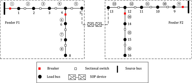
Figure 1. Topological diagram of a modified distribution network with two feeders (F1 and F2) interconnected by a soft open point (SOP).

Figure 2

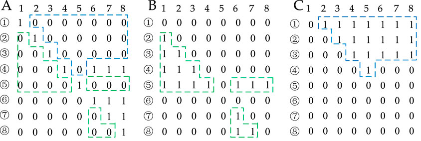
Figure 2. Schematic illustration of the fault impact matrices (A,B) and (C) corresponding to feeder F1 in Figure 1.

The lower-level model focuses on system reliability assessments by considering the fault scenarios, restoration processes, and time-varying load profiles comprehensively. Here, the EENS measured in kilowatt hour per year is adopted as the key reliability indicator and is calculated using the analytically derived expressions from the FIMs. To ensure model feasibility and accuracy, some essential operational constraints are incorporated, including unique restoration paths, SOP capacity limits, and network connectivity requirements.

2.2.1 Objective function

$\begin{array}{l}\min EENS\\ ={\displaystyle \sum _{l\in {\mathrm{\Omega }}^{\mathrm{L}}}}{\displaystyle \sum _{i\in {\mathrm{\Omega }}^{\mathrm{B}}}}{\lambda }_l\left(t_l^{\text{RE}}{a}_{li}^{\text{FIM}}+t^{\text{SW}}{b}_{li}^{\text{FIM}}+t^{\text{OP}}{\displaystyle \sum _{m=1}^{N^{\text{SOP}}}}{c}_{li,m}^{\text{FIM}}\right)E_i^{\mathrm{D}}\end{array},(39)$

$E_i^D=N^{\text{DAY}}{\displaystyle \sum _{s\in {\mathrm{\Omega }}^{\mathrm{S}}}}{p}_s{\displaystyle \sum _{t\in {\mathrm{\Omega }}^{\mathrm{T}}}}{P}_{i,s,t}^D\Delta t,\forall i\in {\mathrm{\Omega }}^{\mathrm{B}},(40)$

where ${\lambda }_l$ is the failure rate of line l; $t_l^{\text{RE}}$ is the repair time of line l; $t^{\text{SW}}$ is the switching time of the automatic sectionalizers on line l; $t^{\text{OP}}$ is the operation time of the SOP; $N^{\text{SOP}}$ is the total number of SOP devices in the system; $E_i^{\mathrm{D}}$ is the annual expected energy demand of node i; $a_{li}^{\text{FIM}}$ is a binary variable that is equal to 1 when the load at node i can only be restored by repairing the faulty branch l; $b_{li}^{\text{FIM}}$ is a binary variable that is equal to 1 when the load at node i can only be restored by automatic switching of line l; and $c_{li,m}^{\text{FIM}}$ is a binary variable that is equal to 1 when the load at node i can only be restored by the SOP after isolating the faulty line l. In Equation 39, the EENS is calculated via summation over all faulty branches. For each faulty branch, the corresponding outage duration is determined by the selected restoration strategy, which may include the repair time of the faulty line, automatic switching time, and/or SOP operation time. These durations are weighted by the failure rate of the branch and annual energy demand of the affected node. In Equation 40, the annual energy consumption at node i is defined as the weighted sum of hourly load demands in typical scenarios by taking into account the probability of each scenario.

2.2.2 Constraints

$a_{li}^{\text{FIM}}+b_{li}^{\text{FIM}}+{\displaystyle \sum _{m=1}^{N^{\text{SOP}}}}{c}_{li,m}^{\text{FIM}}\le 1,\forall l\in {\mathrm{\Omega }}^{\mathrm{L}},i\in {\mathrm{\Omega }}^{\mathrm{B}},(41)$

$\begin{array}{l}{\displaystyle \sum _{i\in {\mathrm{\Omega }}^{\mathrm{B}}}}{c}_{li,m}^{\text{FIM}}\left[{\left(P_{i,s,t}^D\right)}^2+{\left(Q_{i,s,t}^D\right)}^2\right]\le {\left(S_i^{\text{SOP}}\right)}^2\\ \forall l\in {\mathrm{\Omega }}^{\mathrm{L}},s\in {\mathrm{\Omega }}^{\mathrm{S}},t\in {\mathrm{\Omega }}^{\mathrm{T}},m\in \left[1,N^{\text{SOP}}\right]\end{array},(42)$

${\displaystyle \sum _{m=1}^{N^{\text{SOP}}}}{c}_{li,m}^{\text{FIM}}\le 1,\forall l\in {\mathrm{\Omega }}^{\mathrm{L}},i\in {\mathrm{\Omega }}^{\mathrm{B}},(43)$

$c_{li,m}^{\text{FIM}}\le c_{lo,m}^{\text{FIM}},\forall l\in {\mathrm{\Omega }}^{\mathrm{L}},i\in {\mathrm{\Omega }}^{\mathrm{B}},o\in {\mathrm{\Omega }}_i^{\text{SOP}},m\in \left[1,N^{\text{SOP}}\right],(44)$

$b_{li}^{\text{FIM}}\le b_{lq}^{\text{FIM}},\forall l\in {\mathrm{\Omega }}^{\mathrm{L}},i\in {\mathrm{\Omega }}^{\mathrm{B}},q\in {\mathrm{\Omega }}_i^{\text{SW}}.(45)$

Here, ${\mathrm{\Omega }}_i^{\text{SOP}}$ is the set of nodes on the restoration path from the substation to node i under a fault scenario and ${\mathrm{\Omega }}_i^{\text{SW}}$ is the set of nodes on the sectionalizing switch path from the substation to node i under a fault scenario. In Equation 41, each node is constrained to be restored by at most one method from among fault repair, switching operation, and SOP support; this formulation avoids overlapping restoration paths and eliminates ambiguity in the fault response. In Equation 42, an upper bound is imposed on the total apparent power delivered by a given SOP; accordingly, the sum of the real and reactive power demands of the restored loads must not exceed the rated capacity of the SOP unit. In Equation 43, each load node is assigned to at most one SOP for power restoration; this constraint prevents duplicate recovery and enforces a clear assignment logic to the SOP units. In Equation 44, the consistency of the SOP-based restoration path is guaranteed; if the SOP is installed at node i, all upstream intermediate nodes o along the restoration path must also be energized. In Equation 45, when a load is restored via the main grid, all upstream nodes along its sectionalizing switch path must also be restored to ensure radial integrity of the network.

2.3 Solution strategy

To achieve an optimal configuration of the ESSs while enhancing the economic efficiency, voltage security, and reliability of a rural distribution network, we propose a two-level iterative optimization framework. Here, the upper-level model determines the key planning decisions, including the siting and sizing of the ESSs and OLTCs, with auxiliary consideration of the SOPs; the lower-level model then evaluates the EENS under a set of predefined fault scenarios by determining whether each load point can be resupplied through one of several feasible strategies, namely branch repair, sectionalizing switch isolation, and SOP-assisted transfer. The lower-level model receives the SOP deployment decisions from the upper level and returns the computed EENS value for inclusion in the upper-level objective function. An iterative solution strategy is thus adopted to coordinate the interactions between the upper- and lower-level models. In each iteration, the upper-level model is solved to obtain a candidate planning scheme; this scheme is passed to the lower-level model to evaluate the reliability performance. The calculated EENS is then fed back to the upper-level objective function, and the process is repeated until convergence is achieved. The condition for iteration termination is that the calculated reliability index meets the requirements. The complete optimization framework was implemented in the AMPL modeling environment, and the mathematical models were solved using the Gurobi commercial solver that provides efficient support for large-scale convex programming problems involved in both models.

3 Results analysis

In this study, we used a modified 31-node distribution system to verify the effectiveness of the proposed coordinated planning approach integrating SOPs and ESSs while accounting for the OLTCs and flexible agricultural loads.

3.1 Parameter settings

The topology of the modified 31-node distribution system is illustrated in Figure 3, where S1, S2, and S3 denote the three substations. This system was modified by adding OLTCs in the substations and three candidate SOP locations (6–20, 8–26, and 11–13), in addition to integrating 10 distributed PV units to reflect high-penetration renewable access. The set of voltage levels is given by $\left\{35\text{\hspace{0.17em}kV},10\text{\hspace{0.17em}kV}\right\}$ . The PV units are located at nodes 11, 12, 13, 14, 16, 18, 21, 24, 26, and 27. The SOP investment cost is set at 30 (10,000 CNY/unit), and the energy storage investment cost is 15 (10,000 CNY/unit). The costs of electricity purchase, line losses, voltage violation penalty, and PV curtailment penalty are each valued at 0.65 CNY/kWh, while the PV generation cost is set to 0.25 CNY/kWh. The maximum and minimum voltage limits are defined as 1.06 p.u. and 0.94 p.u., respectively, with the OLTC parameters including a maximum tap position of 5, a nominal tap ratio of 1 p.u., and a tap-step percentage of 0.015. The efficiency of the ESS is set at 0.95, and the SOP power conversion loss coefficient is 0.2. All branches in the system are assumed to be identical with a failure rate of 0.05 failures per year per kilometer. The average repair time for a faulty branch is 3 h, while the switching operation times are 0.0002 h for the sectionalizing switches and 0.0017 h for the tie switches. We employed real residential load data from a representative weak rural distribution area. Several typical daily load profiles were selected as the scenario inputs to the optimization model, whose corresponding load curves are shown in Figure 4.

Figure 3

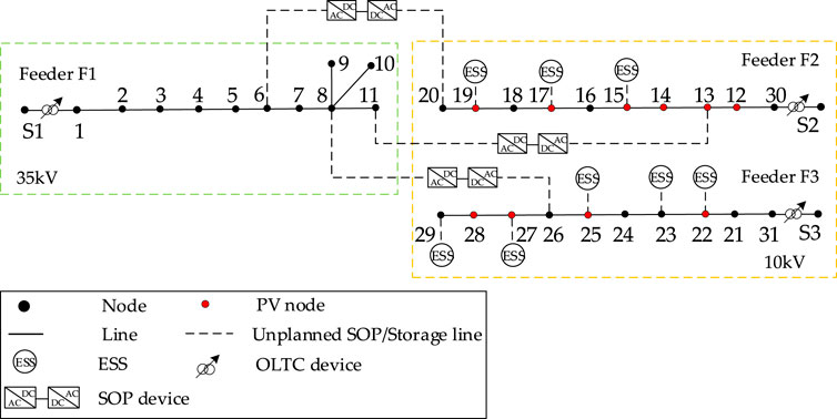
Figure 3. Configuration of the modified 31-node distribution network.

Figure 4

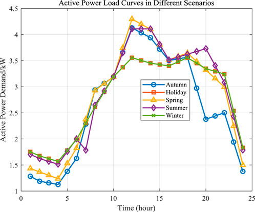
Figure 4. Representative daily load profiles for typical scenarios.

3.2 Analysis of the planning results

To assess the proposed coordinated planning method, three comparative cases were designed as follows:

• Case 1: No planning measures are implemented

• Case 2: SOP and ESS planning is carried out without OLTC regulation

• Case 3: SOP and ESS planning is combined with OLTC regulation.

3.2.1 Optimization results

The optimal planning configuration obtained using the proposed method is shown in Figure 5. Here, a single SOP device is installed between nodes 5 and 19 to manage the power flows and maintain voltage balance across different regions. In addition, two ESSs are deployed at nodes 14 and 18 to enhance system flexibility and improve operational reliability. The newly installed SOP and ESS units are highlighted in red in the figure. A comparative analysis of the total costs under different scenarios is presented in Table 1. In Case 1, the absence of investment planning leads to a high operating cost of 15.18587 billion RMB, resulting in significantly elevated overall cost. In Case 2, the coordinated planning of SOPs and ESSs reduces the operating costs to 12.45365 billion RMB, yielding a cost savings of approximately 2.732 billion RMB; this clearly illustrates the economic benefits achieved through optimization-based infrastructure investment. In Case 3, further incorporation of OLTC regulation leads to a marginal reduction in the operating cost to 12.45167 billion RMB and a total cost of 12.75167 billion RMB, reflecting a modest improvement in economic efficiency through enhanced voltage control.

Figure 5

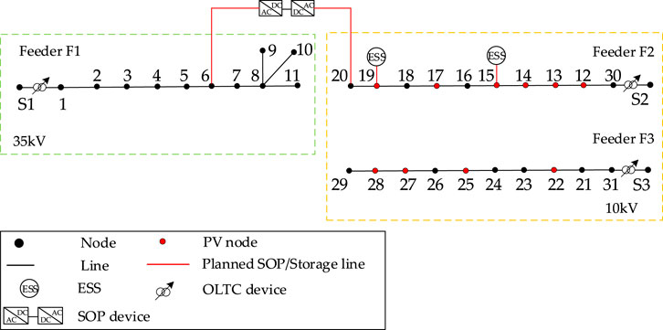
Figure 5. Optimal deployment scheme of the SOP and ESSs.

Table 1

Table 1. Comparison of the total costs under different planning scenarios.

3.2.2 Curtailment of PV generation

To further evaluate the effectiveness of the proposed planning method, Table 2 presents a comparison of PV generation curtailment for the three cases. In Case 1, where no flexible resources are deployed, the system exhibits a substantial PV curtailment of 30.876 MW, highlighting the limited capacities of traditional distribution networks to integrate high proportions of renewable generation. In Case 2, the deployment of SOPs and ESSs significantly reduces the curtailed PV power to 1.964 MW, indicating improved load accommodation capabilities. In Case 3, the introduction of OLTC regulation eliminates PV curtailment, enabling full utilization of renewable generation. These results confirm that coordinated deployment of SOPs and ESSs enhances the renewable energy hosting capacity of the distribution network. Moreover, the integration of OLTC control provides further benefits with regard to voltage regulation. Thus, the proposed method demonstrates practical effectiveness in accommodating high levels of PV integration in rural distribution systems.

Table 2

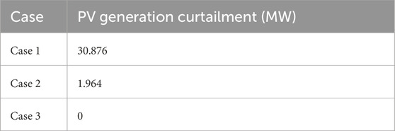
Table 2. PV generation curtailment under different cases.

3.3 Reliability assessment

Table 3 summarizes the EENS results under two different planning scenarios at both the 35 kV and 10 kV levels. In Case 1, where flexible resources such as SOPs or ESS are absent, the system exhibits relatively high EENS values of 169.260 MWh/year at the 35 kV feeder and 124.850 MWh/year at the 10 kV feeder. These figures reflect the limited fault-tolerance capabilities of conventional radial topologies, where supply interruptions caused by faults cannot be mitigated efficiently. In Case 2, the coordinated deployment of SOPs and ESSs leads to significant reductions in the EENS values, which decrease to 72.508 MWh/year at the 35 kV feeder and 20.839 MWh/year at the 10 kV feeder. This reduction is particularly evident at the 10 kV level, where the EENS decreases by approximately 83%, highlighting the positive impacts of flexible resources in ensuring supply continuity for rural end-users. Note that the difference between Case 3 and Case 2 lies in the presence of OLTCs. However, both cases result in the same planning outcome, which has no impact on the EENS. These results confirm the effectiveness and practicality of the proposed integrated planning strategy for rural distribution networks.

Table 3

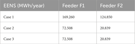
Table 3. Expected energy not supplied (EENS) results under different cases.

4 Conclusion

A two-level optimization planning method is proposed for rural distribution systems that integrate ESSs, OLTCs, SOPs, and rural flexible loads within a two-level optimization framework. The simulation results verify the effectiveness of the proposed method, and the following conclusions can be drawn:

1. The integration of SOPs and ESSs significantly reduces PV curtailment and enhances renewable energy utilization. The simulation results show that compared to the case without SOPs and ESSs, the curtailed PV output is reduced from 30.876 MW to 1.964 MW and further eliminated when combined with OLTC control.

2. OLTC regulation effectively enhances the voltage control capacity of the distribution system to enable full absorption of renewable energy without additional investment. The results demonstrate excellent cost-effectiveness under high penetration conditions.

3. The proposed method improves the system reliability and operational flexibility. The simulation results show that the proposed method reduces the EENS by more than 50% at both feeders F1 and F2 as well as the total cost by approximately 16%.

Future research efforts will focus on detailed modeling of the selector and divertor switches of the OLTCs and their applications in the planning model. Moreover, we intend to investigate resilience-oriented planning strategies to address extreme-weather and climate challenges in the future.

Data availability statement

The raw data supporting the conclusions of this article will be made available by the authors without undue reservation.

Author contributions

XY: Methodology, Writing – review and editing, Conceptualization. YZ: Data curation, Writing – review and editing. FZ: Data curation, Writing – review and editing. RX: Formal Analysis, Writing – original draft, Writing – review and editing. FJ: Writing – original draft, Formal Analysis, Writing – review and editing. JX: Visualization, Software, Writing – review and editing, Validation.

Funding

The authors declare that financial support was received for the research and/or publication of this article. This work is supported by the Science and Technology Project of State Grid Anhui Electric Power Co., Ltd. (No. B3120924000C). The funder was involved in providing technical guidance and project background information during the research process.

Acknowledgements

The authors are grateful to the Science and Technology Project of State Grid Anhui Electric Power Co., Ltd for the funding.

Conflict of interest

Authors XY, YZ, FZ, and RX were employed by the Economic and Technological Research Institute of State Grid Anhui Electric Power Co., Ltd.

Authors FJ and JX were employed by Anhui Mingsheng Hengzhuo Technology Co., Ltd.

Generative AI statement

The authors declare that no Generative AI was used in the creation of this manuscript.

Any alternative text (alt text) provided alongside figures in this article has been generated by Frontiers with the support of artificial intelligence and reasonable efforts have been made to ensure accuracy, including review by the authors wherever possible. If you identify any issues, please contact us.

Publisher’s note

All claims expressed in this article are solely those of the authors and do not necessarily represent those of their affiliated organizations, or those of the publisher, the editors and the reviewers. Any product that may be evaluated in this article, or claim that may be made by its manufacturer, is not guaranteed or endorsed by the publisher.

References

Cheng, J. (2021). “Capacity evaluation of agricultural irrigation load participating in sustainable power and energy operating reserve of power system,” in 202l IEEE conference (iSPEC). Nanjing, China, 2511–2517. doi:10.1109/iSPEC53008.2021.9735435

CrossRef Full Text | Google Scholar

Cheng, S., Wei, Z., Shang, D., Zhao, Z., and Chen, H. (2020). Charging load prediction and distribution network reliability evaluation considering electric vehicles’ spatial-temporal transfer randomness. IEEE Access 8, 124084–124096. doi:10.1109/ACCESS.2020.3006093

CrossRef Full Text | Google Scholar

Diao, H., Li, P., Tu, C., and Che, L. (2025). Optimal co-planning of multi-port soft open points and energy storage systems for improving hosting capacity and operation efficiency in distribution networks. IEEE Trans. Power Deliv. 40 (1), 459–471. doi:10.1109/TPWRD.2024.3503662

CrossRef Full Text | Google Scholar

Fu, X., Bai, J., Sun, H., and Zhang, Y. (2024). Optimizing agro-energy-environment synergy in agricultural microgrids through carbon accounting. IEEE Trans. Smart Grid 15 (5), 4819–4834. doi:10.1109/TSG.2024.3397990

CrossRef Full Text | Google Scholar

Guo, H., Wang, Q., Wang, Y., Liu, S., Tang, L., and Li, L. (2022). “Capacity allocation of energy storage system improving high penetration renewable energy accommodation,” in 2022 5th international conference on power and energy applications (ICPEA). Guangzhou, China, 504–509. doi:10.1109/ICPEA56363.2022.10052291

CrossRef Full Text | Google Scholar

Ji, H., Wang, C., Li, P., Ding, F., and Wu, J. (2019). Robust operation of soft open points inactive distribution networks with high penetration of photovoltaic integration. IEEE Trans. Sustain. Energy 10 (l), 280–289. doi:10.1109/TSTE.2018.2833545

CrossRef Full Text | Google Scholar

Jiang, X., Zhou, Y., Ming, W., Yang, P., and Wu, J. (2022). An overview of soft open points in electricity distribution networks. IEEE Trans. Smart Grid 13 (3), pp1899–pp1910. doi:10.1109/TSG.2022.3148599

CrossRef Full Text | Google Scholar

Jooshaki, M., Abbaspour, A., Fotuhi-Firuzabad, M., Muñoz-Delgado, G., Contreras, J., Lehtonen, M., et al. (2020). Linear formulations for topology-variable-based distribution system reliability assessment considering switching interruptions. IEEE Trans. Smart Grid 11 (5), 4032–4043. doi:10.1109/TSG.2020.2991661

CrossRef Full Text | Google Scholar

Li, R., Wang, W., and Xia, M. (2018). Cooperative planning of active distribution system with renewable energy sources and energy storage systems. IEEE Access 6, 5916–5926. doi:10.1109/ACCESS.2017.2785263

CrossRef Full Text | Google Scholar

Li, Z., Wu, W., Tai, X., and Zhang, B. (2020). Optimization model based reliability assessment for distribution networks considering detailed placement of circuit breakers and switches. IEEE Trans. Power Syst. 35 (5), 3991–4004. doi:10.1109/TPWRS.2020.2981508

CrossRef Full Text | Google Scholar

Li, B., Qin, C., Yu, R., Dai, W., Shen, M., Ma, Z., et al. (2023). Fast solution method for the large-scale unit commitment problem with long-term storage. Chin. J. Electr. Eng. 9 (3), 39–49. doi:10.23919/CJEE.2023.000033

CrossRef Full Text | Google Scholar

Li, W., Zou, Y., Yang, H., Fu, X., Xiang, S., and Li, Z. (2025). Two-stage stochastic energy scheduling for multi-energy rural microgrids with irrigation systems and biomass fermentation. IEEE Trans. Smart Grid 16 (2), 1075–1087. doi:10.1109/TSG.2024.3483444

CrossRef Full Text | Google Scholar

Lin, L., Jia, Q., Lv, C., Liang, J., and Luo, P. (2023). Partitional collaborative mitigation strategy of distribution network harmonics based on distributed model predictive control. IEEE Trans. Smart Grid 14 (3), 1998–2009. doi:10.1109/TSG.2022.3211008

CrossRef Full Text | Google Scholar

Liu, W., Lin, Z., Wang, L., Wang, Z., Wang, H., and Gong, Q. (2020). Analytical reliability evaluation of active distribution systems considering information link failures. IEEE Trans. Power Syst. 35 (6), 4167–4179. doi:10.1109/TPWRS.2020.2995180

CrossRef Full Text | Google Scholar

Pamshetti, V. B., and Singh, S. P. (2022). Coordinated allocation of BESS and SOP in high PV penetrated distribution network incorporating DR and CVR schemes. IEEE Syst. J. 16 (1), 420–430. doi:10.1109/JSYST.2020.3041013

CrossRef Full Text | Google Scholar

Pamshetti, V. B., Singh, S., Thakur, A. K., Singh, S. P., Babu, T. S., Patnaik, N., et al. (2023). Cooperative operational planning model for distributed energy resources with soft open point in active distribution network. IEEE Trans. Ind. Appl. 59 (2), 2140–2151. doi:10.1109/TIA.2022.3223339

CrossRef Full Text | Google Scholar

Pan, G., Gu, W., Lu, Y., Qiu, H., Lu, S., and Yao, S. (2020). Optimal planning for electricity hydrogen integrated energy system considering power to hydrogen and heat and seasonal storage. IEEE Trans. Sustain. Energy 1l (4), 2662–2676. doi:10.1109/TSTE.2020.2970078

CrossRef Full Text | Google Scholar

Peng, Y., Yang, Y., Chen, M., Wang, X., Xiong, Y., Wang, M., et al. (2023). Value evaluation method for pumped storage in the new power system. Chin. J. Electr. Eng. 9 (3), 26–38. doi:10.23919/CJEE.2023.000029

CrossRef Full Text | Google Scholar

Qian, Y., Wang, H., Zhou, M., Lv, H., and Liu, Y. (2022). Frequency trajectory planning-based frequency regulation strategy for wind turbines equipped with energy storage system. Chin. J. Electr. Eng. 8 (2), 52–61. doi:10.23919/CJEE.2022.000014

CrossRef Full Text | Google Scholar

Qiao, J., Meng, X., Zheng, W., Huang, P., Xu, T., and Xu, Y. (2025). Optimization configuration method of energy storage considering photovoltaic power consumption and source-load uncertainty. IEEE Access 13, 9401–9412. doi:10.1109/access.2025.3528050

CrossRef Full Text | Google Scholar

Ravikumar, R., Srinivasan, M. V., Karunakaran, R. V., Srikanth, A., and Vijayaraghavan, V. (2022). “Deferrable irrigation load optimization in rural microgrid clusters,” in 2022 IEEE conference on technologies for sustainability (SusTech). Corona, CA, USA, 125–131. doi:10.1109/SusTech53338.2022.9794162

CrossRef Full Text | Google Scholar

Saaklayen, M. A., Shabbir, M. N. S. K., Liang, X., Faried, S. O., and Janbakhsh, M. (2023). A two-stage multi-scenario optimization method for placement and sizing of soft open points in distribution networks. IEEE Trans. Ind. Appl. 59 (3), 2877–2891. doi:10.1109/TIA.2023.3245588

CrossRef Full Text | Google Scholar

Schum, S., and Lin, A. (2012). China's renewable energy law and its impact on renewable power in China: progress, challenges and recommendations for improving implementation. Energy Policy 5l, 89–109. doi:10.1016/j.enpol.2012.06.066

CrossRef Full Text | Google Scholar

Tao, A., Zhou, N., Chi, Y., Wang, Q., and Dong, G. (2023). Multi-stage coordinated robust optimization for soft open point allocation in active distribution networks with PV. J. Mod. Power Syst. Clean Energy 1l (5), 1553–1563. doi:10.35833/MPCE.2022.000373

CrossRef Full Text | Google Scholar

Timalsena, K. R., Piya, P., and Karki, R. (2021). A novel methodology to incorporate circuit breaker active failure in reliability evaluation of electrical distribution networks. IEEE Trans. Power Syst. 36 (2), 1013–1022. doi:10.1109/TPWRS.2020.3010529

CrossRef Full Text | Google Scholar

Wang, C., Zhang, T., Luo, F., Li, P., and Yao, L. (2018). Fault incidence matrix based reliability evaluation method for complex distribution system. IEEE Trans. Power Syst. 33 (6), 6736–6745. doi:10.1109/TPWRS.2018.2830645

CrossRef Full Text | Google Scholar

Wei, W., Zhou, Y., Zhu, J., Hou, K., Zhao, H., Li, Z., et al. (2019). Reliability assessment for AC/DC hybrid distribution network with high penetration of renewable energy. IEEE Access 7, 153141–153150. doi:10.1109/ACCESS.2019.2947707

CrossRef Full Text | Google Scholar

Wei, W., Ye, Z., Wang, Y., Dai, S., Chen, L., and Liu, X. (2022). An economic optimization method for demand-side energy-storage accident backup assisted deep peaking of thermal power units. Chin. J. Electr. Eng. 8 (2), 62–74. doi:10.23919/CJEE.2022.000015

CrossRef Full Text | Google Scholar

Xiang, Y., Su, Y., Wang, Y., Liu, J., and Zhang, X. (2020). An explicit formula based estimation method for distribution network reliability. IEEE Trans. Power Deliv. 35 (4), 2109–2112. doi:10.1109/TPWRD.2019.2949887

CrossRef Full Text | Google Scholar

Yan, J., Liu, S., Yan, Y., Liu, Y., Han, S., and Zhang, H. (2024). How to choose mobile energy storage or fixed energy storage in high proportion renewable energy scenarios: evidence in China. Appl. Energy 376, 124274. doi:10.1016/j.apenergy.2024.124274

CrossRef Full Text | Google Scholar

Yin, H., Wang, Z., Liu, Y., Qudaih, Y., Liu, D. T., Liu, J., et al. (2023). Operational reliability assessment of distribution network with energy storage systems. IEEE Syst. J. 17 (1), 629–639. doi:10.1109/JSYST.2021.3137979

CrossRef Full Text | Google Scholar

Zhang, H., Luo, Y., Fang, S., Niu, T., Yang, J., and Liao, R. (2025). Coordinated energy carbon management for agricultural integrated energy system. IEEE Trans. Ind. Appl. 6l (3), 4603–4612. doi:10.1109/TIA.2025.3532908

CrossRef Full Text | Google Scholar