Experimental data on mechanical impact in non-oriented electrical steel magnetic characteristics

1 Introduction

Improving the efficiency of electrical machines requires a detailed understanding of how ferromagnetic materials behave under mechanical stress. One critical phenomenon in this context is magneto-mechanical coupling, in which mechanical stresses caused, either during manufacturing processes such as cutting, drilling, stacking, and shrink fitting (Bernard et al., 2011; Bernard and Daniel, 2015; Miyagi et al., 2009; M'zali et al., 2021; Nakata et al., 1992; Schoppa et al., 2000; Rygal et al., 2000; Wang et al., 2023), or during operation due to inertial forces (Coey, 2010; Landgraf, 2016; Leuning et al., 2023), affect the magnetic response of the material. Such stresses can lead to anisotropy and alter key magnetic properties, including permeability and energy losses.

To investigate these effects, a custom magneto-mechanical test bench was developed to impose controlled uniaxial mechanical stress while simultaneously applying a magnetic field (Mailhé, 2018; Mailhé et al., 2020). The resulting dataset provides experimental measurements that capture how mechanical loading influences the magnetic behavior of non-oriented electrical steel sheets. These measurements form a reliable foundation for studying magneto-mechanical coupling, validating constitutive models, and supporting simulation-based design of electrical machines.

The dataset presented here serves as an open experimental resource for the scientific community. This article provides a foundation for studying magneto-mechanical coupling, validating constitutive models, and supporting the design of electrical machines through simulations. Crucially, the specialized magneto-mechanical test bench used is custom-built and not commercially available. By providing this data publicly, the dataset offers researchers who may lack access to such experimental facilities the opportunity to conduct their own in-depth analyses.

2 Experimental setup and instruments

The experimental setup is centered on a custom-built magneto-mechanical test bench, incorporating instruments including a Mecmesin® universal testing machine for applying mechanical loads (tension and compression at 5, 10, 15, and 20 MPa levels), H-coil sensors for direct magnetic field measurement, and a National Instruments® NI-6212 data acquisition system controlled via a LabVIEW virtual instrument (VI).

The primary instrument for data acquisition is the custom-built magneto-mechanical test bench, a modified Single Sheet Tester (SST) designed to apply uniaxial stresses parallel to the magnetic flux direction. This specialized setup allows for the study of magnetic material behavior under tensile or compressive mechanical stresses. Figure 1 illustrates the system: Figure 1A) shows a view of the test bench and the modified SST, highlighting the mechanical application components. Figure 1B presents the functional diagram of the system, detailing the control circuit, the power excitation components, and the measurement loops.

Figure 1

Figure 1. Magneto-mechanical test bench: illustration and functional diagram. (A) Illustration of Magneto-mechanical bench (Modified SST) with emphasis on the SST and the anti-buckling case. (B) Functional diagram of the test bench, including the control and excitation components (Mailhé et al., 2020).

The magneto-mechanical test bench comprises three main interconnected blocks: I) the modified SST with mechanical stress application, II) magnetic induction waveform control, and III) signal amplification, filtering, and data acquisition. These blocks operate in an integrated manner to apply controlled mechanical and magnetic conditions while enabling precise signal acquisition.

Block I: the modified SST with mechanical stress application consists of a ferromagnetic core (two C-shaped pieces) enclosing a primary winding (700 turns) and a secondary winding (375 turns). The electrical steel sample is positioned within an anti-buckling structure to maintain its shape under compressive loads. The entire SST assembly is integrated into a Mecmesin® universal tensile/compression machine, which applies uniaxial forces measured by a dynamometer with a reading capacity of up to 2500 N (Figure 1A). The modified SST is enclosed in a box with a thin sheet (≈0, 02 mm) of amorphous-ferrous steel providing external electromagnetic shielding. The influence of shielding on this bench was previously investigated by Mailhé et al. (2018).

Block II: the magnetic induction waveform control block is responsible for generating the magnetic flux imposed on the samples and regulating the voltage in the secondary winding of the modified SST. A control bench previously developed at GRUCAD (Batistela, 2001) and detailed at Figure 1B) is used to maintain a sinusoidal induced voltage waveform, representing the time derivative of magnetic induction. This is achieved through a nonlinear sliding mode control algorithm operating in closed loop, which ensures stable waveform fidelity across different loading conditions.

Block III: the signal amplification, filtering, and data acquisition block is responsible for amplifying voltage signals from the magnetic field sensors and acquiring all necessary signals for calculating the magnetic quantities of interest. Magnetic field measurement is performed indirectly using three H-coil sensors. These sensors have cross-sectional areas on the order of 5 × 10⁻⁵ m² yielding induced voltages in the range of 0.7 µV RMS to 20 µV RMS at 1 Hz. Signal amplification is implemented with a gain factor of 1,035 to ensure accurate capture of low-voltage signals. The data acquisition is conducted using a National Instruments® NI-6212 board connected via USB to a dedicated LabVIEW virtual instrument, which also performs preliminary signal visualization and logging.

2.1 Samples

The samples consist of NOG iron-silicon (Fe-Si) electrical steel sheets cut in three different directions relative to the rolling direction: 0° (RD), 45° (DD), and 90° (TD). The dimensions of the characterized samples are detailed in Table 1. Dimensional data were obtained by averaging at least three measurement sets.

Table 1

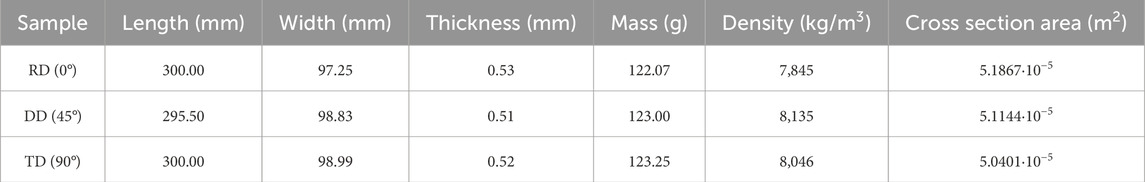
Table 1. Samples information.

3 Data acquisition methodology

The σ-H test methodology was implemented to investigate the effects of mechanical stress on the magnetic characteristics of the material, focusing on inverse magnetostriction (Villari effect). This methodology involves first applying mechanical stress (σ) to the sample and then performing magnetic measurements (magnetic field H).

The experimental procedure consisted of two phases: (i) mechanical stress configuration and (ii) magnetic excitation. Uniaxial tensile and compressive stresses of 5, 10, 15, and 20 MPa, as well as a no-stress condition (0 MPa), were applied. The applied force was regulated by adjusting the displacement of the Mecmesin® universal testing machine.

For magnetic excitation, sinusoidal magnetic induction waveforms were imposed at 1 Hz, 50 Hz, and 100 Hz. The peak induction levels were increased in 0.05 T steps, ranging from 0.05 T to a target maximum of 1.5 T. Samples were demagnetized before each set of experiments. Signal waveforms were monitored using an oscilloscope to ensure waveform fidelity throughout the test.

3.1 Data processing

Signal acquisition included the excitation voltage, excitation current (using a 100 mV/A probe), secondary winding voltage, and the three amplified H-coil sensor voltages. Data collection and initial waveform inspection were managed using a LabVIEW Virtual Instrument.

For data processing, magnetic induction $B\left(t\right)$ was calculated by integrating the secondary winding voltage $v_s$ as shown in (Equation 1). In this equation, $N_s$ is the is the number of turns of the secondary winding and S is the cross-sectional area of the sample.

$B\left(t\right)={\int }_0^t-\frac{1}{N_{s}S}{v}_s\left(t^{\prime }\right)d{t}^{\prime }(1)$

Magnetic field strength $H\left(t\right)$, presented in (Equation 2), was determined by integrating the voltages $v_H$ from the three H-coil sensors at three known distances from the material samples. In this equation $N_H$ and$S_H$ are, respectively, the number of turns (2000 turns) and the cross-sectional area ($\approx {3,210}^{-5}m{m}^2$) of each H-coil winding. The constant ${\mu }_0$ is the magnetic permeability of free space ($4\pi {10}^{-7}$ H/m).

$H_{coil}\left(t\right)=\frac{1}{N_H{S}_H{\mu }_0}{\int }_0^t{v}_H\left(t^{\prime }\right)d{t}^{\prime }(2)$

The magnetic field at the surface of the sample, denoted as Hextrap in the dataset, was determined using an extrapolation procedure applied to measurements obtained from three H-coil sensors. This approach is based on the principle of tangential field continuity across media with differing magnetic permeabilities in the absence of surface currents (Bastos and Sadowski, 2016).

The magnetic energy loss per unit volume (J/m³), is estimated based on the ferromagnetic material BH characteristic. The area of the BH loop was numerically calculated using both ∫H dB and ∫B dH approaches. Integrations were performed using the trapezoidal rule across discrete data points in both loops and the results were averaged to minimize numerical discrepancies. The energy loss (J/kg) was calculated by dividing the volumetric energy loss by the sample density.

3.1.1 Magnetic field acquisition: indirect vs. extrapolated method

A common strategy for calculating the magnetic field used to determine BH curves is the indirect method (Equation 3), which measures the field based on the primary coil current. In this methodology, the magnetic field $H_i\left(t\right)$ is calculated from the waveform of the excitation current $i\left(t\right)$, the number of turns of the primary winding $N_p$, and the mean magnetic path length of the magnetic circuit $l_m$.

$H_i\left(t\right)=\frac{N_p}{l_m}i\left(t\right)(3)$

This test bench, however, exhibited significant limitations with this approach, which were investigated in Mailhé (2018). The primary issue is that the indirect method compromises data accuracy primarily because the low magnitude of the magnetizing current often generates excessive noise during the 1 Hz measurements. Furthermore, as both frequency and induction increase, anomalies become evident. These unexpected behaviors are attributed to two potential physical causes: either a possible resonance within the RLC circuit formed by the primary coil and the magnetizing components, or the existence of short-circuits between yoke laminations inducing interlaminar losses.

Given these observed limitations and the necessity for a more in-depth investigation into the underlying physical phenomena, the reliability of the extrapolated field approach was confirmed by validating the results by comparison with tests performed on the same material samples using the Brockhaus® test bench (under no-stress conditions). This validation process, which was carried out specifically for the data presented here and is detailed in (Silva, 2019), led to the selection of the extrapolated field method from the H-coil sensors as the exclusive basis for obtaining all magnetic field values in this dataset.

3.2 Data description

The dataset is organized in a hierarchical directory structure, as illustrated in the flowchart of Figure 2. In this chart, positive values (+5 MPa, +10 MPa, +15 MPa and +20 MPa) represent tensile stress, whereas negative values ($-$ 5 MPa, $-$ 10 MPa, $-$ 15 MPa and $-$ 20 MPa) represent compression stress.

Figure 2

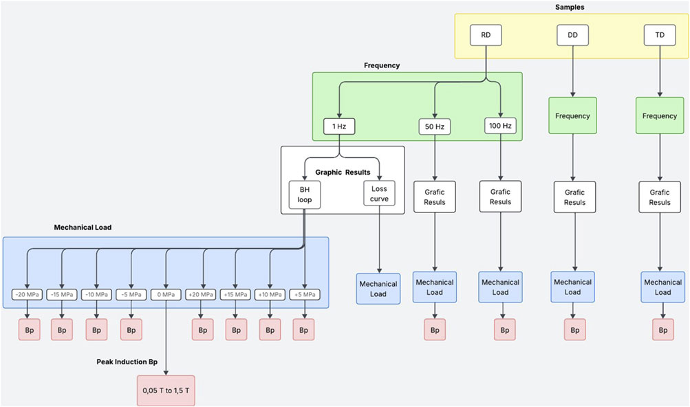
Figure 2. Data organization flowchart.

This structure was designed to facilitate the visualization and analysis of magnetic characteristics, such as BH loops and magnetic loss curves. Each box in the diagram corresponds to a subfolder, with the lowest level containing individual data files in CSV format.

The main directory, titled Magneto-mechanical_Coupling_Data, contains three primary subfolders, each representing a sample orientation: RD_Sample, DD_Sample, and TD_Sample. Within each of these, the data are subdivided by test frequency: 1 Hz, 50 Hz, and 100 Hz. Each frequency folder includes two types of data: BH_loop (instantaneous magnetic induction and field strength) and loss_curve (magnetic loss values in J/kg).

The BH_loop folder includes nine subfolders, each corresponding to a specific mechanical stress level and type. The folder names encode both the stress intensity (ranging from 0 MPa to 20 MPa) and the stress type, using the prefix “T” for tensile and “C” for compressive stress. For example, the directories RD_Sample/1Hz/BH_loop/T5 MPa and RD_Sample/1Hz/BH_loop/C5 MPa contain BH loop data under +5 MPa and $-$ 5 MPa, respectively. This pattern is repeated across all sample orientations and frequencies, enabling easy navigation in the dataset and locate BH loop data for any given mechanical condition.

Each subfolder of BH loop in a specific mechanical stress condition contains CSV files with 10,000 time-series data points each (corresponding to one full cycle). The first column represents the instantaneous magnetic field strength in the sample Hextrap(t) in A/m, and the second column the instantaneous magnetic induction B(t) in T. The file names follow a consistent pattern that includes the peak induction value (Bp, in mT), the frequency, and the variables involved in the folder, as shown in the example: Bp_150 mT_1Hz_H-EXTRAPvsB.csv.

Similarly, the loss_curve folder also includes nine CSV files, each corresponding to a distinct stress condition. Each file reports the magnetic loss (second column, in J/kg) as a function of peak induction (first column, in T) for the given sample and frequency. For example, RD_Sample/1Hz/loss_curve contains magnetic loss data for the nine stress levels tested at 1 Hz. A specific file such as RD_Losses_0 MPa_1Hz.csv provides 30 measurements under zero-stress conditions. File names follow the same logic for other stress levels, with the stress value and type embedded accordingly.

This structure enables multifactorial analysis of magnetic behavior as a function of sample orientation, mechanical stress, and excitation frequency. A Python-based script is included in the dataset to automate the visualization of BH loops and loss curves. The user can select input parameters (sample orientation, frequency, and stress level) and generate corresponding plots. Figure 3A illustrates a representative BH loop obtained for the RD sample at the four compressive level applied and the no-stress condition, 1 Hz and 1,000 mT, while Figure 3B shows the variation of hysteresis loss (losses at 1 Hz) with increasing peak induction for the RD sample for the same stress condition presented in Figure 3A. This visualization demonstrates the strong impact of compressive stresses, evidencing intense modifications in the BH loops and, consequently, in magnetic losses, due to the sharp decrease in magnetic permeability. The curves, presented in red, green, orange, and blue, illustrate the changes caused by the compression levels of $-$5, $-$10, $-$15, and $-$20 MPa, respectively, contrasting with the purple reference curve for the no-stress condition.

Figure 3

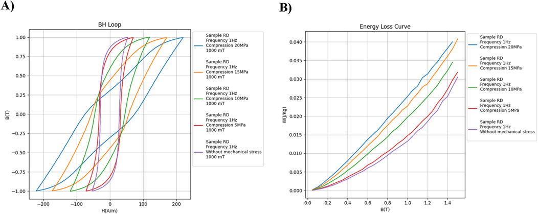
Figure 3. Examples of analysis with the dataset. (A) Loss curve of RD sample at 1 Hz, compression levels and no-stress condition. (B) Loss curve of RD sample at 1 Hz, compression levels and no-stress condition.

3.3 Limitations

The ability to achieve higher peak magnetic induction levels was constrained by the limitations of the experimental setup. This restriction occurs primarily at high magnetic inductions and under compressive mechanical stress because the magneto-mechanical coupling effect significantly modifies the BH curves. This alteration leads to a considerable increase in the material’s dissipated magnetic losses, consequently demanding a higher current excitation from the test bench. Table 2 presents the maximum peak induction values achieved for each sample under different frequency and mechanical stress conditions.

Table 2

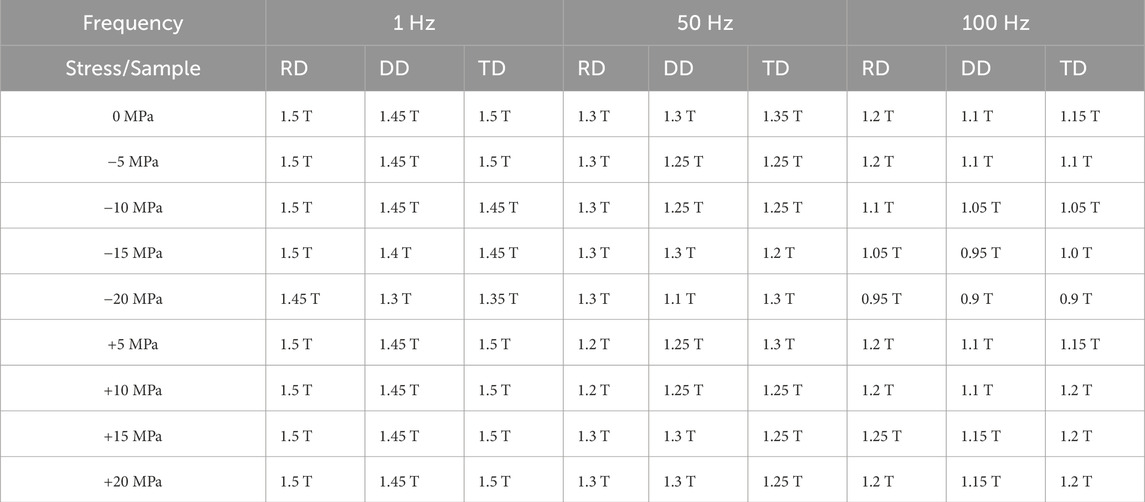
Table 2. Maximum peak induction values achieved.

Additionally, intrinsic magnetic and metallurgical variations among the samples such as differences in grain structure, texture, or chemical composition may have introduced slight inconsistencies. Dimensional tolerances in thickness and cutting accuracy could also have contributed to minor discrepancies in the measured results. Nevertheless, these variations are within acceptable ranges typically observed for non-oriented electrical steel sheets.

Data availability statement

The datasets presented in this study can be found in online repositories. The names of the repository/repositories and accession number(s) can be found at: http://doi.org/10.17632/hgzgpcvjxk.

Author contributions

IPCS: Data curation, Investigation, Writing – original draft, Validation, Formal Analysis. GFMN: Visualization, Writing – review and editing. YGL: Software, Visualization, Writing – review and editing. NJB: Project administration, Methodology, Writing – review and editing, Validation, Supervision, Conceptualization. NS: Supervision, Methodology, Writing – review and editing, Conceptualization, Validation. JVL: Writing – review and editing, Resources.

Funding

The author(s) declare that financial support was received for the research and/or publication of this article. We acknowledge the financial support provided by CAPES (Brazilian Coordination for the Improvement of Higher Education Personnel), CNPq (Brazilian National Council for Scientific and Technological Development) and FINEP (Brazilian Studies and Project Financer under grant 2072/23 “Development of an electrification system for onboard hydraulic devices in utility vehicles”) for financing this project over several years.

Acknowledgments

The authors would also like to thank the Federal University of Santa Catarina (UFSC) for supporting this research.

Conflict of interest

The authors declare that the research was conducted in the absence of any commercial or financial relationships that could be construed as a potential conflict of interest.

Generative AI statement

The author(s) declare that no Generative AI was used in the creation of this manuscript.

Any alternative text (alt text) provided alongside figures in this article has been generated by Frontiers with the support of artificial intelligence and reasonable efforts have been made to ensure accuracy, including review by the authors wherever possible. If you identify any issues, please contact us.

Publisher’s note

All claims expressed in this article are solely those of the authors and do not necessarily represent those of their affiliated organizations, or those of the publisher, the editors and the reviewers. Any product that may be evaluated in this article, or claim that may be made by its manufacturer, is not guaranteed or endorsed by the publisher.

References

Bastos, J. P. A., and Sadowski, N. (2016). Magnetic materials and 3D finite element modeling. Boca Raton: CRC Press. doi:10.1201/b15558

CrossRef Full Text | Google Scholar

Batistela, N. J. (2001). Caracterização e modelagem eletromagnética de lâminas de aço ao silício. Doctoral dissertation. Brazil: Federal University of Santa Catarina. Available online at: http://repositorio.ufsc.br/xmlui/handle/123456789/81963.

Google Scholar

Bernard, L., and Daniel, L. (2015). Effect of stress on magnetic hysteresis losses in a switched reluctance motor: application to stator and rotor shrink fitting. IEEE Trans. Magnetics 51, 1–13. doi:10.1109/TMAG.2015.2435701

CrossRef Full Text | Google Scholar

Bernard, L., Mininger, X., Daniel, L., Krebs, G., Bouillault, F., and Gabsi, M. (2011). Effect of stress on switched reluctance motors: a magneto-elastic finite-element approach based on multiscale constitutive laws. IEEE Trans. Magnetics 47, 2171–2178. doi:10.1109/TMAG.2011.2145387

CrossRef Full Text | Google Scholar

Coey, J. M. D. (2010). Magnetism and magnetic materials. Cambridge University Press. doi:10.1017/CBO9780511845000

CrossRef Full Text | Google Scholar

Landgraf, F. J. G. (2016). Propriedades magnéticas de aços para fins elétricos. São Paulo: Blucher.

Google Scholar

Leuning, N., Schauerte, B., and Hameyer, K. (2023). Interrelation of mechanical properties and magneto-mechanical coupling of non-oriented electrical steel. J. Magnetism Magnetic Mater. 567, 170322. doi:10.1016/j.jmmm.2022.170322

CrossRef Full Text | Google Scholar

M'zali, N., Henneron, T., Benabou, A., Martin, F., and Belahcen, A. (2021). Finite element analysis of the magneto-mechanical coupling due to punching process in electrical steel sheet. IEEE Trans. Magnetics 57 (6), 7401304. doi:10.1109/TMAG.2021.3058310

CrossRef Full Text | Google Scholar

Mailhé, B. J. (2018). Characterization and modelling of the magnetic behaviour of electrical steel under mechanical stress. Doctoral dissertation. Brazil: Federal University of Santa Catarina. Available online at: https://repositorio.ufsc.br/handle/123456789/198679.

Google Scholar

Mailhé, B. J., Elias, R. A., da Silva, I. P. C., Sadowski, N., Batistela, N. J., and Kuo-Peng, P. (2018). Influence of shielding on the magnetic field measurement by direct H-Coil method in a double-yoked SST. IEEE Trans. Magnetics 54 (3), 1–4. doi:10.1109/TMAG.2017.2758959

CrossRef Full Text | Google Scholar

Mailhé, B. J., Bernard, L. D., Daniel, L., Sadowski, N., and Batistela, N. J. (2020). Modified-SST for uniaxial characterization of electrical steel sheets under controlled induced voltage and constant stress. IEEE Trans. Instrum. Meas. 69 (12), 9756–9765. doi:10.1109/TIM.2020.3006682

CrossRef Full Text | Google Scholar

Miyagi, D., Maeda, N., Ozeki, Y., Miki, K., and Takahashi, N. (2009). Estimation of iron loss in motor core with shrink fitting using FEM analysis. IEEE Trans. Magnetics 45, 1704–1707. doi:10.1109/tmag.2009.2012790

CrossRef Full Text | Google Scholar

Nakata, T., Nakano, M., and Kawahara, K. (1992). Effects of stress due to cutting on magnetic characteristics of silicon steel. IEEE Transl. J. Magn. Jpn. 7, 453–457. doi:10.1109/TJMJ.1992.4565422

CrossRef Full Text | Google Scholar

Rygal, R., Moses, A. J., Derebasi, N., Schneider, J., and Schoppa, A. (2000). Influence of cutting stress on magnetic field and flux density distribution in non-oriented electrical steels. J. Magnetism Magnetic Mater. 215-216, 687–689. doi:10.1016/S0304-8853(00)00259-6

CrossRef Full Text | Google Scholar

Schoppa, A., Schneider, J., Wuppermann, C. D., and Bakon, T. (2000). Influence of welding and sticking of laminations on the magnetic properties of non-oriented electrical steels. J. Magnetism Magnetic Mater. 254-255, 367–369. doi:10.1016/S0304-8853(02)00877-6

CrossRef Full Text | Google Scholar

Silva, I. P. C. (2019). Estudos sobre o efeito dos esforços mecânicos no comportamento de valores de parâmetros de modelos de perdas magnéticas. Master's thesis. Brazil: Federal University of Santa Catarina. Available online at: https://repositorio.ufsc.br/handle/123456789/215634.

Google Scholar

Wang, S., Wang, Y., Liu, C., Lei, G., Guo, Y., and Zhu, J. (2023). Performance comparison of tubular flux-switching permanent magnet machines using soft magnetic composite material and hybrid material magnetic cores. IEEE Trans. Energy Convers. 38 (2), 1118–1129. doi:10.1109/TEC.2023.3235992

CrossRef Full Text | Google Scholar