Verification of the PWR core solver coupling the neutron code nTRACER with artificial neural networks for thermal–hydraulic feedback

The Paul Scherrer Institute (PSI) and North Carolina State University are developing a high-resolution multi-physics core solver for pressurized water reactor (PWR) analysis in Cartesian geometry, using the neutron transport code nTRACER and two machine learning (ML) models providing thermal–hydraulic (T/H) feedback. This work presents the coupling of nTRACER/ML, comparing the solver with the verified core solver nTRACER/CTF, in terms of accuracy and computation costs, for steady-state and cycle analysis, with the presented results and their interpretation focusing primarily on performance improvements. nTRACER/ML shows strong agreement with nTRACER/CTF in power and coolant predictions for hot full power, with maximum deviations of 1.01% in assembly power and 2.63 °C in coolant temperature (root mean square error [RMSE]: 0.65 °C). Fuel temperature predictions are also good, with centerline temperature differences reaching up to 32.96 °C and an RMSE of 5.55 °C. As exposure increases, power deviations grow up to 3.33% axially and 4.13% in 3D assembly power at 392.3 effective full power days (EFPDs). Coolant temperature discrepancies decrease with burnup, while fuel temperature errors increase, with centerline differences peaking at 36.24 °C (RMSE: 8.30 °C). Despite its limitations, nTRACER/ML shows sufficient agreement with nTRACER/CTF in both neutronic and T/H metrics, making it a practical low-fidelity alternative for high-resolution simulations, particularly because it runs 3–4 times faster than CTF while using only approximately 1% of the CPU time.

1 Introduction

Modeling plays a fundamental role throughout the nuclear power plant (NPP) lifecycle, from design to operation and decommissioning. Verified and validated multi-physics computational tools are essential to predict critical parameters, such as parameters relevant to reactor core behavior. Conventional neutronics calculates parameters on a detailed subset of the geometry, which are then used in a separate code for a simplified full-core neutron balance. These neutronic codes are coupled with T/H solvers of comparable resolution, enabling assembly-level core analysis and coarse reactor pressure vessel (RPV) modeling. All the involved approximations often lead to conservative operational limits (D’Auria, 2019). This approach is being re-evaluated by the nuclear industry, considering an alternative based on the calculation of the best estimated value of those parameters, complemented with uncertainty limits (BEPU). Advances in computing now allow the use of high-resolution, multi-physics codes for pin- or sub-pin-level neutronics and subchannel T/H analysis. These high-fidelity codes enable more tightly coupled, first-principles modeling of safety parameters (e.g., fuel temperature) at local scales, capturing heterogeneities like Chalk River unidentified deposit (CRUD) formation that conventional tools approximate or omit. With reduced approximations and high-resolution information, novel codes can improve the estimation of core conditions and identify potential issues like fuel rod failure (Clifford et al., 2019). Thus, they support BEPU by reducing unnecessary conservatism in safety margins, allowing more efficient and flexible fuel and reactor use (Avramova et al., 2021). Novel codes can be proven critical for challenges like power uprates, lifetime extensions, higher burnup, and for optimizing performance and safety in current and future reactors. This shift is key for nuclear energy competitiveness in meeting policy demands for lower costs and flexible systems (IAEA, 2017). Such code systems for the multi-physics high-resolution simulation of the reactor core in pressurized water reactors (PWRs) are VERA, Serpent/Subchanflow, and nTRACER/CTF (Kochunas et al., 2017; García et al., 2021; Kwon et al., 2025).

Despite all the associated benefits, the computational cost of novel core solvers limits their use in routine production calculations. It is significantly larger than the cost of the conventional approach, demanding large computing clusters (Papadionysiou et al., 2022). Integrating novel high-resolution solvers into standard safety analysis can be supported by auxiliary low-cost solvers that approximate secondary phenomena in the reactor core with reduced fidelity but equivalent resolution. For example, neutronic phenomena primarily govern core behavior and fuel depletion in a PWR under normal operation, while T/H phenomena, involving single-phase coolant with axially dominated flow, are easier to model. A high-resolution solver can handle the primary phenomena, coupled with a lower-fidelity auxiliary solver for secondary effects. While the combined solutions are less accurate than full high-fidelity tools (Pap et al., 2022), they can serve as reliable guidelines, reducing the need for extensive multi-physics calculations, provided the auxiliary solver maintains sufficient accuracy to avoid significant discrepancies in the high-resolution solver. Machine learning (ML) methods offer a promising way to develop auxiliary solvers, as they can handle complex problems with a few parameters by finding patterns in data. Through large dataset analysis, ML models can predict outcomes and uncover new insights. Applications of ML in nuclear energy include power operations, maintenance planning, reactor design, regulatory tools, risk analysis, and fuel management (Delipei et al., 2023; Song and Kim, 2024; Agarwal et al., 2022; Ramos et al., 2024). Despite challenges to its adoption, ML simplifies complex problems, enabling better decision-making and contributing to safer, more efficient, and economically competitive nuclear power.

The Laboratory of Reactor Physics and Thermal-Hydraulics (LRT) has developed a multi-physics computational tool for the simulation of the Cartesian core with the latest version of the 3D sub-pin neutron transport code nTRACER and the subchannel code COBRA-TF (CTF) for high-resolution cycle analysis (Kwon et al., 2025; Pap et al., 2024). nTRACER was developed by Seoul National University (SNU) and has been verified with international PWR benchmarks (Ryu et al., 2015). CTF is being jointly developed by North Carolina State University (NCSU) and Oak Ridge National Laboratory (ORNL) and has been verified and validated for PWR steady-state and transient analysis (Spasov et al., 2017). The coupled code system has been verified for cycle analysis in LRT on the framework of the OECD/NEA Tennessee Valley Authority (TVA) Watts Bar 1 (WB1) benchmark (Albagami et al., 2022). This includes several exercises for code-to-code verification and validation with experimental data using novel high-fidelity multi-physics computational tools. At the same time, LRT, in collaboration with NCSU, is developing a second high-resolution multi-physics core solver for Cartesian PWR analysis with nTRACER and two ML models for the calculation of the coolant and fuel properties, respectively, to have an alternative option with smaller computational costs than nTRACER/CTF. In addition to being verified extensively for PWRs, nTRACER is capable of neutronic analysis at the sub-pin level with lower computational costs than Monte Carlo codes and comparable accuracy (Papadionysiou, 2022). For these reasons, it is considered suitable to be coupled with ML models. Both ML models, ML-CTF-Cool (Papadionysiou et al., 2025a) and ML-CTF-Fuel (Papadionysiou et al., 2025b), are built with artificial neural networks (ANNs), based on the T/H analysis of CTF for a PWR during normal operation. ANNs are chosen for the ML models because the underlying physical phenomena are highly complex and benefit from deep learning approaches. A preliminary study using polynomial expansions to calculate the fuel temperature profile demonstrated the need for high-order ML models. Other methods, such as convolutional neural networks (CNNs) and random forests, may also be suitable and will be explored in future work. The TVA WB1 benchmark is used as a basis for the development of the two ML models and the verification of nTRACER/ML. The benchmark is designed for the verification and validation of high-resolution multi-physics core solvers and has already been used for the verification of nTRACER/CTF (Kwon et al., 2025). ML-CTF-Cool and ML-CTF-Fuel have been verified with standalone CTF calculations for the whole range of operating conditions corresponding to the three depletion cycles described in the benchmark specifications. ML methods to provide high-resolution full-core T/H feedback to a sub-pin neutronic code for cycle analysis have not been attempted before, to the extent of the authors’ knowledge. The motivation behind this work is to develop a high-resolution multi-physics core solver for low-fidelity analysis with smaller computational costs than nTRACER/CTF. This tool can be very useful for studies requiring many calculations with approximate results to approach the optimal range, like optimization studies or uncertainty and sensitivity analysis, which then can be explored by nTRACER/CTF with high-fidelity calculations. In the future, nTRACER could also be replaced by an ML model. There are already data-driven tools for neutronic analysis like RAPID (He and Walters, 2020).

This work focuses on the verification of nTRACER/ML with nTRACER/CTF for the hot full power (HFP) state and the first cycle of TVA WB1. The article begins by presenting all computational tools and methods involved in the study (Section 2). The coupling scheme of nTRACER/ML is described in detail, together with all differences in the capabilities of the two code systems (Section 3). TVA WB1 is also briefly presented with the relevant nTRACER/ML models (Section 4). The HFP case of the benchmark is used to verify nTRACER/ML vs. nTRACER/CTF and also to quantify the impact of the different approximations involved in the ML models on the accuracy of the coupled solution (Section 5.1). Finally, the nTRACER/ML results for the first cycle of TVA WB1 are presented and verified at specific exposure points with nTRACER/CTF (Section 5.2). The relevant computational costs of the T/H solvers are compared in Section 5.3.

2 Code and tool description

This section is focused on the description of the codes, solvers, and ML models used for the simulation of the 3D core, together with the coupling scheme between nTRACER and the ANNs providing T/H feedback.

2.1 nTRACER

nTRACER is a direct deterministic transport code capable of solving the neutron transport equation at the sub-pin level while considering the full extent of the reactor geometry. The code is based on a 2D/1D scheme with 3D acceleration, considering a heterogeneous description of the reactor core. Cross-sections are calculated on the fly (47 energy groups) using the subgroup method for resonance treatment. nTRACER has its own cross-section library built by SNU, which is based on ENDF/B.VII.0. The explicit modeling of the nuclide and temperature distributions inside each fuel pellet is required. The code divides the 3D core into separate axial layers or planes, which are modeled explicitly. The planar (2D) transport equation is solved with the method of characteristics (MOC), and then the different planes are coupled through the neutron axial leakage source (1D). The axial leakage is calculated by a 3D coarse mesh Finite difference (CMFD) formulation, which includes different 1D axial solvers, like SP3, and specifically, 1D MOC for the latest version of nTRACER (Choi and Joo, 2020). The flux and cross-sections of the MOC planes are homogenized to create the 3D CMFD problem, and the radial leakage source is calculated. The radial and axial solutions are coupled by the corresponding transverse leakage terms, forming a 3D problem. The purpose of the CMFD formulation is to combine the 2D/1D scheme and accelerate the MOC calculations. nTRACER employs hybrid parallelization methods [message passing interface (MPI) and OpenMP] with an axial domain decomposition (one MPI per axial plane). The default scattering treatment is transport-corrected P0. However, there is the option for higher orders. For depletion calculations, nTRACER uses its own depletion library, built by SNU and the predictor–corrector scheme. The Bateman equation is solved with the flux at the beginning of the burnup (BU) step (predictor), defining a new material composition. The cross-sections, corresponding to the new material composition, are used to perform a state-point neutronic calculation and predict the flux distribution. The new flux is used to recalculate the material composition of the BU step (corrector). The average of the isotopic densities calculated by the predictor and the corrector steps is considered the material composition at the end of the BU step. In the typical predictor–corrector scheme with linear interpolation, a second state-point neutronic calculation would take place with the averaged material composition. nTRACER also includes a simplified predictor–corrector approach, where the transport calculation after the corrector step is omitted, resulting in a drastic reduction (nearly half) of the calculation time and a solution of lower accuracy. The typical predictor–corrector is used in this study.

2.2 CTF

CTF (Salko and Avramova, 2015) is a subchannel T/H code developed for analyzing light water reactor (LWR) vessels and cores. It employs a two-fluid model with three distinct fields, each governed by its own set of conservation equations. This study focuses on PWRs during normal operation, with single-phase, axially dominated coolant flow. CTF uses parallel channels defined by fuel rods and open gaps, divided into axial intervals based on model geometry. These subchannels form a 3D computational mesh, in which the mass, energy, and momentum conservation equations are solved using a staggered mesh approach. Scalar quantities are computed at the control volume centers, while velocity fields are calculated at the surfaces. CTF models detailed energy, mass, and momentum transfer (crossflow) between subchannels, treating lateral flow without fixed coordinates, as all directions orthogonal to the vertical axis are considered. This assumption holds for axially dominated flow with minimal crossflow and momentum transfer. The conservation equations and pressure matrix are solved simultaneously, enabling the calculation of parameters like pressure gradients and fuel rod temperatures. CTF calculates fuel rod temperature profiles with sub-pin resolution and models key fuel behavior aspects, including temperature-dependent material properties and gap conductance. Concerning depletion calculations, CTF is equipped with models that take into account local BU in material properties and can simulate basic structural changes caused by depletion, such as fuel swelling leading to gap closure. The code is parallelized using the MPI standard with radial domain decomposition.

2.3 Artificial neural networks

An ANN (et and Hastie, 2009) is composed of interconnected neurons, organized into an input layer, an output layer, and one or more hidden layers. Neurons in each layer connect to adjacent layers via weighted edges. Each neuron applies a nonlinear activation function to signals received from the previous layer and transmits the output to the next layer. The weights, which control signal strength, allow the network to learn complex functions through its hidden layers. Training an ANN involves optimizing weights to minimize the difference between predicted and real values in a training dataset. This process uses two types of parameters: network parameters, such as weights, which are updated during training, and hyperparameters, which define the network’s architecture and training process and are set beforehand. Training proceeds iteratively, starting with a forward pass to compute outputs for a batch of data, followed by error calculation using a loss function. The error is then backpropagated to adjust the weights through an optimization algorithm, guided by the learning rate, a critical hyperparameter for weight updates (Goodfellow et al., 2017). As training advances, the model’s accuracy improves. To ensure the generalization capability of ANNs, the dataset is split into two parts: one used for both training and hyperparameter optimization, and a separate one reserved for final testing. Within the training phase, k-fold cross-validation is applied to optimize the hyperparameters and assess the model’s performance more reliably. This approach helps mitigate overfitting and ensures that the trained ANN performs consistently across a range of input conditions, while the independent test set provides an unbiased evaluation of the model’s predictive accuracy.

2.3.1 ML-CTF-Cool

ML-CTF-Cool (Papadionysiou et al., 2025a) aims to predict coolant properties, specifically temperature and density, with subchannel resolution, independently for each subchannel in the active core. It must be pointed out that the methodology designed for the development of ML-CTF-Cool can be applied to different PWR cores, to produce ML models capable of high-resolution T/H predictions with relatively low computational cost (Papadionysiou et al., 2025a). However, ML-CTF-Cool is developed specifically for TVA WB1. The subchannel on which the ML model is applied is hereafter referred to as the subchannel of interest (SOI). Regarding axial discretization, a fixed, uniform mesh is used with a node size of approximately 5 cm, which is sufficiently fine to capture all local variations. Spacer grids are also not considered in developing the ML model. Their influence is not considered critical for steady-state analysis; however, their effect on the accuracy of the code solver is studied in Section 5.1. The parameters that are used as features for the ML model are selected among the outputs of nTRACER (or any coupled neutronic code), the geometric characteristics of the core, and the reactor’s global operating conditions. At the same time, the flow-related effects of subchannels not close to the SOI are considered to be encompassed in the influence of their direct neighbors (see Figure 1). The 4 × 4 lattice containing the SOI and its eight neighbors is therefore defined as the region of interest with which all predictors selected for the ML model are associated. These predictors are

• ${HS}_k={\displaystyle {\sum }_{i=1}^{fuelpins}}{wp}_{i,k}{f}_{rad,i}{f}_{ax,i}{q}^{\prime }{A}_k$, for k = 1–9, referring to the SOI and its eight neighbors (see Figure 1). ${wp}_{i,k}$ is the fraction of the wetted perimeter of each fuel pin i that is connected to subchannel $k$ (${wp}_{i,k}=0.25$ in Cartesian geometry). $f_{rad,i}$ and $f_{ax,i}$ are the peaking factors of the radial and axial power profile corresponding to fuel pin i, and $q^{\prime }$ the global linear heat generation rate.

• A logical predictor determining if any of the subchannels of the region of interest belong to the inter-assembly gap.

• A logical predictor determining if any of the subchannels of the region of interest belong to the inter-assembly gap corner.

• The number of subchannels in the 4 × 4 region of interest that are delimited by GTs.

• The coolant temperature of the axial node below the SOI. This means that the prediction for axial node j is based on the prediction of coolant temperature for axial node j−1, except for the first axial node, which uses the core inlet temperature $T_{in}$.

Figure 1

Figure 1. Spatial visualization of ${HS}_k$ for the SOI and its eight neighbors.

Due to the last predictor, ML-CTF-Cool predicts the coolant properties for all subchannels of an axial layer simultaneously through vectorization and then proceeds to the next axial layer. The model is trained with data from CTF calculations. A database of 4,620,000 samples is created, 20% of which are used for testing. The architecture of ML-CTF-Cool is presented in Table 3. The ReLU activation function is applied to all units. All relevant hyperparameters for the training and the architecture of the model are selected with five-fold cross-validation. More detailed information for the training of the model can be found in Papadionysiou et al. (2025a). As mentioned in Section 1, ML-CTF-Cool has been verified against CTF for different operating conditions that cover the whole range of normal operation of TVA WB1 for the three cycles described in the benchmark. Table 1 presents the range of applicability for ML-CTF-Cool, which fully covers the actual core power distribution of TVA WB1 (Papadionysiou et al., 2025a). The verification cases also include varying mass flux and the exclusion of the water liner between the active core and the core barrel. To tackle the effect of mass flux, two formulas have been derived to correct the predictions of ML-CTF-Cool. The formulas are presented and verified by Papadionysiou et al. (2025a) and used in this work. The water liner between the active core and the core baffle is excluded from the geometries that comprise the database used to train ML-CTF-Cool. Its effect proves insignificant according to the relevant studies performed by Papadionysiou et al. (2025a). Nonetheless, the impact of excluding the water liner in the coupled solution is studied in Section 5.1. For all verification cases, ML-CTF-Cool never exceeds 4 $°C$ of maximum temperature difference and 2 $°C$ of root mean square error (RMSE), which is defined as the target accuracy (Papadionysiou et al., 2025a), presenting overall good agreement with CTF.

Table 1

Table 1. Range of applicability of ML-CTF-Cool.

2.3.2 ML-CTF-Fuel

ML-CTF-Fuel (Papadionysiou et al., 2025b) is trained with data from CTF calculations to predict the fuel temperature at the centerline and surface of each fuel pin, together with the cladding temperature at the inner and outer surface. ML-CTF-Fuel and the process used to build the ML model are both specifically designed for TVA WB1. Concerning axial discretization, the ML model is using a uniform fixed mesh with a node size of ∼5 cm. The fuel sub-pin temperature profile is reconstructed for each fuel pin with the following function:

$T\left(r\right)=T_{centerline}-\left(T_{centerline}-T_{surface}\right)·{\left(\frac{r}{fuel\_radius}\right)}^p,$

where r is the radius of the calculation pin and p is the parameter defining the shape of the radial profile. Normally, the parabolic function, for which p = 2, is considered appropriate for steady-state conditions in PWRs, considering constant gap conductivity, as discussed by Tong and Weisman (1979). However, in this work, p is set as 1.78, following a sensitivity study conducted on the CTF calculation for the HFP case of TVA WB1 (Kwon et al., 2025). The effect of parameter p and its selected value on the accuracy of the results when exposure takes place is further discussed in Section 5. The cladding temperature is assumed to be a linear function of radius, and the gap temperature is approximated as the average between the fuel surface temperature and the temperature of the cladding at its inner surface (Papadionysiou, 2022). ML-CTF-Fuel is trained specifically for TVA WB1. Table 2 presents the range of applicability for ML-CTF-Fuel. The parameters used as input features for the ML model are selected from the outputs of nTRACER (or any coupled neutronic code) and the coolant properties, which in this study are provided by ML-CTF-Cool. These predictors are

• $q_{pin}^{\prime }=f_{rad,pin}{f}_{ax,pin}{q}^{\prime }$, where $f_{rad,pin}$ and $f_{ax,pin}$ are the peaking factors of the radial and axial power profile corresponding to the specific fuel pin and $q^{\prime }$ is the global linear heat generation rate.

• The local BU for the specific fuel pin ${BU}_{pin}$.

• The temperature of the coolant surrounding the specific fuel pin $T_{bulk}$.

Table 2

Table 2. Range of applicability of ML-CTF-Fuel.

Spacer grids are again not considered for the development of the ML model. Their effect is studied in Section 5.1. The model is trained with data from CTF calculations. A database of 1,260,000 samples is created, 20% of which are used for testing. The architecture of ML-CTF-Fuel is presented in Table 3. The ReLU activation function is applied to all units. All relevant hyperparameters for the training and the architecture of the model are selected with five-fold cross-validation. More detailed information for the training of the model can be found in Papadionysiou et al. (2025b). ML-CTF-Fuel has been verified with CTF quarter core simulations based on the TVA WB1 benchmark. The temperature difference does not exceed 1.4 °C for the cladding and 14.55 °C for the fuel, with the RMSE reaching a maximum of 3.47 °C for the centerline temperature, indicating a good agreement between the ML model predictions and CTF.

Table 3

Table 3. Architecture of ML-CTF-Cool and ML-CTF-Fuel.

3 nTRACER/ML coupling scheme

Because nTRACER is programmed with Fortran and the ML tools are programmed with Python, an external coupling scheme is developed with a Python wrapper. Figure 2 presents the calculation scheme of nTRACER/ML. The process for a single state-point simulation is the following:

1. nTRACER processes the relevant input, and after completing the first CMFD calculation, it initiates the sequence for T/H feedback. It creates the CTF input decks as it would for an nTRACER/CTF calculation (Kwon et al., 2025; Pap et al., 2024) and produces two text files containing the local power and BU for each pin. Finally, it calls the Python wrapper to be executed externally.

2. The Python wrapper begins by processing all information provided by nTRACER. It reads the geometry model from the CTF input decks, together with other parameters that are important for the T/H calculation, such as mass flux. Then, after reading the relevant text files, it stores the local power and BU and transforms the data from the axial mesh of the neutronic code to the axial mesh of the ML tools. If an ML mesh axial node is fully contained in an nTRACER axial node, it is assigned the same local power and BU as the corresponding nTRACER axial node. If it is lying between two different nTRACER axial nodes, the local power and BU are calculated as the weighted average of the values for the two nTRACER axial nodes.

3. The Python wrapper employs ML-CTF-Cool to calculate the subchannel temperature and density with the provided input data. As mentioned in Section 2.3.1, ML-CTF-Cool predicts the coolant properties for all subchannels of an axial layer simultaneously through vectorization and then proceeds to the next axial layer. The coolant properties of the pin cell are calculated as the weighted average of the values corresponding to the four subchannels surrounding the fuel pin (Cartesian geometry) and transformed to the nTRACER axial mesh. The outlet temperature of the core is also calculated as the area-weighted average of the subchannel temperature at the top axial node of the ML model. Finally, the pin cell temperature and density is printed in a text file, following the numbering scheme of nTRACER, and the outlet temperature in a separate text file.

4. The Python wrapper proceeds with the calculations of the fuel temperature profile. The local BU and power, provided by nTRACER, are used together with the predicted pin cell coolant temperature by ML-CTF-Fuel to predict the pin centerline, surface, inner cladding, and outer cladding temperatures simultaneously for all pins through vectorization. The predictions are transformed to the nTRACER axial mesh and printed in a text file, following the nTRACER numbering scheme. This concludes the function of the Python wrapper.

5. nTRACER processes the three text files produced by the Python wrapper and calculates the temperature profile for each pin according to the methodology described in Section 2.3.2. Then, the code updates its cross-sections and proceeds to the MOC calculation, and after the next CMFD iteration. As long as the T/H solution is not converged (the change in the pin average fuel temperature is smaller than 10⁻⁴ (Papadionysiou et al., 2022)), nTRACER updates the local power and BU information after each CMFD iteration and calls the Python wrapper.

Figure 2

Figure 2. nTF/CTF depletion calculation scheme for BU step k.

The calculation process described above corresponds to a single state point. As mentioned by Kwon et al. (2025) and Papadionysiou et al. (2022), the PSI HPC cluster Merlin6 is used to perform the nTRACER/CTF calculations. The same cluster is also used for nTRACER/ML. Merlin6 limits the simulation time for a single calculation to under 24 h. This constraint does not allow the simulation of an entire operating cycle with a single calculation. The same depletion scheme that was applied on nTRACER/CTF to tackle this issue, Kwon et al. (2025) and Papadionysiou et al. (2022), is also used for nTRACER/ML. Each BU step of the operating cycle is simulated independently of the previous and next BU step, with the use of a restart file, which is created after the completion of each BU step. A simulation that uses restart files requires two state-point calculations per BU step. For BU step k, the first state-point calculation is performed with the material composition of BU step k−1, which is the averaged material properties from the respective predictor and corrector calculations of BU step k−1, and the new operating conditions. Then, the second state-point calculation uses the flux calculated at the first state point to further deplete the material composition to the designated exposure of step k with the simplified predictor–corrector. Therefore, the depletion calculation scheme of nTRACER/CTF and nTRACER/ML operates as a full predictor–corrector.

4 TVA WB1 benchmark

The “OECD/NEA TVA Watts Bar Unit 1 Multi-Physics Multi-Cycle Depletion” benchmark (Albagami et al., 2022) is based on the real plant data of the first three cycles of the Tennessee Valley Authority (TVA) Watts Bar Nuclear Unit 1 (WB1). The benchmark contains a detailed description of the reactor core and includes hot zero power (HZP) start-up tests, an HFP steady-state (beginning of cycle) code-to-code comparison, and three depletion cycles with fuel reshuffling. Figure 3 presents the fuel enrichment and poison loading patterns for the fresh core in quarter symmetry, which corresponds to the HFP steady state and the first cycle. Figure 4 illustrates the simplified power history of the first cycle. Together with the power history, the evolution of all core operating conditions, like the position of the control rods and the inlet temperature, is provided in the benchmark specification as a function of BU. The benchmark team also provided LRT with the measured boron curve for the first cycle. As mentioned in Section 1, the nTRACER/ML results for the first cycle of TVA WB1 are presented and verified at specific exposure points with nTRACER/CTF. These points are also marked on Figure 4. Their selection is discussed further in Section 5.2.

Figure 3

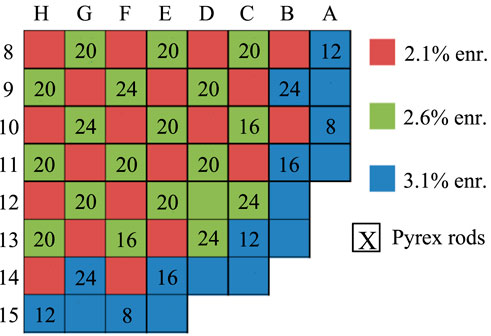
Figure 3. Fresh fuel radial enrichment and poison loading patterns in the quarter core.

Figure 4

Figure 4. Power history for the first cycle of TVA WB1.

4.1 nTRACER/ML TVA WB1 models

As mentioned in Section 1, nTRACER has been verified for the HZP start-up tests (Pap et al., 2024), and nTRACER/CTF has been verified for the HFP steady state and the first depletion cycle (Kwon et al., 2025). In this work, nTRACER/ML is verified with nTRACER/CTF for the HFP state and the first cycle of TVA WB1. The nTRACER/ML models are based on the nTRACER/CTF models presented by Kwon et al. (2025). All involved approximations are listed below, together with the differences in the CTF simulations and the ML tools. Figure 5 presents some of the applied geometry approximations on the nTRACER model.

• The axial reflectors are homogenized in nTRACER (see Figure 5A) to introduce axial nodes of sufficient height to avoid calculation instabilities (Kelley, 2015). In CTF, the axial reflectors are modeled as additional axial layers of the active core with zero power. On the other hand, ML-CTF-Cool does not provide predictions of coolant properties in the axial reflector region. It is assumed that the moderator temperature and density at the outlet of the active core can also characterize the plenum and top reflector region.

• Previous work with nTRACER (Ryu et al., 2015) has proven that the radial reflector model can exclude the reactor pressure vessel, extending only until the outer diameter of the neutron pads, with negligible impact on the nTRACER solution. The core shroud is modeled explicitly; however, the core barrel and the neutron pads are approximated by homogenized pin cells of water and steel (see Figure 5B). A water gap is modeled between the reflector assemblies because nTRACER defines a uniform inter-assembly gap with the same size and material for the whole core. The CTF model includes the water liner between the active core and the shroud, which is not taken into account by ML-CTF-Cool. Nonetheless, Papadionysiou et al. (2025a) demonstrated that the effect on accuracy is not significant.

• In nTRACER, the spacer grids are modeled as rings around the cladding of each rod, conserving the total mass and volume of the actual spacer grid (see Figure 5C). In the case of instrumentation or guide tubes, the spacer grid material density is increased to conserve the mass, so that the diameter of the spacer grid ring does not surpass the limits of the pin cell. The axial height of each spacer grid is double the actual height designated in the benchmark specification, while maintaining the same volume, to ensure the stability of the nTRACER simulation. CTF models the spacer grids as loss coefficients according to the benchmark specification. The ML tools do not consider spacer grids. This will be studied further in Section 5.1.

• The inserted control rods are not modeled in the plenum region in nTRACER. They are fully excluded by CTF and the ML tools. Nonetheless, the effect is not significant (Kwon et al., 2025).

• In Kwon et al. (2025), the detector thimbles are modeled by nTRACER/CTF in specific locations according to the benchmark specifications. In this work, these are excluded in nTRACER/CTF and nTRACER/ML because the ML tools do not take them into account.

Figure 5

Figure 5. Approximations of the nTRACER model for the TVA WB1 core.

5 Results

As discussed in Section 1 and by Papadionysiou et al. (2025a) and Papadionysiou et al. (2025b), nTRACER/ML is intended to be used as a low-fidelity, multi-physics solver. In addition, this work is a preliminary study to pinpoint sources of discrepancy and bottlenecks in the coupling scheme between nTRACER and the two ML models. Thus, specific accuracy criteria for the local power and temperature are not defined at this point in the study to characterize the performance of the low-fidelity solver. The accuracy of nTRACER/ML throughout the cycle analysis is compared with the discrepancies presented in the nTRACER/CTF vs. VERA verification for the equivalent cases, when higher discrepancies emerge.

5.1 HFP

The HFP steady state described in TVA WB1 (Exercise 2) utilizes the fresh fuel loading pattern shown in Figure 3. The inlet temperature is 291.85 °C, and one control rod bank is partially inserted at the top of the core. Xenon is modeled in equilibrium in both core solvers. The benchmark specifies that 2.6% of the total heat is deposited directly into the coolant. This direct heating effect is accounted for in CTF and ML-CTF-Fuel but is neglected in ML-CTF-Cool, as it has minimal impact on local coolant properties (Papadionysiou et al., 2025a).

As noted in Sections 2.3.1, 4.1, the ML models were not trained with configurations that included spacer grids or the water liner surrounding the active core. Three verification test cases are defined to assess the impact of these approximations on solution accuracy:

• Case 0: Designed to ensure a consistent comparison between nTRACER/CTF and nTRACER/ML, this case is based on the TVA WB1 HFP model but excludes spacer grids from both neutronic and T/H calculations. The active core is discretized into 22 equally sized axial nodes. The water liner is included in nTRACER for both solvers but is not modeled in CTF.

• Case 1: Here, spacer grids are introduced in the nTRACER model for both solvers, as well as in CTF. Consequently, the axial discretization is no longer uniform, following the spacer grid model described in Section 4.1. The water liner is included in the neutronic calculations but is still neglected in CTF.

• Case 2: Here, nTRACER/ML is verified vs. the nTRACER/CTF model for the TVA WB1 HFP case outlined in Section 4.1, incorporating both the spacer grids and the water liner, which are also included in the nTRACER calculation.

Figure 6 presents the absolute difference of the axially averaged pin power of nTRACER/CTF vs. nTRACER/ML, [${power}_{nTRACER/CTF}-{power}_{nTRACER/ML}$], for Cases 0 and 2. Figure 7 presents the normalized axial power profile as it is calculated from both core solvers for Cases 0 and 2, together with the relevant absolute difference. The solution of Case 1 is not included in the two figures because it is very similar to Case 2. Table 4 summarizes the maximum absolute difference and RMSE of the 3D assembly power, the axially averaged pin power, the axial power profile, and the critical boron concentration (CBC) as calculated by nTRACER/CTF and nTRACER/ML for all cases.

Figure 6

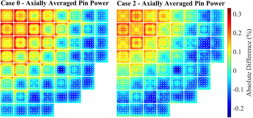
Figure 6. Absolute difference of the axially averaged pin power of nTRACER/CTF vs. nTRACER/ML for Cases 0 and 2.

Figure 7

Figure 7. Normalized axial power profile as calculated by nTRACER/CTF and nTRACER/ML for Cases 0 (left) and 2 (right) together with their absolute difference.

Table 4

Table 4. Maximum absolute difference and RMSE of the nTRACER/CTF solution vs. nTRACER/ML for the 3D assembly power, axially averaged pin power (2D), and axial power profile (1D) for all test cases.

By analyzing Figures 6, 7 alongside Table 4, it becomes evident that nTRACER/ML demonstrates strong agreement with nTRACER/CTF for both global and local quantities. The CBC difference remains consistently at approximately 4 ppm across all cases. Discrepancies in assembly power and axial profile become more pronounced as the spacer grids and water liner are introduced into the models. The maximum observed differences reach 1.01% for assembly power and 0.72% for axial power—both well within acceptable limits. Additionally, the RMSE of absolute differences does not exceed 0.40% for either quantity across all cases. The axially averaged pin power distributions also show strong agreement, with a maximum absolute difference of 0.31% and an RMSE of approximately 0.10% for all cases. Pin power discrepancies remain relatively stable across different cases. This suggests that the introduction of spacer grids and the water liner primarily impacts the axial power distribution, as seen in Figure 7. The shape of the axial power difference profile remains consistent across all cases, becoming more pronounced when spacer grids are modeled. Despite the minor discrepancies in pin power distribution, a radial tilt is observed in the absolute difference distribution, with nTRACER/ML underestimating power at the center while overestimating it near the reflector. Additionally, the pattern of discrepancies shifts from the center to the edge of each assembly. To study this further, the absolute difference of the pin coolant temperature at the outlet is presented in Figure 8 for Cases 0 and $2\left[{Temp}_{nTRACER/CTF}-{Temp}_{nTRACER/ML}\right]$.

Figure 8

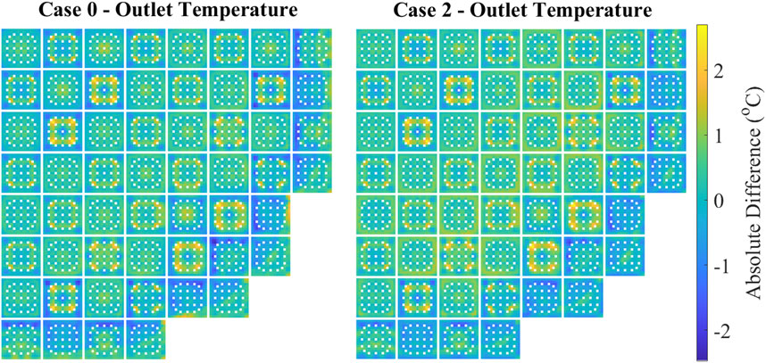
Figure 8. Absolute difference of the pinwise coolant temperature at the outlet of the core as calculated by nTRACER/CTF vs. nTRACER/ML for Cases 0 and 2.

The maps of the outlet coolant temperature difference at the pin level are indicative of the performance of the ML module when providing T/H feedback. As explained by Papadionysiou et al. (2025a), the maximum discrepancies of ML-CTF-Cool appear at the top of the active core. The discrepancy patterns observed in Figure 8 are consistent with the conclusions of the verification study for ML-CTF-Cool conducted by Papadionysiou et al. (2025a). The biggest differences appear in areas with strong power gradients, specifically the edges of assemblies with neighbors of lower enrichment and where several Pyrex rods are clustered together. However, the maximum difference does not exceed 2.63 °C, even in Case 2, where the water liner is introduced in the CTF model. More importantly, the RMSE of the pin coolant outlet temperature is 0.60% for Case 0 and 0.62% for Case 2, while the RMSE of the pin coolant temperature difference over all axial layers does not exceed 0.65% for all cases. This indicates good agreement between nTRACER/CTF and nTRACER/ML. Figure 8 also shows that the radial tilt of the pin power difference over the core and the concave pin power difference profiles inside assemblies are related to the coolant temperature discrepancies. Except for the outer assemblies next to the reflector, ML tends to underestimate coolant temperature closer to the reflector, while this effect is less pronounced toward the core center, especially in Case 2. Though the resulting tilt is minor, it contributes to the weak power tilt seen in Figure 6. Within assemblies, ML overestimates coolant temperature at the edges and underestimates it in the center, leading to a concave pin power difference, lower at the edges and higher at the center, superimposed on the radial power tilt.

The performance of the ML module is further evaluated in terms of its accuracy in predicting fuel temperature. Table 5 presents the maximum absolute differences and RMSEs for Cases 0–2 for the coolant temperature and the fuel temperature, at the centerline, surface, and average, over all axial layers. It is important to note that the errors from ML-CTF-Cool propagate into the predictions of ML-CTF-Fuel, meaning the accuracy observed by Papadionysiou et al. (2025b) is not expected in this work. Table 5 clearly shows that the presence of spacer grids significantly impacts the accuracy of ML-CTF-Fuel. In Case 1, the maximum discrepancies for the centerline, surface, and average fuel pin temperatures are approximately double those in Case 0. Specifically, the maximum absolute differences reach 33.25 °C, 9.76 °C, and 29.21 °C for centerline, surface, and average temperatures, respectively. The RMSEs of the centerline and average temperatures also double in Case 1, reaching 5.59 °C and 5.94 °C, while the RMSE for surface temperature increases from the 1.50 °C in Case 0 °C to 1.87 °C in Case 1. The discrepancies observed in Case 2 for fuel temperature are of a similar magnitude to those in Case 1. In contrast, the discrepancies observed in the coolant remain unchanged between Cases 0 and 1, with a slight increase in Case 2. This proves that the discrepancies of Case 1 in terms of fuel temperature cannot be directly correlated to the predictions of ML-CF-Cool but rather to the presence of spacer grids. A second key observation from Table 5 is that the discrepancies in average fuel pin temperature are larger than those for the centerline and surface temperatures in all cases in terms of RMSE. To further analyze these effects, as well as the impact of spacer grids on ML-CTF-Fuel predictions, Figure 9 presents the axial profiles of centerline, surface, and average fuel temperatures as calculated by nTRACER/CTF and nTRACER/ML for Cases 0 and 2, along with their absolute differences. $\left[{Temp}_{nTRACER/CTF}-{Temp}_{nTRACER/ML}\right]$.

Table 5

Table 5. Maximum absolute difference and RMSE over all axial layers for the centerline, surface, and average fuel pin temperatures and coolant pin temperatures of nTRACER/CTF vs. nTRACER/ML for all test cases.

Figure 9

Figure 9. Axial profile of the centerline (left), surface (middle), and average (right) fuel temperatures as predicted by both solvers, together with their absolute differences for Cases 0 (upper plots) and 2 (lower plots).

Figure 9 supports the observations from Table 5, highlighting the impact of spacer grids on fuel temperature predictions. Comparing Case 2 with Case 0 shows that the absolute difference profiles are strongly influenced by the presence of spacer grids, with nTRACER/ML overestimating fuel temperature at the axial nodes where spacer grids are modeled. This can be partly attributed to the pressure loss caused by spacer grids, which is not accounted for in the training of ML-CTF-Fuel. However, the main cause for discrepancies is probably the mismatched axial profiles of the ML models and nTRACER, leading to partial averaging of local properties. In Case 0, aside from the axial nodes at the core edges, nTRACER/ML tends to underestimate the centerline and surface temperatures while overestimating the average fuel temperature. This suggests that the quasi-parabolic profile used for fuel temperature reconstruction, defined with an exponent of p = 1.78 based on a sensitivity study (see Section 2.3.2), contributes to the discrepancies observed in the average fuel temperature, specifically for the HFP case. This is not expected to be a source of discrepancy for the cycle analysis. The conductivity changes with BU; thus, a single value of the exponent p for the whole cycle cannot be optimal at all conditions of exposure. In any case, the resulting discrepancies are not significant.

Despite these discrepancies, nTRACER/ML demonstrates strong overall agreement with nTRACER/CTF, as seen in the comparisons of power and coolant temperature values, as well as the RMSE of the absolute difference in fuel temperature.

5.2 First cycle

The first cycle of TVA WB1 described in the benchmark specification (Exercise 3) uses the fresh fuel loading pattern shown in Figure 3. As can be observed in Figure 4, the detailed power history of the cycle is simplified by the benchmark team with larger BU steps of averaged operating conditions to facilitate the simulation of the full cycle by novel codes with high computational costs. nTRACER/CTF has been verified with VERA for the whole first cycle of TVA WB1 (Kwon et al., 2025). At the current stage of development, the local BU is not considered in the T/H calculation by nTRACER/CTF. On the other hand, as mentioned in Section 2.3.2, ML-CTF-Fuel is trained with CTF calculations that take into account the effect of local BU on the fuel properties. In order to provide an equivalent reference solution, three specific BU steps are selected from the simplified power history for which the nTRACER/CTF calculation is repeated, considering the local BU in the T/H calculations. It must be pointed out that nTRACER/CTF is not modified in this work to consider BU in the T/H calculation. The local BU for the specific BU step, which is calculated by Kwon et al. (2025), is set a priori in the relevant CTF input. To ensure consistency in the comparison, the nTRACER/ML calculations are also performed for the three selected BU steps with the same local BU distribution as predicted by nTRACER/CTF in Kwon et al. (2025).

The first BU step for comparison is selected at the beginning of the cycle (BOC), once the core power reaches 100% at 78 effective full power days (EFPDs). The two other BU steps are selected at the middle of the cycle (MOC) and at the end of the cycle (EOC) at 221.1 EFPDs and 392.3 EFPDs, respectively. It must be pointed out that there were some convergence issues in the nTRACER/ML calculation at the EOC, so an initial guess for the local power profile is applied. This will be discussed further in this section. Figure 10 presents the absolute difference of the axially averaged pin power of nTRACER/CTF vs. nTRACER/ML, [${power}_{nTRACER/CTF}-{power}_{nTRACER/ML}$], for the steps at BOC and EOC. The results for the MOC are excluded because the discrepancies are similar to those of the BOC and EOC. Figure 11 presents the normalized axial power profile as it is calculated from both core solvers for the three BU steps, together with the relevant absolute difference. Table 6 summarizes the maximum absolute difference and RMSE of the 3D assembly power, the axially averaged pin power, the axial power profile, and the critical boron concentration (CBC) as calculated by nTRACER/CTF and nTRACER/ML for the three BU steps.

Figure 10

Figure 10. Absolute difference of the axially averaged pin power of nTRACER/CTF vs. nTRACER/ML at 78 EFPDs and 392.3 EFPDs.

Figure 11

Figure 11. Normalized axial power profile calculated by nTRACER/CTF and nTRACER/ML together with their absolute difference at 78 EFPDs (left), 221.1 EFPDs (middle), and 392.3 EFPDs (right).

Table 6

Table 6. Maximum absolute difference and RMSE of the nTRACER/CTF solution vs. nTRACER/ML for the 3D assembly power, axially averaged pin power (2D), and axial power profile (1D) for 78 EFPDs, 221.1 EFPDs, and 392.3 EFPDs.

The difference of the calculated CBC remains below 4 ppm at the BOC, almost identical to the HFP value (see Table 4), and decreases with exposure. Considering Figures 6, 10; Tables 3 and 5, it is apparent that the discrepancies in terms of axially averaged pin power between nTRACER/CTF and nTRACER/ML are similar to what is observed for the HFP case throughout the cycle. The maximum pin power difference does not exceed 0.33%, and the RMSE does not exceed 0.12%, with the levels of discrepancy at the MOC being even lower than those observed for BOC and EOC. The patterns of discrepancy are also very similar to the ones presented for HFP. However, this is not the case for the axial power profile. At the BOC, the axial profile of discrepancy is similar to the HFP case, both in shape and value, with the maximum reaching 0.62% and an RMSE of 0.30%. As exposure increases and the power profile is becoming flatter, nTRACER/ML increasingly underestimates the power at the bottom half of the core and overestimates it at the top half, reaching a maximum of 3.33% at the EOC. The same discrepancies are apparent in the 3D assembly power comparison, with the maximum reaching 4.13 at the EOC with an RMSE of 2.27%. It must be pointed out that, despite the higher discrepancies, the predictions of nTRACER/ML can be considered sufficiently accurate compared to nTRACER/CTF, especially when considering that the intended use of nTRACER/ML is as a lower-fidelity solver. The maximum local pin power difference is less than 4.3%. At the same time, the maximum discrepancies of the axial power profile remain at the same level with the respective quantities of the nTRACER/CTF vs. VERA verification (Kwon et al., 2025). In Kwon et al. (2025), the maximum difference in the axial power profile is 4.09% and the RMSE is 2.34%. Therefore, while these levels of discrepancy are relatively high, they are not uncommon in comparisons of multi-physics core simulations developed using tools based on different methodologies. Further insight can be gained by comparing the coolant and fuel temperature distributions.

Table 7 presents the maximum absolute differences and RMSEs of the coolant temperatures and the fuel temperatures, at the centerline, surface, and average, over all axial layers, $\left[{Temp}_{nTRACER/CTF}-{Temp}_{nTRACER/ML}\right]$, for the BOC, MOC, and EOC. Figure 12 presents the axial profiles of the coolant temperature as calculated by nTRACER/CTF and nTRACER/ML for the BOC, MOC, and EOC, along with the absolute difference. Several observations can be made when comparing Table 7 and Table 5. First, the discrepancies of the coolant temperature are becoming less pronounced with exposure. Already at the BOC, the maximum discrepancy is less than what is observed for the HFP case. At the EOC, it drops to 1.68 °C from the corresponding 2.63 °C value for HFP. A similar trend is observed for the RMSE, dropping from 0.65 °C to 0.53 °C. The radial patterns of discrepancy for the three BU steps are the same as those presented in Figure 8; however, they are less pronounced. It must be pointed out that the decrease in discrepancies with exposure in the predictions of ML-CTF-Cool is expected because the local power distribution becomes more homogeneous. The study conducted by Papadionysiou et al. (2025a) showed that ML-CTF-Cool performs better for less heterogeneous power profiles both radially and axially. This is also apparent in Figure 12, which compares the axial coolant temperature profiles. At the same time, Figure 12 shows that at the EOC, the temperature difference partly follows the sigmoid profile of the axial power difference. This is more apparent at the top of the core, where nTRACER/ML underestimates the coolant temperature more than it does for the BOC and MOC. In any case, nTRACER/ML presents very good agreement with nTRACER/CTF in terms of coolant temperature for all BU steps.

Table 7

Table 7. Maximum absolute differences and RMSEs averaged over all axial layers for the centerline, surface, and average fuel pin temperature and coolant pin temperature of nTRACER/CTF vs. nTRACER/ML at 78 EFPDs, 221.1 EFPDs, and 392.3 EFPDs.

Figure 12

Figure 12. Axial profile of the coolant temperature predicted by both solvers together with the absolute difference for 78 EFPDs (left), 221.1 EFPDs (middle), and 392.3 EFPDs (right).

Despite the decreased difference in terms of coolant temperature as BU increases, the predictions of ML-CTF-Fuel present some interesting trends. The surface fuel temperature at 78 EFPDs presents higher discrepancies than those observed for the HFP case in terms of RMS, which increases from 1.89% to 3.07%. The maximum difference is also increased but by less than 1 °C. The possible cause is gap closure, which, as presented by Papadionysiou et al. (2025b), can be a source of discrepancy in the predictions of ML-CTF-Fuel, especially for surface temperature. As BU increases, the discrepancies also decrease, as gap closure is no longer an issue, and the coolant temperature predictions improve. Nonetheless, the RMSE remains higher than what is observed for the HFP case at 2.43% for the EOC. The discrepancies of the centerline temperature also increase in terms of RMSE at 78 EFPDs compared to the HFP case, from 5.55 °C to 6.48 °C, probably also due to gap closure. On the other hand, the biggest discrepancies are observed at the EOC, with the maximum difference reaching 36.24 °C and the RMSE reaching 8.30 °C. The average temperature presents overall better agreement for the BU steps than for the HFP, which is expected because the exponential parameter p = 1.78 of the fuel reconstruction profile is optimized for cycle analysis. The level of discrepancies for the fuel temperature, even though higher than that observed for the HFP case, remains within acceptable limits in terms of safety. With regard to neutronics, calculating the Doppler temperature difference for the pin of maximum discrepancy, (4/9 ∙ Tcent + 5/9∙ Tsurf) [Rowlands correlation], and considering that 1 °C of difference in the Doppler temperature results is approximately 3 pcm of the discrepancy (Mathieu Hursin, personal communication, 30 October 2024), the local discrepancy amounts to less than 70 pcm, which is well within target accuracy (Tractabel, 2021). For depletion calculations, fuel temperatures that can lead to safety issues [e.g., fuel melting, strong pellet-cladding mechanical interaction (PCMI)] are higher than the observed discrepancies. The FRAPCON validation studies indicate that a 4% error is expected on the average centerline fuel temperature (Geelhood and Luscher, 2015). The maximum discrepancy observed on the centerline at 392.3 EFPDs corresponds to ∼4.5% of the average centerline temperature, and the RMSE corresponds to ∼1%, indicating that the discrepancies are well within acceptable limits. To gain a deeper understanding of the evolution of the fuel temperature discrepancies with exposure, Figure 13 presents the axial profiles of centerline, surface, and average fuel temperatures calculated by nTRACER/CTF and nTRACER/ML for the three BU steps, along with their absolute differences. $\left[{Temp}_{nTRACER/CTF}-{Temp}_{nTRACER/ML}\right]$.

Figure 13

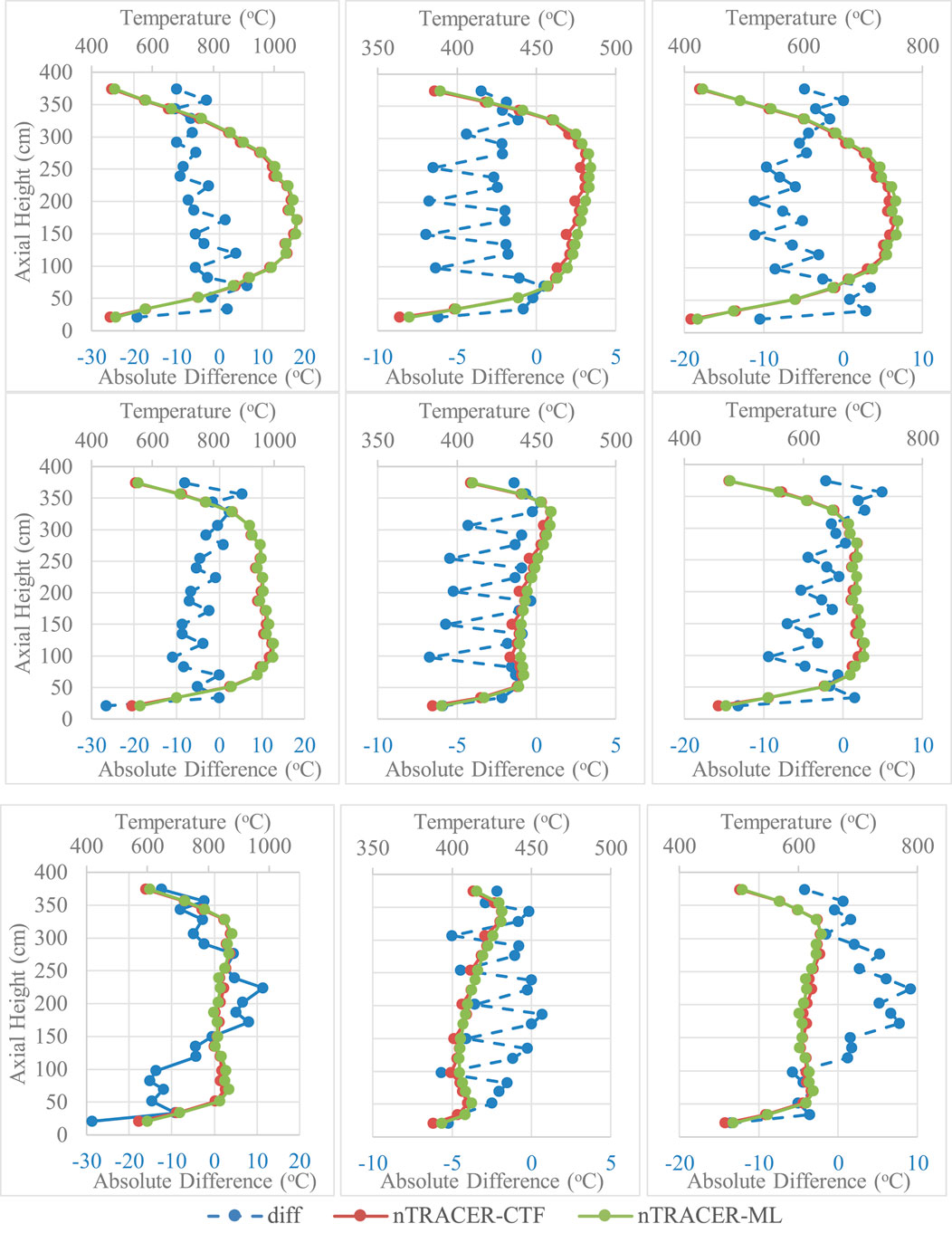
Figure 13. Axial profile of the centerline (left), surface (middle), and average (right) fuel temperatures predicted by both solvers together with their absolute difference for 78 EFPDs (upper plots), 221.1 EFPDs (middle plots), and 392.3 EFPDs (lower plots).

As expected, the centerline temperature profile follows the power profile, while the surface (especially after the gap closure) follows the coolant temperature profile. At the BOC, the shapes of the axial profiles of the centerline, surface, and average temperature are very similar to the respective diagrams of the HFP case. However, as BU increases, the profiles present changes that are significant in the case of the centerline and average temperature. At 392.3 EFPDs, the distribution of the axial temperature differences presents a peak at the mid-height of the core and a dip at the bottom of the core, which are not observed for 221.1 EFPDs or 78 EFPDs. The same pattern is apparent on the axial average temperature profile, which follows the evolution of the centerline temperature because the surface temperature difference does not present strong discrepancies. To illustrate this trend, the radial distribution of the centerline temperature difference is presented in Figure 14, at a height of 69.22 cm from the bottom of the core, where the maximum discrepancy in the axial power profile appears. At 78 EFPDs, nTRACER/ML underestimates the centerline temperature for all pins by a maximum of 10 °C, more strongly in the center and less toward the reflector region. At 221.1 EFPDs, the temperature difference ranges between ±2.5 °C, and at 392.3 EFPDs, nTRACER/ML overestimates the temperature on all pins with a maximum of 17 °C.

Figure 14

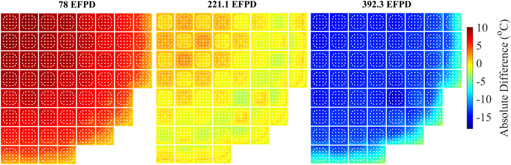
Figure 14. Radial distribution of the absolute differences for the centerline temperature at 69.22 cm from the bottom of the core for 78 EFPDs, 221.1 EFPDs, and 392.3 EFPDs.

A possible cause for the increased discrepancies as BU increases is the range of applicability of ML-CTF-Fuel. However, at this point in the study, it is not clear to the authors if the higher discrepancies in the power profile as BU increases are the cause or consequence of the shift in the fuel temperature difference observed at different BU steps. Several studies were conducted to identify the cause of discrepancies, such as convergence studies at the different BU points. Nonetheless, a more detailed analysis involving decoupling the different solvers and testing their range of applicability beyond the operational limits of TVA WB1 is necessary. This is the next stage of this study, together with the convergence issues of nTRACER/ML for higher BU. In any case, this work presents an initial effort to couple the solvers. The presented discrepancies are not negligible but, as was already discussed, remain within acceptable limits for comparison of multi-physics core solvers.

The convergence issue at 392.3 EFPDs, which made the use of an initial guess in the power profile necessary, was caused by the local power distribution calculated during the first CMFD iteration of nTRACER. Local power calculated by the first CMFD iteration can take progressively higher values as BU increases, which exceed by far the power levels of normal operation and the range of applicability of ML-CTF-Fuel. This results in the ML model significantly overpredicting the local fuel temperature, due to the necessary extrapolation. For example, the maximum RMSE of an axial layer is 18 °C, and the maximum discrepancy is 61 °C in terms of centerline temperature. The same phenomenon occurs for ML-CTF-Cool; however, the predictions do not reach significantly higher discrepancies than those observed at the end of the calculation (maximum RMSE 1.2 °C vs. 0.8 °C and maximum discrepancy 2.45 °C). This is expected because ML-CTF-Cool is more robust and has a larger verified range of applicability than ML-CTF-Fuel (Papadionysiou et al., 2025a; Papadionysiou et al., 2025b). Due to the significant overprediction of fuel temperature, the power predicted by nTRACER is also decreased significantly locally, resulting in an underprediction of the fuel temperature at the second T/H iteration. Thus, the power profile oscillates, making it difficult to converge. The same behavior is observed in the 221.1 EFPDs nTRACER/ML calculation; however, it is not so pronounced. As the calculation progresses and the local power converges, the local power distribution remains within the expected limits of normal operation and the range of applicability of ML-CTF-Fuel. A possible solution would be the extension of the application range of ML-CTF-Fuel and possibly ML-CTF-Cool. However, a more efficient measure would be the application of relaxation factors on the power distribution used by the ML models and the T/H feedback provided to nTRACER.

Despite the observed discrepancies, nTRACER/ML presents good enough agreement with nTRACER/CTF, in terms of neutronic and T/H parameters, and can be used as a low-fidelity solver for high-resolution calculations even at the current stage of development.

5.3 Computational cost

As mentioned by Papadionysiou et al. (2025a) and Papadionysiou et al. (2025b), the CTF is significantly more computationally expensive than the ML models. Table 8 presents the computational cost of CTF and the ML models in the HFP calculation, together with the calculations at 78 EFPDs and 221.1 EFPDs. The calculation for the third BU step is not included because an initial power profile was applied to nTRACER/ML to accelerate convergence. The memory cost is not included in Table 8 because this is defined by nTRACER.

Table 8

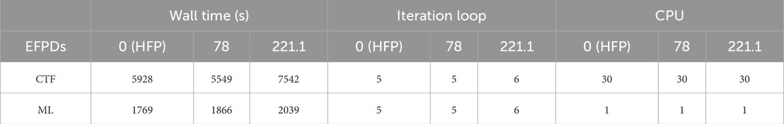
Table 8. Computational costs of CTF and ML for the HFP case and the BU step calculations at 78 EFPDs and 221.1 EFPDs.

As expected, the computational cost of the ML models is significantly less than that of the CTF. Despite the fact that currently no parallelization is used in the Python wrapper presented in Figure 2, the T/H feedback provided by the ML models is 3–4 times faster than CTF and requires only 1% of the CTF CPU time. That means that the acceleration is actually even larger than what we see by comparing only the wall time. It is also important to note that the ML models require the same number of iterations to converge the T/H solution as CTF with the same convergence criterion. It must be pointed out that the wall time tallied for the ML models also includes the processing of all necessary files by nTRACER (listed in Figure 2), which is ∼11 min. There is a large room for improvement in the coupling scheme between nTRACER and the ML models. First, the ML models can be parallelized. In addition, the data exchange could be performed more efficiently and not through external files. It is expected that if nTRACER is coupled with the ML models as tightly as it is with CTF and the ML models are parallelized, the T/H feedback will be 10 or more times faster than CTF (Papadionysiou et al., 2025a). This is part of the future work for this study.

6 Conclusion and future work

LRT has developed a high-resolution multi-physics simulation tool for Cartesian PWRs, using the latest versions of nTRACER and CTF for cycle analysis. In parallel, and to provide a lower-cost alternative to nTRACER/CTF, LRT—together with NCSU—is developing a second high-resolution multi-physics core solver. This alternative approach couples nTRACER with two ML models designed to predict coolant and fuel properties, respectively. These ML models have been independently verified against standalone CTF simulations across the full range of operating conditions described in the three depletion cycles of the TVA WB1 benchmark. The present work focuses on verifying nTRACER/ML with nTRACER/CTF within the TVA WB1 framework. To the authors’ knowledge, this represents the first attempt to use ML-based models to provide high-resolution T/H feedback to a sub-pin neutronic solver for full-core cycle analysis. The TVA WB1 HFP case is used to verify nTRACER/ML against nTRACER/CTF and to assess the impact of specific ML model approximations on solution accuracy. Finally, the results of nTRACER/ML for the first depletion cycle of TVA WB1 are presented, with comparisons at selected BU points to nTRACER/CTF results, including an evaluation of the computational performance of the respective T/H solvers.

Despite approximations in the ML model training, such as excluding spacer grids and the water liner, nTRACER/ML shows strong agreement with nTRACER/CTF for the HFP case in both global and local quantities. The CBC difference is ∼4 ppm. Introducing spacer grids and the water liner increases discrepancies slightly, with maximum deviations of 1.01% in assembly power and 0.72% in axial power, both within acceptable limits. The RMSEs for both quantities stay below 0.40%. The axially averaged pin power agrees closely, with a maximum absolute difference of 0.31% and an RMSE of ∼0.10%. Coolant temperature difference maps confirm trends observed in the ML-CTF-Cool verification study (Papadionysiou et al., 2025a). The maximum difference remains at 2.63 °C and the RMSE at 0.65%, even when compared with a CTF calculation including the water liner. On the other hand, ML-CTF-Fuel predictions are significantly affected by spacer grids, with fuel temperature discrepancies nearly doubling: up to 32.96 °C (centerline), 9.67 °C (surface), and 28.89 °C (average), and RMSEs of 5.55 °C, 1.89 °C, and 5.84 °C, respectively. In contrast, coolant discrepancies remain stable, with only a slight increase when including the water liner. These errors partly stem from axial profile mismatches between ML models and nTRACER, especially when spacer grids are present. Despite these discrepancies, nTRACER/ML demonstrates strong overall agreement with nTRACER/CTF in terms of local power and temperature.

Three BU steps (78 EFPDs, 221.1 EFPDs, and 392.3 EFPDs) from the first TVA WB1 cycle were selected, using nTRACER/CTF with local BU-dependent T/H feedback as the reference for nTRACER/ML. The CBC difference stays under 4 ppm at BOC and decreases with exposure. Axially averaged pin power discrepancies remain similar to the HFP case, but assembly and axial power profiles deviate more with exposure. As the axial power profile flattens, nTRACER/ML increasingly underestimates the power at the bottom and overestimates it at the top of the core, reaching a 3.33% axial power discrepancy and 4.13% in 3D assembly power at the EOC (RMSE: 2.27%). Coolant temperature discrepancies decrease with exposure, with a maximum of 1.68 °C and an RMSE of 0.53 °C at EOC, consistently with the ML-CTF-Cool verification study (Papadionysiou et al., 2025a). In contrast, fuel temperature discrepancies increase. Surface temperature shows the largest errors at 78 EFPDs (RMSE: 3.07%), likely due to gap closure, while centerline temperature peaks at EOC (36.24 °C, RMSE: 8.30 °C). Average temperature presents better agreement than the HFP case because the exponential parameter (p = 1.78) of the fuel temperature profile is cycle optimized. Identifying the possible causes for the increase in discrepancies with BU and applying some relaxation factors in the coupling scheme in the hope of improvement is the next step of this work.

Despite these limitations, nTRACER/ML achieves sufficient agreement with nTRACER/CTF across neutronic and T/H metrics, making it a viable low-fidelity alternative for high-resolution simulations, especially considering that it is 3–4 times faster than CTF and requires only 1% of the CPU time. In the future, this study will focus on improving the ML models and increasing their range of applicability. In addition, relaxation parameters will be introduced in the power distribution fed to the ML models and on their T/H feedback. Finally, the coupling scheme will become more efficient by minimizing the time necessary for the data exchange and parallelizing the ML models. The improved nTRACER/ML will be verified for every BU step of the simplified curve of the TVA WB1 first cycle, with a solution of equivalent capabilities (taking into account BU for calculation of material properties), and the two subsequent cycles described in the benchmark.

Data availability statement

The datasets presented in this article are not readily available because that are generated with codes requiring licensing. Requests to access the datasets should be directed to aGFraW0uZmVycm91a2hpQHBzaS5jaA==.

Author contributions

MP: Conceptualization, Data curation, Formal Analysis, Investigation, Methodology, Software, Validation, Visualization, Writing – original draft, Writing – review and editing. GD: Conceptualization, Data curation, Investigation, Methodology, Validation, Visualization, Writing – review and editing. MA: Funding acquisition, Project administration, Resources, Software, Supervision, Writing – review and editing. HF: Funding acquisition, Project administration, Resources, Supervision, Writing – review and editing. KI: Funding acquisition, Project administration, Resources, Software, Supervision, Writing – review and editing.

Funding

The authors declare that financial support was received for the research and/or publication of this article. This work was partly funded by the Swiss Nuclear Safety Inspectorate ENSI (CTR00943) and was conducted within the framework of the STARS program (http://www.psi.ch/stars). It has also been supported by the Consortium for Nuclear Power (CNP) at North Carolina State University, USA.

Conflict of interest

The authors declare that the research was conducted in the absence of any commercial or financial relationships that could be construed as a potential conflict of interest.

Generative AI statement

The authors declare that Generative AI was used in the creation of this manuscript. During the preparation of this work, the authors used ChatGPT in order to improve the syntax and grammar of the text in specific sections. After using this tool, the authors reviewed and edited the content as needed and take full responsibility for the content of the publication.

Any alternative text (alt text) provided alongside figures in this article has been generated by Frontiers with the support of artificial intelligence and reasonable efforts have been made to ensure accuracy, including review by the authors wherever possible. If you identify any issues, please contact us.

Publisher’s note

All claims expressed in this article are solely those of the authors and do not necessarily represent those of their affiliated organizations, or those of the publisher, the editors and the reviewers. Any product that may be evaluated in this article, or claim that may be made by its manufacturer, is not guaranteed or endorsed by the publisher.

References

Agarwal, V. (2022). “Technical basis for advanced artificial intelligence and machine learning adoption,” in Nuclear power plants United States: US Department of Energy. doi:10.2172/1889877

CrossRef Full Text | Google Scholar

Albagami, T., Rouxelin, P., Abarca, A., Holler, D., Moloko, L., and Avramova, M. (2022). “TVA watts Bar unit 1 multi-physics Multi- cycle depletion benchmark specifications and support data.

Google Scholar

Avramova, M., Abarca, A., Hou, J., and Ivanov, K. (2021). Innovations in multi-physics methods development, validation, and uncertainty quantification. J. Nucl. Eng. 2 (1), 44–56. doi:10.3390/jne2010005

CrossRef Full Text | Google Scholar

Choi, N., and Joo, H. G. (2020). Stability enhancement of planar transport solution based whole-core calculation employing augmented axial method of characteristics. Ann. Nucl. Energy 143, 107440. doi:10.1016/j.anucene.2020.107440

CrossRef Full Text | Google Scholar

Clifford, I., Pecchia, M., Mukin, R., Cozzo, C., Ferroukhi, H., and Gorzel, A. (2019). Studies on the effects of local power peaking on heat transfer under dryout conditions in BWRs. Ann. Nucl. Energy 130, 440–451. doi:10.1016/j.anucene.2019.03.017

CrossRef Full Text | Google Scholar

Delipei, G. K., Rouxelin, P., and Hou, J. (2023). Reactor Core loading pattern optimization with reinforcement learning. Int. Conf. Math. Comput. Methods Appl. Nucl. Sci. Eng. (M&C 2023).

Google Scholar

D’Auria, F. (2019). Best Estimate Plus Uncertainty (BEPU): status and perspectives. Nucl. Eng. Des. 352 (November 2018), 110190. doi:10.1016/j.nucengdes.2019.110190

CrossRef Full Text | Google Scholar

García, M., Bilodid, Y., Basualdo Perello, J., Tuominen, R., Gommlich, A., Leppänen, J., et al. (2021). Validation of Serpent-SUBCHANFLOW-TRANSURANUS pin-by-pin burnup calculations using experimental data from a Pre-Konvoi PWR reactor. Nucl. Eng. Des. 379 (March), 111173. doi:10.1016/j.nucengdes.2021.111173

CrossRef Full Text | Google Scholar

Geelhood, K. J., and Luscher, W. G. (2015). “FRAPCON-4.0: integral assessment,” vol. 2, no. September, p. 408.

PubMed Abstract | Google Scholar

Goodfellow, I., Bengio, Y., and Courville, A. (2017). Deep learning. MIT Press 521 (7553), 785. doi:10.1016/B978-0-12-391420-0.09987-X

CrossRef Full Text | Google Scholar

Hastie, T., Tibshirani, R., and Friedman, J. (2009). The elements of statistical learning. Math. Intell. 27(2), 83–85. Available online at: http://www.springerlink.com/index/D7X7KX6772HQ2135.pdf.

Google Scholar

He, D., and Walters, W. J. (2020). Development of RAPID transport calculation with heterogeneous temperature distribution. Ann. Nucl. Energy 148, 107685. doi:10.1016/j.anucene.2020.107685

CrossRef Full Text | Google Scholar

IAEA (2017). Opportunities for cogeneration with nucelar energy.

Google Scholar

Kelley, B. W. (2015). An investigation of 2D/1D approximations to the 3D Boltzmann transport equation. Michigan Univ. PhD Thesis, 1–137.

Google Scholar

Kochunas, B., Collins, B., Stimpson, S., Salko, R., Jabaay, D., Graham, A., et al. (2017). VERA core simulator methodology for pressurized water reactor cycle depletion. Nucl. Sci. Eng. 185 (1), 217–231. doi:10.13182/NSE16-39

CrossRef Full Text | Google Scholar

Kwon, S. J., Papadionysiou, M., Jung, Y. S., Rouxelin, P., Vasiliev, A., Ferroukhi, H., et al. (2025). Verification of the nTRACER/CTF code System for full core high resolution cycle analysis with the OECD/NEA TVA watts bar unit 1 benchmark. Ann. Nucl. Energy. doi:10.1016/j.anucene.2025.111532 PhD Thesis.

CrossRef Full Text | Google Scholar

Papadionysiou, M., Kim, S., Hursin, M., Vasiliev, A., Ferroukhi, H., Pautz, A., et al. (2022). “Coupling of COBRA-TF to nTRACER for full core high-fidelity analysis of VVERs,” in International conference on physics of reactors: transition to a scalable nuclear future (PHYSOR), 170–177. doi:10.1051/epjconf/202124702008

CrossRef Full Text | Google Scholar

Papadionysiou, M., Albagami, T., Delipei, G., Avramova, M., Vasiliev, A., Ferroukhi, H., et al. (2024). Multi-physics Sub-pin resolution Analysis of a PWR core with nTRACER/CTF for the OECD/NEA TVA Watts Bar 1 benchmark. Int. Conf. Phys. React., 1968–1977. doi:10.13182/physor24-43543

CrossRef Full Text | Google Scholar

Papadionysiou, M. (2022). Multi-physics modeling of VVERs with high fidelity high-resolution codes. Lausanne: Swiss Federal Institute of Technology.

Google Scholar

Papadionysiou, M., Seongchan, K., Hursin, M., Vasiliev, A., Pautz, A., and Joo, H. G. (2022). Validation of the novel core solver nTRACER/COBRA-TF for Full core High Fidelity Cycle Analysis of VVERs. Nucl. Eng. Des. 398 (November), 111946.

Google Scholar

Papadionysiou, M., Delipei, G., Avramova, M., Ferroukhi, H., and Ivanov, K. (2025a). High-resolution predictions of the coolant properties for the 3D PWR core with artificial neural networks based on CTF. Nucl. Energy Des. 442, 814–823. doi:10.1016/j.nucengdes.2025.114261

CrossRef Full Text | Google Scholar

Papadionysiou, M., Delipei, G., Avramova, M., and Ferroukhi, H. (2025b). “High-resolution predictions of the fuel and cladding temperatures for the 3D PWR core with artificial neural networks trained on CTF,” in M&C 2025 - International Conference on Mathematics and Computational Methods Applied to Nuclear Science and Engineering. under review.

Google Scholar

Ramos, A., Carrasco, A., Fontanet, J., Herranz, L., Ramos, D., Díaz, M., et al. (2024). Artificial intelligence and machine learning applications in the Spanish nuclear field. Nucl. Eng. Des. 417 (December 2023), 112842. doi:10.1016/j.nucengdes.2023.112842

CrossRef Full Text | Google Scholar

Ryu, M., Jung, Y. S., Cho, H. H., and Joo, H. G. (2015). Solution of the BEAVRS benchmark using the nTRACER direct whole core calculation code. J. Nucl. Sci. Technol. 52 (7–8), 961–969. doi:10.1080/00223131.2015.1038664

CrossRef Full Text | Google Scholar

Salko, R. K., and Avramova, M. N. (2015). “COBRA-TF subchannel code (CTF) theory manual”.

Google Scholar

Song, J. H., and Kim, S. J. (2024). A machine learning informed prediction of severe accident progressions in nuclear power plants. Nucl. Eng. Technol. 56 (6), 2266–2273. doi:10.1016/j.net.2024.01.035

CrossRef Full Text | Google Scholar

Spasov, I., Mitkov, S., Kolev, N., Sanchez-Cervera, S., Garcia-Herranz, N., Sabater, A., et al. (2017). Best-estimate simulation of a VVER MSLB core transient using the NURESIM platform codes. Nucl. Eng. Des. 321, 26–37. doi:10.1016/j.nucengdes.2017.03.032

CrossRef Full Text | Google Scholar

Tong, L. S., and Weisman, J. (1979). Thermal analysis of pressurized water reactors. American Nuclear Society. doi:10.1177/002072097000800329

CrossRef Full Text | Google Scholar

Tractabel (2021). WPEC Subgroup 46 Activity on ‘Target Accuracy Requirements (TAR)’ Core physics validation.

Google Scholar