Small signal stability prediction and correction control algorithm for wind power systems based on LightGBM

With the increasing penetration of wind power in electrical power systems, its impact on small signal stability has become increasingly significant. The volatility and uncertainty introduced by wind power integration pose new challenges to power system stability analysis and control. To accurately predict and correct the small signal stability of wind power systems, this paper proposes a prediction and correction method based on the Light Gradient Boosting Machine (LightGBM) algorithm. The LightGBM model offers high computational efficiency and low memory consumption, enabling large-scale data processing and automatic handling of missing values, thereby accurately extracting grid characteristics. To verify the reliability of the proposed method, Gaussian white noise with three different signal-to-noise ratios is introduced to evaluate the model’s performance and robustness. Case studies are conducted using a 3-machine 9-bus system and a 10-machine 39-bus system, in which certain conventional generators are replaced with aggregated wind farms. By applying the LightGBM model to predict the system’s minimum damping ratio and constructing a correction optimization model based on damping ratio sensitivity, unstable operating states are effectively adjusted. Simulation results demonstrate that the proposed method achieves high prediction accuracy and rapid correction response, confirming its feasibility and effectiveness in small signal stability analysis and control of wind-integrated power systems.

1 Introduction

With the continuous progress of science and technology and the sustained development of the economy, environmental pollution and excessive consumption of resources have increasingly become the focus of social attention. In this context, new energy generation technologies mainly based on wind power are rapidly developing. Compared to traditional energy generation methods, wind power generation does not produce carbon emissions during operation, is sustainable, and power generation facilities can be built on land or deployed in the ocean. As an important component of the future power grid, wind power generation has received high attention from the country.

However, it is difficult to avoid small interference problems during the operation of the power system. Once the system becomes unstable due to small interference, it will seriously affect its normal operation. Wind turbines have characteristics such as randomness, volatility, and intermittency. When they are integrated into a large power grid, they can have an impact on the small signal stability of the power system. Therefore, effective monitoring and adjustment of power systems containing wind power generation are crucial for maintaining the stable operation of the power system.

Common methods for analyzing small signal stability in power systems include damping torque method (Yanfeng et al., 2020; Gibbard et al., 2015) and eigenvalue analysis method. The derivation of damping torque analysis method is complex and commonly used to analyze single machine infinite bus systems. Therefore, the eigenvalue analysis method is commonly used for multi machine power systems (Jiang et al., 2021). The eigenvalue calculation method is based on the Lyapunov linearization method, which transforms nonlinear problems into linear problems and obtains the state matrix of linear differential algebraic equations based on eigenvalues to determine the stability of the system. Traditional eigenvalue calculation methods include QR (QR Algorithm) method, Arnoldi, and Jacobi Davidson. These methods require a large amount of computation and are difficult to reflect the real-time operating status of the power system.

Frequency domain analysis is a fundamental tool for small signal stability analysis of multi machine power systems. The advantage of this method is that it can handle any type of generator model; It can directly obtain frequency domain data and has good computational efficiency. However, for large-scale power systems, this method still requires a significant amount of computation and cannot meet the requirements of fast calculation (Zeng and Jun, 2020).

In recent years, the research on nonlinear theory has achieved extensive development. For instance, bifurcation theory and chaos theory have been gradually introduced into the study of small-signal stability analysis in power systems. A Hopf Bifurcation Point (HB) refers to an equilibrium point where a pair of conjugate eigenvalues crosses the imaginary axis from the left half-plane to the right half-plane in the complex plane as system parameters change. The imaginary axis in the complex plane, as described by this concept, serves as the boundary condition for the small-signal stability of a system, and thus can be applied to the research on issues related to system small-signal stability. However, with the expansion of system scale and the increase in the order of differential-algebraic equations (DAEs), the computational load of such algorithms has gradually increased. In some cases, the solution even becomes computationally intractable, which limits their application in the small-signal stability analysis of large-scale power systems. Chaos is a more complex nonlinear phenomenon than bifurcation theory. Continuous bifurcation phenomena may lead to the emergence of chaos, but its application in nonlinear dynamic systems remains relatively immature (Jia and Yixin, 2001).

The time-domain simulation method solves the time response curves of each state variable in the system after small disturbances based on numerical analysis. It then calculates key modal parameters such as the system’s damping ratio and oscillation frequency through curve analysis. However, in the small-signal stability analysis of power systems, although the time-domain simulation method can determine whether the system is stable by analyzing the simulated calculation curves, it fails to provide the small-signal stability margin of the system (Ju et al., 2019).

With the expansion of power grid scale and the integration of new energy sources, the spatiotemporal relationships of power grids have become increasingly complex. Traditional small-signal stability analysis methods and manual screening approaches struggle to quickly reflect the real-time status of power grids. In recent years, machine learning has been introduced into power system research due to its advantages—such as eliminating the need to establish complex mathematical models and delivering fast and accurate prediction results (Zhou and Yang, 2016). It can address small-signal stability issues by combining the strengths of machine learning and numerical calculation methods. Specifically, damping ratio data of the power system is obtained from deterministic linear models as historical training data. Subsequently, real-time measured data is input into the trained model to generate results, thereby enabling real-time evaluation of system stability.

As machine learning is gradually integrated into power system analysis, researchers have begun to apply shallow learning algorithms to small-signal stability analysis. However, shallow learning has limited data processing capabilities and cannot handle data well in large-scale systems. When processing massive sample data in wind power-integrated power systems, it may face issues such as long prediction time and insufficient prediction accuracy (Yin et al., 2021). This paper applies the LightGBM algorithm (Light Gradient Boosting Machine) for the online evaluation of small-signal stability in power systems with wind turbines. LightGBM is an algorithm based on gradient boosting decision trees. It can handle complex nonlinear data relationships and is particularly suitable for large-scale datasets and high-dimensional feature spaces.

LightGBM features high computational efficiency and low memory consumption. It also has the capabilities of automatic feature selection and missing value handling, while supporting parallel computing and distributed training. These advantages give it a distinct edge in big data processing and significantly reduce the upfront data preprocessing work. In this paper, LightGBM will be used to establish the mapping relationship between inputs and outputs, thereby realizing the estimation of the system’s minimum damping ratio. Compared with traditional shallow learning models such as BP neural networks and BLS, LightGBM has significant advantages in handling high-dimensional features and large-scale data. Its decision tree splitting strategy based on histogram, Leaf wise growth method, GOSS and EFB techniques make it superior to the compared algorithms in terms of training speed, memory usage, and prediction accuracy, especially suitable for real-time stability assessment tasks in power systems.

To quickly adjust the minimum damping ratio of a power system back to the stable range once it exceeds this range, this paper proposes a power system stability adjustment method based on the LightGBM model. First, an optimization model for damping ratio sensitivity is established using the system’s operating data. This model is then used to adjust the active power of generators, thereby improving the operating state of the power system. Finally, the effectiveness of this method will be verified through tests on different power system configurations.

2 LightGBM algorithm

LightGBM is an efficient gradient boosting decision tree method (GBDT) (Saner et al., 2021). Its principle is similar to GBDT, which takes the negative gradient of the loss function as the residual approximation value for fitting a new decision tree to the current decision tree (Yang et al., 2017). In each iteration, the original model is kept unchanged, and a new function is added to the model to make the predicted value continuously approach the true value.

The objective function for the K-th iteration is defined in Equation 1:

$Ob{j}^K={\displaystyle \sum _i}L\left(y_i,{\widehat{y_i}}^{K-1}+f_K\left(x_i\right)\right)+\mathrm{\Omega }\left(f_k\right)+c^{K-1}(1)$

Among them, y_i is the actual value, ${\stackrel{\wedge }{y_i}}^{K-1}$ is the result of K-1 learning, and $c^{K-1}$ is the sum of the regularization terms of the first K-1 trees. The objective function is to find a suitable tree $f_k$ to minimize the value of the function.

Expand the objective function using Taylor’s formula, this is achieved through a second-order Taylor expansion (Equation 2):

$f\left(x+\Delta x\right)=f\left(x\right)+f^{\prime }\left(x\right)\Delta x+\frac{1}{2}{f}^{″}\left(x\right)\Delta x^2(2)$

The second-order Taylor expansion of the loss function is applying this expansion to the loss function gives Equation 3:

$\begin{array}{ll}\hfill & \hfill {\displaystyle \sum _i}L\left(y_i,{\widehat{y_i}}^{K-1}+f_K\left(x_i\right)\right)={\displaystyle \sum _i}\left[L\left(y_i,{\widehat{y_i}}^{K-1}\right)\right.+L^{\prime }\left(y_i,{\widehat{y_i}}^{K-1}\right)f_K\left(x_i\right)\\ \hfill & +\frac{1}{2}\left.L^{″}\left(y_i,{\widehat{y_i}}^{K-1}\right)f_K^2\left(x_i\right)\right]\hfill \end{array}(3)$

Define $g_i$ as the first derivative of the loss function, and $h_i$ as the second derivative of the loss function as defined in Equations 4, 5.

$g_i=L^{\prime }\left(y_i,{\widehat{y_i}}^{K-1}\right)(4)$

$h_i=L^{″}\left(y_i,{\widehat{y_i}}^{K-1}\right)(5)$

The simplified objective function can be expressed as substituting these derivatives simplifies the objective to Equation 6:

$Ob{j}^K={\displaystyle \sum _i}\left[L\left(y_i,{\widehat{y_i}}^{K-1}\right)+g_i{f}_K\left(x_i\right)+\frac{1}{2}{h}_i{f}_K^2\left(x_i\right)\right]+\mathrm{\Omega }\left(f_K\right)+c(6)$

The traditional GBDT (Gradient Boosting Decision Tree) algorithm uses a pre-sorting method to find the optimal split points when constructing decision trees. This process requires traversing all data samples and calculating the information gain for all potential split points. LightGBM adopts an improved histogram-based algorithm (Bin et al., 2023), which partitions continuous floating-point feature values into k intervals. Since the optimal split points only need to be selected from these k intervals, this significantly enhances both training speed and space utilization.

Furthermore, LightGBM adopts a leaf-wise growth strategy (instead of the traditional level-wise strategy) when building decision trees, aiming to reduce the volume of training data. It also adds a maximum depth constraint, which ensures improved efficiency while preventing overfitting. To estimate information gain accurately with a smaller dataset, LightGBM uses Gradient-based One-Side Sampling (GOSS) (Zhang et al., 2020). This method retains instances with large gradients and performs random sampling on instances with small gradients. In terms of feature reduction, LightGBM applies Exclusive Feature Bundling (EFB) (Meng et al., 2005) to achieve dimensionality reduction—this process does not result in information loss.

3 Small signal stability analysis model with doubly fed fan

3.1 Small stability analysis model

The differential algebraic equation describing the dynamic characteristics of the power system is:

$\left\{\begin{array}{c}\frac{dx}{dt}=f\left(x,y\right)\\ 0=g\left(x,y\right)\end{array}\right.(7)$

$f$ is a column vector composed of the differential equation $f_{i\in \left[1,n\right]}$; $g$ is also a column vector composed of the differential equation $g_{i\in \left[1,m\right]}$. In the formula, $x$ represents the dynamic characteristics of the system, including the angular velocity of the generator rotor and the power angle of the generator. $y$ represents the operating variables of the system, such as node voltage and phase angle. At the equilibrium point, the Lyapunov linearization method is used, and the formula is expressed as the linearized system equations are shown in Equation 8:

$\left\{\begin{array}{l}\frac{d∆x}{dt}=\stackrel{\sim }{A}∆x+\stackrel{\sim }{B}∆y\\ 0=\stackrel{\sim }{C}∆x+\stackrel{\sim }{D}∆y\end{array}\right.(8)$

Among them, $\Delta x$ represents the change in state variables, $\Delta y$ represents the change in non-state variables, A and C are coefficients of the change in state variables, and B and D are coefficients of the change in non-state variables. Eliminating vector $\Delta y$ from Equation 7 yields the following form:

$\frac{d\Delta x}{dt}=A\Delta x(9)$

The state matrix A is calculated as follows Equation 10:

$A=\stackrel{\sim }{A}-\stackrel{\sim }{B}{\stackrel{\sim }{D}}^{-1}\stackrel{\sim }{C}(10)$

The small signal stability problem of the system is transformed into the eigenvalue problem of calculating the state matrix. In classic small signal stability calculations, the indicators used to analyze small signal stability are the eigenvalue $\lambda$ and damping ratio $\xi$, as defined in Equations 11, 12 respectively:

$\lambda =\alpha +j\beta (11)$

$\xi =-\frac{\alpha }{\sqrt{{\alpha }^2+{\beta }^2}}(12)$

Establish a mathematical model of the Xi system based on the above method, and obtain the corresponding linearized model. Transform it into a state matrix A through Equation 9, and study the small signal stability problem of the system by analyzing its eigenvalues and damping ratio.

3.2 Double fed fan model

The stator side of a doubly-fed induction generator (DFIG) is directly connected to the power grid via a transformer, while its rotor side is connected to the grid through a converter. The dynamic model of the DFIG is divided into three parts: the mechanical part, the DFIG part, and the converter part. This paper assumes that each wind turbine operates under the same condition and simplifies the wind turbines into multiple parallel-connected generator units, which is equivalent to a large-scale wind farm. The parameters of the wind turbines and the converted data can be obtained from references (Huang et al., 2021; Qu et al., 2020).

4 Small interference stability evaluation model based on LightGBM algorithm

Traditional small-signal stability analysis requires linearizing the dynamic data in the system, calculating the state matrix, and finally obtaining the eigenvalues. For power systems that are constantly changing, traditional methods are time-consuming and cannot realize real-time monitoring of power system small-signal stability. Therefore, this paper proposes a real-time power system stability assessment method based on the LightGBM model. This method enables the monitoring speed to keep up with the changing speed of the power system and prevents the occurrence of faults. The corresponding flow chart is shown in Figure 1.

Figure 1

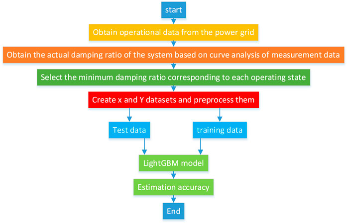
Figure 1. Model training flow chart.

This paper uses the system’s historical operating data to train the LightGBM model. The goal is to enable the model to accurately fit the relationship between the system’s operating state and its stability, thereby realizing real-time analysis of power system stability and quickly identifying whether the system has small-signal stability issues. The system is adjusted to a stable operating state through a correction model.

4.1 Input and output

Currently, the Wide Area Measurement System (WAMS) has been widely applied in power systems (Tang et al., 2020) and has become a crucial monitoring and control platform for power systems (Ju et al., 2019). WAMS is a dynamic monitoring and control system for power systems based on synchrophasor technology. Its core component is the Phasor Measurement Unit (PMU), which can use GPS signals to perform high-precision synchronous measurements of voltage and current in power systems, and provide information on frequency, phase, and amplitude. Composed of synchrophasor measurement devices, phasor data concentrators, control centers, and high-speed data communication networks, WAMS enables real-time monitoring and analysis of power grid status by deploying a large number of sensors and communication equipment in power systems. In this study, data measured by WAMS from the power system is used as input. Through curve analysis of the actual measured data, the actual damping ratio is obtained. The minimum damping ratio of each operating state is selected as the output.

${\xi }_{\min }$ should satisfy the following the inequality is Equation 13:

${\xi }_{\min }\ge {\xi }_{\text{limit}}(13)$

When the damping ratio is greater than ${\xi }_{\text{limit}}$, the system’s operating state is stable, and ${\xi }_{\text{limit}}$ is 0.03.

Take the power and minimum damping ratio measured from WAMS as input x and output y, respectively formulated as the input vector in Equation 14.

$x_k=\left[PL QL PG QG P_{ij} Q_{ij}\right],k=1,2,.....,n(14)$

The output is the minimum damping ratio, as shown in Equation 15:

$y_k=\left[{\xi }_{\text{mini}}\right],k=1,2,...,n(15)$

PL and QL are the active and reactive power of the load. PG and QG are the active and reactive power of the generator. ${\mathrm{P}}_{\text{ij}}$ and ${\mathrm{Q}}_{\text{ij}}$ refer to the line power from node i to node j. It refers to the minimum damping ratio for each operating state. N refers to the total number of samples. In addition to the power of the generator and load, the input part of this article also considers the line power to adapt to changes in the topology of the power grid. Establishing the relationship between input variable X and output variable Y through the LightGBM model, which are defined as the matrices in Equations 16, 17.

$X={\left[x_1{x}_2......x_n\right]}^T(16)$

$\mathrm{Y}={\left[y_1{y}_2......y_n\right]}^T(17)$

X is the set established by (13), and Y is the set established by (14).

4.2 Data processing and model evaluation methods

The input data is normalized using the Z-score method (Equation 18):

$x^{\prime }=\frac{x-\mu }{\sigma }(18)$

Among them: $x$ is the input value; $x^{\prime }$ is the value processed by normalization method; μ and σ are the mean and standard deviation of x.

After normalization of the input data, the problem of “large numbers overwhelming small numbers” caused by excessive absolute differences between data can be effectively prevented. For model evaluation, the Root Mean Square Error (RMSE) and Mean Absolute Percentage Error (MAPE) are adopted. RMSE reflects the deviation degree and distribution of errors, while MAPE represents the average value of relative errors. Their calculation methods are as follows, calculated using Equations 19, 20.

$\text{MAPE}=\frac{100\%}{n}{\displaystyle \sum _{k=1}^n}\left|\frac{y_k-\widehat{y_k}}{y_k}\right|(19)$

$\text{RMSE}=\sqrt{\frac{1}{n}{\sum }_{k=1}^n{\left(y_k-\widehat{y_k}\right)}^2}(20)$

Among them, n refers to the number of datasets, $y_k$ is the true value of the kth sample, and $\widehat{y_k}$ is the predicted value of the kth sample.

5 A small signal stability correction model based on LightGBM algorithm system

The damping ratio adjustment process is shown in Figure 2.

Figure 2

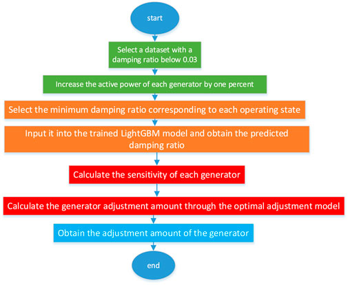
Figure 2. Generator power adjustment flow chart.

Select the damping ratio that is in an unstable operating state and correct it to a stable operating state with a damping ratio greater than 0.03 using the method mentioned above.

5.1 Calculation of damping ratio sensitivity

The calculation of damping ratio sensitivity can be determined by the output power $\Delta p_m$ of the generator during normal operation and the corresponding damping ratio $\Delta {\xi }_m$ to determine the sensitivity $\Delta \xi +\Delta {\xi }_m$ of the generator relative to the damping ratio, as well as the output power change $\Delta p+\Delta p_m$ corresponding to the change in damping ratio ($\Delta p_m$ is a slight disturbance, ranging from 0.01 to 0.1 pu), as shown in Equation 21.

$c_m=\frac{\Delta {\xi }_m}{\Delta p_m}(21)$

The total change in damping ratio is the sum of contributions from all generators (Equation 22):

$\Delta \xi =C_1\Delta P_1+C_2\Delta P_2+C_3\Delta P_3+.......+C_n\Delta P_n(22)$

n is the total number of generators in the system; $\Delta p_m$ is the active power adjustment corresponding to generator m; $\Delta \xi$ is the corresponding change in damping ratio of the system after adjusting the power generation of each unit (Wang et al., 2021).

5.2 Correction optimization model

In order to minimize the change in active power of each generator while achieving a damping ratio above ${\xi }_{\text{limit}}$, this section introduces an optimization model as follows this goal is formalized by the optimization model in Equation 23:

$\min {\displaystyle \sum _{i=1}^n}\Delta P_i^2(23)$

Subject to the following constraints (Equation 24):

$s.t.\left\{\begin{array}{l}{P}_i^{\min }\le P_{i_0}+\Delta P_i\le P_i^{\max }\\ {\xi }_0+\Delta \xi \ge {\xi }_{\text{limit}}\\ \sum _{i=1}^n{C}_i\Delta P_i=\Delta \xi \end{array}\right.(24)$

$\Delta P_i$ refers to the active power adjustment of generator $\mathrm{i}$, $P_{i_0}$ is the initial active power of generator $\mathrm{i}$, $P_i^{\min }$ and $P_i^{\max }$ are the lower and upper limits of the active power adjustment of generator $\mathrm{i}$, respectively.

6 Case study analysis

In this section, a 3-machine 9-bus system and a 10-machine 39-bus system are used for simulation verification. MATLAB is applied to simulate the actual operating states of the power systems. For each operating state, the active power and reactive power of generators, loads, and transmission lines, as well as the corresponding minimum damping ratio, are recorded. The collected data is used to train the LightGBM model. The dataset is divided into a training set and a test set in a ratio of 9:1.

This article uses random sampling to divide the training set and the testing set, with a ratio of 9:1. To ensure the model’s generalization ability to extreme operating conditions, we introduced random fluctuations in load and generator power during the data generation process, covering various operating scenarios of the system under normal and abnormal conditions.

6.1 3-Machine 9-node system with wind turbines

It includes 3 generators, among which the No. 3 generator is replaced by 60 wind turbines, and these wind turbines adopt a seventh-order model. Generators G1 and G2 use a sixth-order model with their excitation systems considered. The loads employ a constant impedance model, and changes in control parameters are not taken into account. To simulate both normal and abnormal operating states that may occur in actual power system operations, the active power (P) and reactive power (Q) of the generators are randomly fluctuated by 20%, and the system load is fluctuated by approximately 20%–30%. MATLAB is used to calculate the eigenvalues for each operating state, and 10,000 sets of data are generated through random oscillations. Randomly select 1,000 data points from 10,000 as the test set, and model and train the remaining 9,000 data points. The 3-machine 9-bus system is shown in Figure 3.

Figure 3

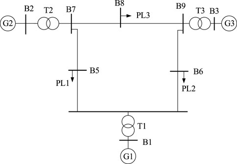
Figure 3. 3-machine 9-node system.

Bayesian optimization was performed on the parameters of LightGBM, and the final parameters are shown in Table 1.

Table 1

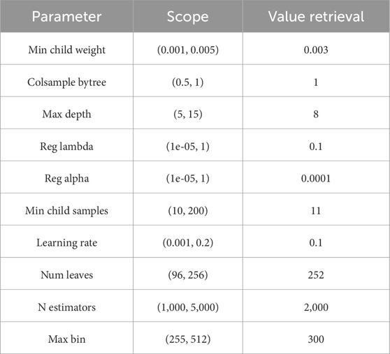
Table 1. Parameters of LightGBM model.

This article uses Bayesian optimization method to optimize the hyperparameters of LightGBM, and the selected parameters (as shown in Table 1) are determined based on their performance on the validation set. For example, num leaves controls model complexity, learning rate affects convergence speed, and max depth prevents overfitting. The combination of these parameters significantly improves training efficiency while ensuring prediction accuracy.

In practical power grids, the measurement error of data measurement units should be less than 1%. Therefore, the SNR is generally controlled above 30 dB (Nantian et al., 2021; Guanzheng et al., 2022). To verify the prediction ability of the proposed model under different noise conditions, Gaussian white noise of varying levels is added to the training data. MATLAB is used to generate Gaussian white noise with SNRs of 40 dB, 30 dB, and 26 dB, so as to evaluate the prediction accuracy of the three algorithms under interference. The prediction error graphs of three denoising algorithms are shown in Figure 4.

Figure 4

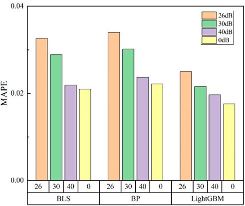
Figure 4. Prediction error of three algorithms adding noiset.

As shown in Figure 4, in the absence of noise, the MAPEs corresponding to the Generalized Learning System (BLS), Neural Network (BP), and LightGBM algorithms are 2.09%, 2.21%, and 1.75%, respectively. When there is a small fluctuation in the noise, there is a significant change in the relationship between the average error and the size of the noise. As shown in Table 2, under three different levels of noise, the average absolute error of the LightGBM algorithm is smaller than the prediction average error of BLS and BP.

Table 2

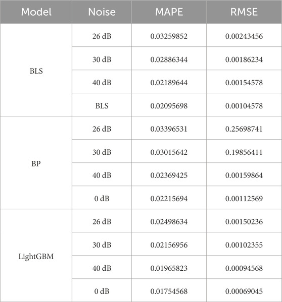
Table 2. Predictions of the three algorithms under different noises.

Figure 5 shows the prediction performance of the LightGBM model.

Figure 5

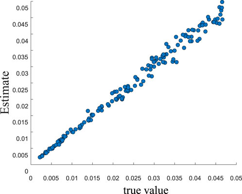
Figure 5. LightGBM model prediction results chart.

Figure 5 shows the comparison between the predicted and actual values of the minimum damping ratio of the system using the LightGBM model. The high agreement between the predicted curve and the true value indicates that the model has good fitting ability and generalization performance.

Table 3 shows the MAPE and training time of three algorithms. According to the data in the table, LightGBM outperforms BP and BLS in both training accuracy and speed.

Table 3

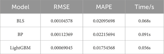
Table 3. Training results chart for the 3-machine 9-bus system.

ACC represents the percentage of adjustment error. The calculation formula is as shown in Equation 25:

$ACC=\frac{\left|{\xi }_{true}-{\xi }_{L\mathrm{i}ghtGBN}\right|}{{\xi }_{true}}(25)$

${\xi }_{true}$ refers to the actual damping ratio calculated after adjusting the active power of each generator, while ${\xi }_{L\mathrm{i}ghtGBM}$ is the damping ratio obtained by incorporating the adjustment into the LightGBM model.

The damping ratio sensitivity of generators is calculated based on the data-driven model. The perturbation amount of generators is set to 10%, and the ACC is within an acceptable range. The results of the damping ratio sensitivity of each generator estimated based on the LightGBM model are shown in Table 4.

Table 4

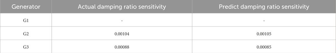
Table 4. Damping ratio sensitivity.

One set of data is randomly selected from the sample set with a damping ratio less than 0.03. The damping ratio adjustment is performed based on the calculated damping ratio sensitivity. Among them, Generator G1 serves as the system’s balancing unit and does not require adjustment. The minimum damping ratios after adjustment via the LightGBM prediction model and the optimization model are shown in Table 5.

Table 5

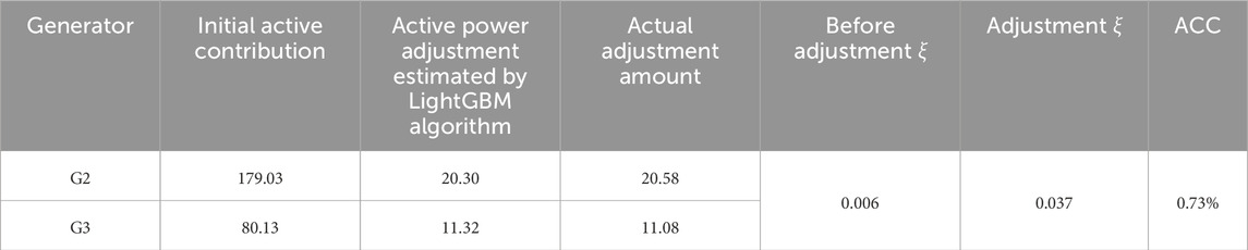
Table 5. Data table of the generator active power adjustment process and results.

6.2 10-Machine 39-node system with wind turbines

The 10-machine 39-bus system is shown in Figure 5. It comprises 10 generators, among which the No. 4 generator connected to Bus 33 is replaced by a wind farm aggregated from 320 wind turbines.

The other generators adopt a sixth-order model, with their excitation systems taken into account. The loads use a constant impedance model, and changes in control parameters are not considered. The wind turbines employ a seventh-order model. 10-machines with 39-nodes as shown in Figure 6.

Figure 6

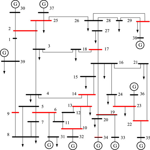
Figure 6. Ten-machine 39-bus system.

As shown in Table 6, the RMSE, MAPE, and training time of the three algorithms were compared in a 10 machine 39 node model.

Table 6

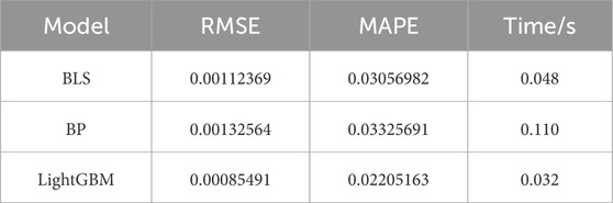
Table 6. Training results chart for the 10-machine 39-bus system.

Figure 7 shows the prediction performance of the LightGBM model.

Figure 7

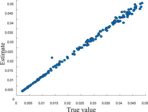
Figure 7. LightGBM model prediction results chart.

The predicted curve in Figure 7 is highly consistent with the true values, indicating that the model has good fitting ability and generalization performance in 10 machines and 39 nodes.

Gaussian white noise with signal-to-noise ratios (SNR) of 40 dB, 30 dB, and 26 dB is added to simulate the errors encountered when obtaining the minimum damping ratio in power systems. The Mean Absolute Percentage Error (MAPE) and Root Mean Square Error (RMSE) are used as indicators to evaluate the prediction accuracy of the models. The prediction accuracy of the three algorithms under different noise levels is assessed, and the prediction results are shown in Table 7.

Table 7

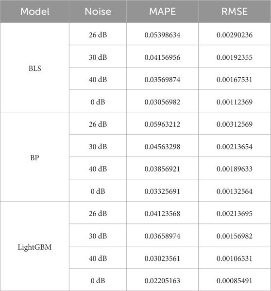
Table 7. Predictions of the three algorithms under different noises.

In the absence of noise interference, the Mean Absolute Percentage Errors (MAPE) of the BLS, BP, and LightGBM algorithms are 3.05%, 3.32%, and 2.21%, respectively. Their Root Mean Square Errors (RMSE) are 9.85 × 10⁻⁴, 11.23 × 10⁻⁴, 13.25 × 10⁻⁴, and 8.54 × 10⁻⁴ (note: there may be a typo in the original RMSE count, as it lists 4 values for 3 algorithms).

After adding Gaussian white noise with signal-to-noise ratios (SNR) of 40 dB, 30 dB, and 26 dB, the MAPE and RMSE of the four models (consistent with the RMSE count) all increase. Among them, the LightGBM model shows the most stable overall variation, as illustrated in Figure 8.

Figure 8

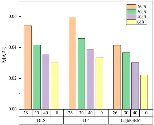
Figure 8. Prediction error of three algorithms adding noiset.

Table 8 shows the true damping ratio sensitivity of each generator and the predicted damping ratio sensitivity using LightGBM algorithm.

Table 8

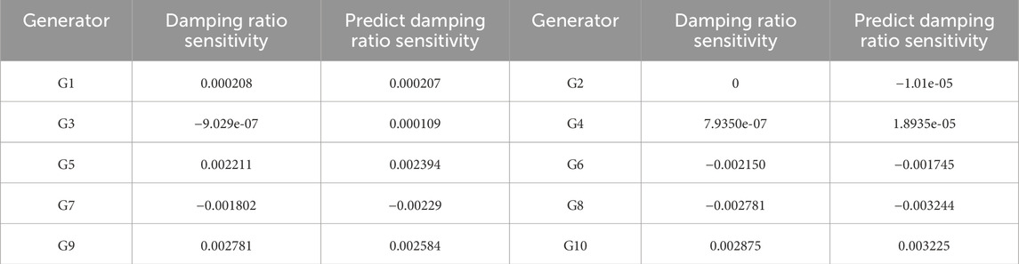
Table 8. Damping ratio sensitivity.

As shown in Table 9, the minimum damping ratio adjusted by the LightGBM prediction model and optimization model is 1.0554% for ACC.

Table 9

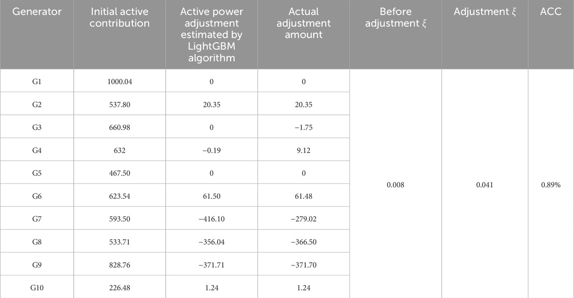
Table 9. Data table of the generator active power adjustment process and results.

7 Conclusion and future work

This paper evaluates the small-signal stability of power systems with wind power integration based on the LightGBM model. It also constructs an adjustment model by combining optimization algorithms to correct the power system from weakly damped operating states to stable ones. Tests are conducted on the 3-machine 9-bus system and the 10-machine 39-bus system. The simulation results show that the proposed method has high accuracy and fast adjustment response, while also verifying its feasibility in power system stability assessment and adjustment.

LightGBM features efficient computing performance and low memory usage. It supports automatic feature selection, missing value handling, parallel computing, and distributed training—these advantages enable it to exhibit significant strengths in processing large-scale data and significantly reduce preliminary data preprocessing work. Future research will focus on the following directions: combining LightGBM with physical models to construct more interpretable hybrid learning frameworks; Expand small disturbance stability analysis to multiple scenarios and time scales.

Data availability statement

The original contributions presented in the study are included in the article/supplementary material, further inquiries can be directed to the corresponding author.

Author contributions

YF: Writing – original draft. WG: Writing – review and editing. XY: Investigation, Writing – review and editing. MQ: Software, Writing – review and editing. AS: Data curation, Writing – review and editing. CJ: Methodology, Writing – review and editing.

Funding

The authors declare that no financial support was received for the research and/or publication of this article.

Acknowledgements

The authors would like to express their sincere gratitude to all the individuals and organizations that have supported this research.

Conflict of interest

Authors YF, WG, XY, MQ, AS, and CJ were employed by Guizhou Power Grid Co., Ltd. Power Dispatch Control Center.

Generative AI statement

The authors declare that no Generative AI was used in the creation of this manuscript.

Any alternative text (alt text) provided alongside figures in this article has been generated by Frontiers with the support of artificial intelligence and reasonable efforts have been made to ensure accuracy, including review by the authors wherever possible. If you identify any issues, please contact us.

Publisher’s note

All claims expressed in this article are solely those of the authors and do not necessarily represent those of their affiliated organizations, or those of the publisher, the editors and the reviewers. Any product that may be evaluated in this article, or claim that may be made by its manufacturer, is not guaranteed or endorsed by the publisher.

References

Bin, F., Yijie, H., and Gang, H. (2023). A review of novel dispatching and scheduling optimization methods for power systems based on deep reinforcement learning. Automation Electr. Power Syst. 47 (17), 187–199.

Google Scholar

Gibbard, M. J., Pourbeik, P., and Vowles, D. J. (2015). Small-signal stability, control and dynamic performance of power systems.

Google Scholar

Guanzheng, L., Bin, L., and Wang, S. (2022). Dynamic frequency prediction of power system after disturbance based on feature selection and random forest. Grid Technol., 1–12. doi:10.13335/j.1000-3673.pst.2021.0027

CrossRef Full Text | Google Scholar

Huang, M. Z., Hu, Y. H., and Weng, Y. F. (2021). A transient stability assess ment method for power systems incorporating jmim and ngboost. Autom. Electr. Power Syst. 45 (08), 155–165.

Google Scholar

Jia, H., and Yixin, Y. (2001). Chaos phenomena and related research in power systems. Chin. J. Electr. Eng. (07), 27–31.

Google Scholar

Jiang, H., Bai, Y., and Wang, S. (2021). Analysis method on the impact of wind power integration on small signal stability of power systems. Proc. CSEE 33 (09), 9–16. doi:10.19635/j.cnki.csu-epsa.000706

CrossRef Full Text | Google Scholar

Ju, Y., Sun, G., Chen, Q., Zhang, M., Zhu, H., and Rehman, M. U. (2019). A model combining convolutional neural network and LightGBM algorithm for ultra-short-term wind power forecasting. IEEE Access 7, 28309–28318. doi:10.1109/access.2019.2901920

CrossRef Full Text | Google Scholar

Ke, G., Meng, Q., Finley, T., and Chen, W. (2017). Lightgbm: a highly efficient gradient boosting decision tree. Proceeding Adv. Inf. Process. Syst., 3146–3154.

Google Scholar

Meng, J., Ming, W. M., and Zhang, L. (2005). Electromagnetic interference spectrum estimation for power converters based on modeling of igbt switching transient processes estimation of electromagnetic interference spectrum. CSEE J. Power Energy Syst. 37 (12), 14482–14498.

Google Scholar

Nantian, H., Wenguang, Z., and Guowei, C. (2021). Efficient identification of LightGBM power quality disturbances constrained by IoT data transmission rate. Chin. J. Electr. Eng. 41 (15), 5189–5201.

Google Scholar

Qu, Z., Li, H., Wang, Y., Zhang, J., Abu-Siada, A., and Yao, Y. (2020). Detection of electricity theft behavior based on improved synthetic minority oversampling technique and random forest classifier. Energies 13 (8), 2039. doi:10.3390/en13082039

CrossRef Full Text | Google Scholar

Saner, C. B., Yaslan Genc, Y. I., and Genc, I. (2021). An ensemble model for wide area measurement-based transient stability assessment in power systems. Electr. Eng. 103, 2855–2869. doi:10.1007/s00202-021-01281-x

CrossRef Full Text | Google Scholar

Tang, C., Luktarhan, N., and Zhao, Y. (2020). An efficient intrusion detection method based on LightGBM and autoencoder. Symmetry 12 (9), 1458. doi:10.3390/sym12091458

CrossRef Full Text | Google Scholar

Wang, Y., Chen, J., Chen, X., Zeng, X., Kong, Y., Sun, S., et al. (2021). Short-term load forecasting for industrial customers based on TCN-LightGBM. IEEE Trans. Power Syst. 36 (3), 1984–1997. doi:10.1109/tpwrs.2020.3028133

CrossRef Full Text | Google Scholar

Yanfeng, M. A., Zheng, L., and Huo, Y. (2020). Analysis on damping torque of virtual synchronous generators connected to power systems. Electr. Power Autom. Equip. 40 (04), 166–171. doi:10.16081/j.epae.202003027

CrossRef Full Text | Google Scholar

Yang, Y., Yu, L., and Yuan, H. (2017). Time domain calculation and waveform analysis of small signal stability in power systems. Adv. Technol. Electr. Eng. Energy 36 (01), 44–51. doi:10.13334/j.0258-8013.pcsee.2001.07.007

CrossRef Full Text | Google Scholar

Yin, B., Chen, Q., Li, B., and Zuo, L. (2021). A new method for identification and classification of power quality disturbance based on modified kaiser window fast s-transform and lightgbm. Proceed CSEE 41 (24), 8372–8384.

Google Scholar

Zeng, D., and Jun, Y. (2020). Frequency small-signal stability analysis of multi-machine parallel systems with virtual synchronous generators. Proc. CSEE 40 (07), 2048–2061. doi:10.13334/j.0258-8013.pcsee.191217

CrossRef Full Text | Google Scholar

Zhang, R., Wu, J., and Baoqin, L. (2020). Adaptive prediction of transient stability in power systems based on transfer learning. Grid Technol. 44 (06), 2196–2205. doi:10.13335/j.1000-3673.pst.2019.2376

CrossRef Full Text | Google Scholar

Zhou, T., and Yang, J. (2016). Power system transient stability assess ment method based on modified lightgbm. Power Syst. Technol. 43 (6), 1931–1940.

Google Scholar