 George J. Adams
 Richard B. Cook
 John R. Hutchinson
 Peter Zioupos
- 1Cranfield Forensic Institute, Cranfield University, Defence Academy of the United Kingdom, Shrivenham, United Kingdom
- 2National Centre for Advanced Tribology at Southampton (nCATS), Faculty of Engineering and the Environment, University of Southampton, Southampton, United Kingdom
- 3Structure and Motion Laboratory, Department of Comparative Biomedical Sciences, Royal Veterinary College, University of London, Hatfield, United Kingdom
An understanding of bone apparent and material densities and how they vary within bone at the organ level is of great interest in the understanding of degenerative bone conditions and for biomedical engineering applications. The densities of bone tissue have been shown to appreciably influence the mechanical competency of bone tissue. In order to assess the density of bone in the body, it is important to ensure that the parameters being measured in vivo are truly representative of the real values that have been measured in vitro. To assess the densities of bone across the entire spectrum of available porosities, 112 samples from an elephant femur were assessed using the Archimedes method (water displacement) and by micro-computed tomography (μ-CT). Comparisons were drawn between the two methods to determine if the densities calculated by μ-CT were representative of physically measured densities. The results showed that the apparent densities measured over the entire spectrum were very similar but varied in the intermediate regions of bone tissue, probably due to an increased presence of osteoid, increased remodeling, or experimental error as these type of bone is known for the presence of regions of closed cell geometry in the cancellous architecture. It could be argued that the measurements taken by μ-CT are more reliable of bone density values for the mineralized regions of bone as the threshold is defined with respect to the absorption of X-rays by the mineral. In contrast, the Archimedes method thresholds everything with a density value above that of the surrounding medium, 1 (g cm−3) for water, and hence it is more sensitive to the presence of osteoid, soft collagenous matrix, and epithelial cell layers. Further research is required to optimize the parameters of scanning methods for the structural properties of different bone tissue porosities, which hopefully in turn will be able to provide a basis for the development of predictive remodeling models.
Introduction
Bone, the material, exists at the organ level as whole bones. Whilst bone may seem relatively inert compared with other structures in the bone it is in fact an adaptive material which responds to its environment. The fundamental results of Wolff’s Law hold true but his explanation and understanding of the underlying mechanisms were misunderstood (Currey, 2002). The nature of the biological and micro-mechanical mechanisms that drive bone remodeling is still not fully understood. At its material level, bone is a multiphase composite material formed of both organic and inorganic constituents. It has a hierarchical structure that ranges from the sub-nano level of the collagen-mineral composite through to the macro-structure of cortical and cancellous bone.
The density and structure of bone are important characteristics that determine its mechanical behavior in everyday life. An understanding of these underpinning properties is crucial in the investigation of bone as a structural material. Density can be defined in a number of ways ranging from the micro- to the macro- or organ level. The two generally accepted versions of density are the “apparent” and “material” ones. Apparent density (Dapp) is the mass of the mineralized tissue over the total volume occupied by the tissue with the inclusion of its voids. The most common representation of Dapp used in respect to bone is bone mineral density (BMDa) which, when measured by dual energy X-ray diffraction (DEXA), is an area assessment of this characteristic. Material density (Dmat) is defined as the same mass as for apparent density divided by the volume the solid mineralized tissue occupies with the exclusion of any voids that may exist within the structure. The most popular use of this is often referred to as tissue mineral density. These definitions highlight that the difference between these properties is the consideration of mass with respect to the micro-structure of the tissue, such as: voids, osteocyte lacunae, osteonal canals, and analogous non-mineralized architectural features:
where BV is the bone volume and TV is the total volume. The assessment of densities within bone tissue is considered to be important as it will impact upon the resultant mechanical properties and remodeling characteristics of bone (Martin, 1984; Fyhrie et al., 1993; Zioupos et al., 2008). The derivation of Dapp is not contested because it is simply the wet bone mass of a sample over the Cartesian geometric volume occupied by the same bone sample. Different methods for material density, however, have caused some debate (Schileo et al., 2008; Zioupos et al., 2008). The most conventional technique employed for this assessment relies on the Archimedes principle (usually via water displacement). Application of this method relies critically on ensuring that pores must be fully flushed and refilled (Zou et al., 1997). This flushing and refilling are particularly difficult in cases where there are cells of closed geometry within the trabecular architecture (Rho et al., 1995). Comparisons of DEXA and the Archimedes technique have previously reported substantial differences (Keenan et al., 1997) whilst fractional quantitative and cone beam computed tomography has been shown to be in closer agreement with Archimedes (Lee et al., 2004; Ahlowalia et al., 2013). When investigating Dapp and Dmat, consideration must be given to the volume of bone or BV/TV (dimensionless ratio of actual bone volume to the total volume of the sample). This can be calculated with the Archimedes principle using Eq. 3. Calculating BV/TV with the Archimedes method depends therefore in ensuring that the displaced suspending medium (water, a solution of known density, or a gas) infiltrates all the pores and thus derives the true BV for the sample. BV/TV has also been calculated/measured by using a series of histological slices (Martin, 1984). This technique can also carry an inherent error due to the limitation of physical slice thickness which requires interpolation between each slice; in the addition to sample destruction.
The Dapp is often considered to be one of the primary characteristics of bone that influence its mechanical properties at the macro-mechanical level and has been shown to influence not only the compressive but also the fracture toughness properties of bone (Rice et al., 1988; Cook and Zioupos, 2009). Dmat determines material behavior primarily at the trabecular level. However, due to the fact that Dapp is the product of Dmat × BV/TV, it determines properties at the structural level too. A previous study has shown, in elephant bone samples, that the relationship between Dapp and Dmat are interdependent and that Dmat is at its highest (~2.3g cm−3) value at the extremes of porosity, as BV/TV tends toward 1 and 0, and exhibits minimum values at intermediate levels of BV/TV of 0.4–0.7 (Zioupos et al., 2008).
This relationship has, however, been brought into question when it was suggested that the actual shape of it may be due to limitations of the Archimedes method in the assessment of bone tissue material density (Schileo et al., 2009) because, as commented earlier, the method depends on ensuring that the displaced suspending medium infiltrates all the pores and thus derives the true BV of a sample. To overcome this limitation, μ-CT can be used as it gives information on the internal structure, it is non-destructive and it can penetrate throughout the material so that marrow-filled spaces and more enclosed cells are accessible and thus these will not affect the results. Some previous work has looked at the density relationship applied at cortical and cancellous regions using μ-CT (Schileo et al., 2008), but it has not considered bone densities throughout the entire range with particular attention to the intermediate range of densities. The present study, therefore, aims to test the hypothesis that, when applied to the same bone tissue samples, Archimedes and μ-CT can produce effectively the same results and also to explore the implications of μ-CT derived data in mechanobiology studies.
Materials and Methods
Specimens
In this study, 112 samples were taken from the right femur of an adult Asian elephant (3,432 kg, 24 years old). The specimen was collected shortly after the animal’s euthanasia (for reasons unrelated to this study) at Whipsnade Zoo (Bedfordshire, UK) and frozen (−20°C) until sample testing. Whilst use of elephant tissue is not ideal for human applications, is does have certain advantages as it is mammalian with the shape and properties at the bone matrix level (confirmed by nano-indentation tests in our laboratories; unpublished data) similar to those of a human femur, the only major difference, therefore, being one of size. This large size enabled extraction of extensive volumes of cortical and cancellous bone which allowed structural effects similar to human tissue to be observed on a scale in tens of millimeters; additionally, it enabled production of all cortical and cancellous samples from the same sections throughout the same bone (no intra- or inter-individual variability), and obtained from a sample from an animal known to have previously been healthy. The samples had been characterized in a previous study (Zioupos et al., 2008), where full details of sample extraction can be found.
μ-CT Imaging
All samples were imaged using a cone beam μ-CT scanner, XTEK CT H 225 (Nikon Metrology, Nottingham, UK). The samples were imaged in ABS plastic sample holders (~1-mm thick) at 50 kV, 65 µA with a 500 ms exposure time. The resultant voxel size was ~16 μm, making them suitable to accurately determine the samples’ morphology (Yan et al., 2011). Each sample was imaged twice. First they were imaged fully submerged in deionized water. The samples were then imaged again in air. All image data were manually reconstructed using CT Pro 3D. With CT Pro the beam hardening and noise reduction filters were applied to provide an optimal image; this image setting was then standardized across the data set to ensure that the data collected were comparable.
Image Analysis
Image analysis was carried out using VG Studio Max 2.2. Regions of interest were taken from the center of each sample ~9 mm3 to exclude any external surfaces from the calculations. A surface determination was performed using the gray level of an internal void as the background and the largest void-less section of bone as the sample gray value, as per the manufacturers’ recommendations. After the surface determination, an automatic morphometric report was exported which contained: BV/TV, specific surface, mean trabecular thickness, mean trabecular number, and mean trabecular spacing.
From the histogram, the mean, mode, minimum, and maximum gray levels were recorded to be used in calculation of the material density. A QRM-MicroCT-HA calibration phantom was scanned and reconstructed under the same conditions in order to determine Dmat. Determination of material density is more favorable than deriving Hounsfield units (HU) in this context as HU provides a relative density based on the attenuation coefficients of the material that cannot be measured by traditional densitometry. However, density as mass per unit volume can easily be compared with physical densitometry techniques.
Density Calibration
A histogram of the QRM HA calibration phantom alongside the 3D image of the scan is shown in Figure 2. Both the histogram and image were obtained using VG Studio Max software. Within the software, each density was isolated and the average gray scale was determined and plotted against the density provided by the supplier. This provided a calibration curve [a least squares regression equation: density (g cm−3) = 1.099 + (0.0015 + gray value)] from which the density of the elephant samples could be determined. The average gray value of each sample was measured, and using the calibration curve, Dmat was determined for each sample.
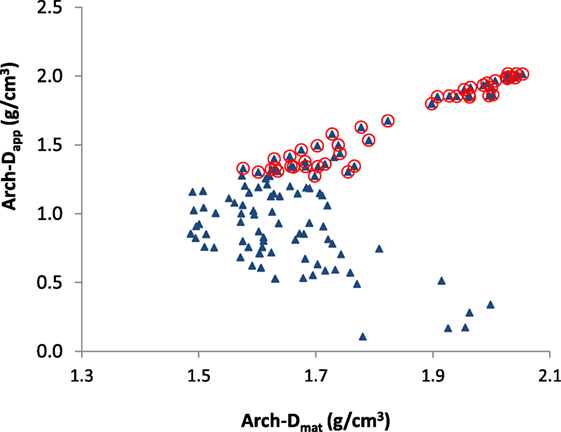
Figure 1. Apparent (Dapp) vs. material density (Dmat) for all samples (triangles) produced from the same femur in both cortical and cancellous regions, adapted from Zioupos et al. (2008). The samples having Dapp > 1.3, which on visual inspection would be identified as cortical bone regions, are encircled and the same notation is used in the following figures to allow visual comparisons to be made between figures. Material density (Dmat) showed lower values for intermediate BV/TV values in the range of 0.4–0.7. “Arch” denotes the measurements were obtained in a study using the Archimedes method.
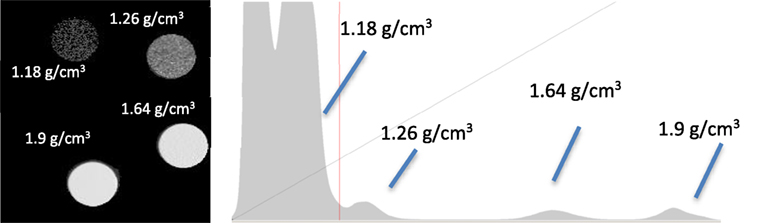
Figure 2. QRM calibration phantom images and histogram; the average density, gray, and mineral % are given in Table 1.
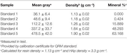
Table 1. Properties of QRM calibration phantom.
The Dapp was determined from the product of the BV/TV and Dmat by rearranging Eq. 3. In the present study, to distinguish between measurements taken from CT and measurements taken using the Archimedes technique, the prefixes CT- and Arch- are used, respectively.
A comparison of two possible methods for determination of density is shown in Figure 3. Density can either be taken from the average gray value in the sample or from the center of the peak on the histogram, which represented the modal gray value for the sample. Each method has advantages and disadvantages. Measuring the mean gives the average gray value; however, it inevitably includes voxels that are only partially filled with bone caused by the partial voxel effect, which can skew the mean to be less than the true mean. Taking the center of the peak avoids this issue related to partial volumes but only takes the most common density in the scan and has the potential to ignore a non-uniform distribution of densities around the mode.
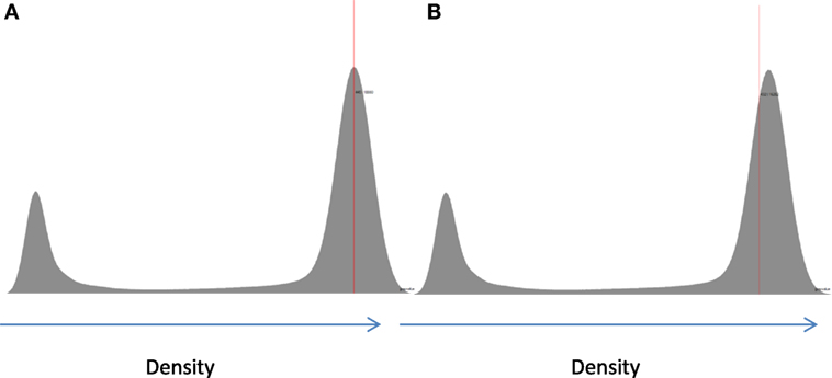
Figure 3. Example of two possible ways to determining the material density from the histogram for a cortical bone sample: (A) taking a measurement of the peak value (mode) and (B) taking the mean value above the determined threshold.
Inevitably, and as shown in Figure 3, the mode value taken will always be higher than the mean value due to the non-zero regions between the background, in this case water, and the bone peak. As such, taking the measurement from the mode value is unaffected by the background, which would suggest that it is the best method to use. However, this cannot be applied uniformly across the whole range of porosities. For extremely porous cancellous bone, there is very little bone from which to quantify the gray level (density) and then taking a measurement from the center of the bone peak is extremely difficult. In these few cases, using the mean value is the most suitable option so that a reliable density variable can be obtained across the entire cohort (Figure 4). The examples in Figures 3 and 4 serve to illustrate the considerable difficulties in obtaining reliable density values from gray levels in the CT across the whole BV/TV range in bone. Similar to Archimedes, the CT method is not, therefore, without its own limitations. Indeed, another argument could be that the integrated pixel values should be used to quantify density, which would take into account any partial voxels (i.e., only partly occupied by bone) that otherwise cannot fully be taken into account with the prior two methods. We focus here on those other two methods but a future study using the integrated pixel values would be interesting.
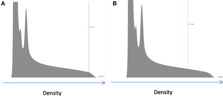
Figure 4. Example of two possible ways to determining the material density from the histogram for an extremely porous cancellous bone sample: (A) taking a measurement of the peak value; the location of the peak value is approximated due to the lack of a resolved peak in the low-BV/TV samples; (B) taking the mean value above the determined threshold. There is a high score for low-density voxels on the left-hand side of the histogram which correspond to water, fat, marrow, remnants of blood clots, and other such contaminants in the samples.
Results
The full results of the way densities compare with each other, when measured by the mode or the mean value of gray levels (after appropriate and specific thresholding of the voxels), are in Figure 5. The material density calculated by the mean underestimates the value produced by the mode, as expected, but the two are very well linearly correlated with each other (Figure 5). There are also very few outliers where the two values deviate considerably for some difficult samples, but these do not spoil the overall pattern nor do they cast a strong shadow of doubt on the very principle of measuring bone densities across the complete range of porosities. The symbols encircled in red are, as is our practice, those for the cortical bone samples. Once again, as in the original paper using the Archimedes method (Zioupos et al., 2008), there is an underlying regressive behavior of the sample density, which goes down and up as bone goes from dense cortical to porous cancellous between these two extremes and which is can be appreciated by the arrows added manually on the graph.
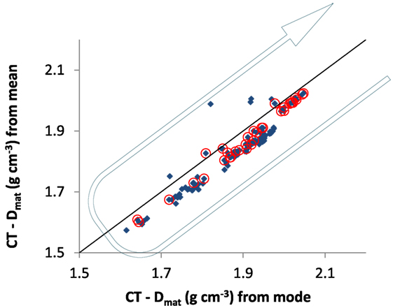
Figure 5. Comparison of estimating material density by the “mean” and “mode” gray levels of the bone samples. The line shown represents a slope of one and goes through zero, for illustrative purposes. Some outliers exist where there is little bone in the scan so the “mode value” does not lie near the center of the “mean value.” The arrow points to the underlying regressive behavior of the sample material density, which goes down and up as bone goes from dense cortical to porous cancellous between the two extremes of BV/TV.
A comparison of the CT-Dapp measured from the mean and Arch-Dapp by the laboratory method of Zioupos et al. (2008) is shown in Figure 6. The plot has a slight inflection in the intermediate bone density values. If we consider that Arch-Dapp is a more reliable method because it is simply the wet weight over the bone sample volume, then it appears that CT-Dapp underestimates apparent bone density in these intermediate value regions as it is based on the absorption of X-rays from mineralized tissue alone. Data for Arch-Dapp are produced empirically using a microbalance to measure wet weight of the bone and Vernier calipers to measure volume. Arch-Dapp is in essence the method for apparent density that is used in every biomechanical lab globally to produce Modulus of Elasticity = f(Apparent Density) relationships. The data show that there is “bone” matter which is not captured or quantified by the CT-Dapp variable, and this matter is most likely be the lower density non-mineralized portions of the bone samples in remodeled areas, practically regions of osteoid tissue in its various stages toward full skeletal maturity.
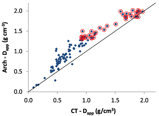
Figure 6. Comparison of Dapp from Zioupos et al. (2008) vs. Dapp measured by CT in the present study (on the same samples). Otherwise, the description in Figure 5’s caption applies.
The comparison of BV/TV measurements shown in Figure 7 demonstrates that the Arch-BV/TV measured in the laboratory is higher in the intermediate regions, most likely due the fact that the Archimedes measurements consider all tissue including the un-mineralized layers on the surface of the tissue. It is most apparent in the intermediate region as it is a surface effect, and in the intermediate regions there is the greatest amount of specific surface available (Martin, 1984; Berli et al., 2017) for the volume of bone.
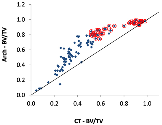
Figure 7. Comparison of the BV/TV ratio measured by μ-CT with previous reported BV/TV values measured by Zioupos et al. (2008) (“Arch-BV/TV”) for the same samples. Otherwise, the description in Figure 5’s caption applies.
The results of Figures 6 and 7 are in agreement with each other as to what disparities exist between the methods. These low-density regions on the surfaces of bone are due to the remodeling of bone where the “younger” bone regions are less mineralized. Microscope images displaying localized structural properties of bone are shown in Figure 8 and are widespread in the literature. Figure 9 depicts graphically the “mosaic” of tissue compartments that bone is at any point in time. These compartments are regions of varying mineral contents at various temporal points in the development of the mineralization process that leads from osteoid formation to mature, fully mineralized bone.
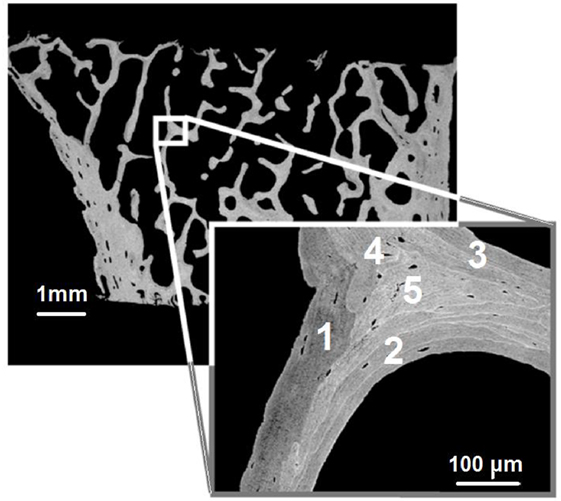
Figure 8. Microscope images showing the mosaic of different layers of bone tissue with progressively denser mineralization levels (adapted and modified from original in Ruffoni et al., 2007). Based on gray level alone, one would have numbered the various tissue compartments as 1 being the more recent, toward 5 being the older one.
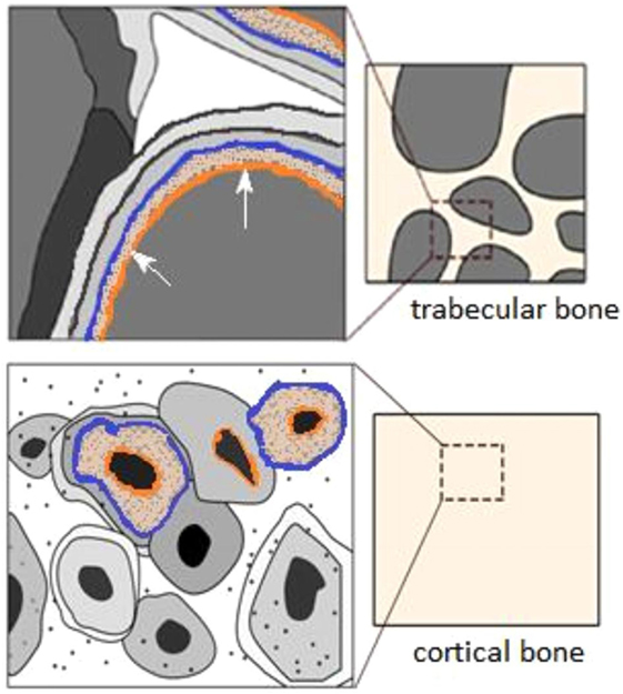
Figure 9. Graphic displaying the remodeling regions of bone tissue in cancellous and cortical bone adapted from Berli et al. (2017) with proposed possible thresholds which have been added to image for the Archimedes (1.0 g cm−3) (orange) and μ-CT thresholds (1.3 g cm−3) (blue), for the soft collagenous boundary and osteoid tissue, respectively.
Figure 10 shows the “boomerang”-like pattern previously shown by Zioupos et al. (2008) is now apparent in both Archimedes-based and μ-CT-produced data. The μ-CT-produced curves do, however, have shallower inflection points: the lowest Arch-Dmat is ~1.48 g cm−3 as opposed to 1.60 g cm−3 for CT-Dapp. The shallower inflection point is due to higher values for measured Dmat in the intermediate bone porosities when μ-CT is used. In views of the previous arguments and graphs, these higher values for Dmat most likely exist for two possible reasons: (i) the density measured by the Archimedes method is skewed by the presence of approximately closed voids in the cancellous bone matrix, which would overestimate the volume to bone if they are not fully flushed for the marrow they contain (in the calculation of Dmat = weight/volume a higher volume will lead to a reduced Dmat whereas in μ-CT these voids do not impact on the data) and/or (ii) the surface of cancellous bone in Archimedes measurements is thresholded at a density of 1 g cm−3 (because it displaces water in the Archimedes tests), thus including low-density epithelial layers and newly forming osteoid, but this same soft organic material does not possess a density high enough to register in the μ-CT measured density. The disparity between the measurements most likely exists due to a combination of these factors. The differences between the measurements are also apparent in Figures 6 and 7, which shows a clear inflection in the intermediate range of bone densities. The apparent density measured via Archimedes is undisputed and seems to carry less error than any other physical method—a statement that is open to interpretation (measurement of actual weight and of physical dimensions with calipers). However, we conclude that it is the μ-CT method, not so much the Archimedes method, that needs particularly cautious attention for potentially misleading technical errors. In both ways for both methods, the “boomerang”-like pattern is strongly evident.
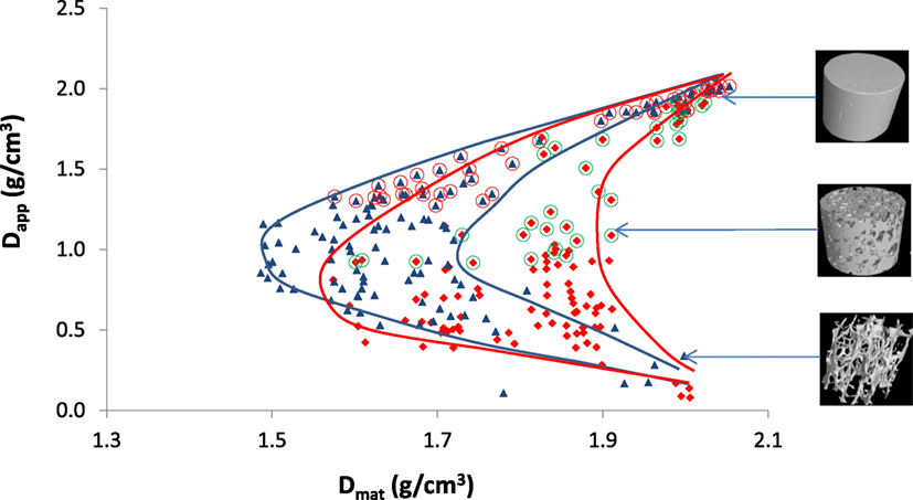
Figure 10. Apparent vs. material density for all samples throughout the whole range from cortical to cancellous bone. Blue triangles are produced by the Archimedes method (Zioupos et al., 2008), the red diamonds are from μ-CT, and the lines showing the envelopes were manually added around the two data sets. 3D reconstructed images of samples are shown on the right at their respective densities.
Discussion
Here, we have furthered the investigation into the basic relationships that exist between apparent and material density values within bone in both its cortical and cancellous forms, and throughout its whole porosity range. Bone densities directly impact upon the mechanical competency of the tissue (Rho et al., 1995; Zioupos et al., 2008). Understanding the behavior of bone density across the full range of porosity values is vitally important for the comprehensive understanding of remodeling behavior and remodeling rates at specific sites within the human body (Martin, 1984; Fyhrie et al., 1993). Such density data will contribute to future development of patient-specific finite element modeling, which depends on accurate assessment of the material properties of the tissue and its structure (Chevalier et al., 2007; Schileo et al., 2008). Conflicting reports have been made on the nature of the density variations across the full porosity range (Schileo et al., 2008, 2009; Zioupos et al., 2008), which, however, used different methods to assess the same property and on different samples. Assessing these bone properties has typically been carried out by means of histological measurements (sectioning) and traditional densitometry techniques such as the Archimedes technique (Martin, 1984; Rho et al., 1995; Zou et al., 1997; Zioupos et al., 2008). These methods are destructive and can be criticized for their limitations in reproducibility, which is most likely due to their inability to guarantee full penetration of the sample using various solvents, which has led some studies to use a gas pycnometer (helium displacement method; Zou et al., 1997).
μ-CT imaging has its own limitations which interfere with density measurements, too. In μ-CT imaging, it is important to ensure that image resolution is suitable for the size and structures being assessed. In this study, the imaging resolution was sufficient for determination of cancellous micro-architecture but not for further assessment of the vascular nano-micro-architecture, which is at a range <1 μm (Yan et al., 2011). This is an important consideration when looking at the specific surface of bone, because when looking at cellular sites for bone remodeling the cortical bone may be more porous than the results here would suggest and consequently the reported remodeling rates would be also affected. Additionally, the densities presented in this work were calculated in grams per cubic centimeter to provide comparison between the two methods. In contrast, for clinical relevance HU would be of greater value, which have been shown to be suitable when using cone beam micro-computed tomography (Mah et al., 2010). Moreover, in μ-CT imaging consideration must also be given to the methods of density determination; be it by the “mean” or “mode” values of the gray value distribution (or other approaches as noted above in Section “Materials and Methods”); as in highly porous samples determination of both can be problematic, and as shown by Figure 4 there is a deviation in the produced values in such cases of very porous bone material.
This study’s findings have confirmed the trend of data from experiments on the same collection of samples used by Zioupos et al. (2008). These samples when using the Archimedes density determination method showed a highly non-linear relationship between Dmat and Dapp for bone across all porosities and showed an inflection in the data in the intermediate regions between cortical and cancellous bone (Figure 1). The results from both methods (Figure 10) agree in the shape of the curve but differ in the magnitude of the non-linearity. The difference is understandable in that the two methods (one mechanical; one physical) use different physical principles and measure bone density differently. The limitation of a μ-CT scan is that it assesses density indirectly through the absorption of X-rays by the hard matter of bone (Schileo et al., 2008; Mah et al., 2010) and thus it certainly ignores the soft organic matrix. The limitations of the Archimedes method is that it requires repeated measurements and very careful preparation for cancellous samples with more closed cell architecture where the suspending medium (usually water) does not penetrates fully the entire space. In spite of these differences, both data sets are in agreement of a “boomerang” like effect which is prominent (density variation between high and low values of at least 37%) and is certainly not a constant value for Dmat across the whole range as claimed by Schileo et al. (2008, 2009).
In bone histology, less dense regions of bone are typically considered to be younger bone which in turn suggests that the intermediate porosity regions, which here are shown to contain bone of lower material density, do so because they experience higher rates of remodeling. The work of Berli et al. (2017) has attributed this to a process which is a surface-moderated effect, whereby the greater the specific surface area available, the higher the remodeling rate and the lower the mineral density due to the increased formation and presence of osteoid. The results also confirm that μ-CT based measurements of density, which are pursued for the purpose of scanning bones for micro-FEA, ought to use relationships between gray level/density/modulus of elasticity that are produced by micro-mechanics (e.g., nano-indentation tests) at the same magnification level and not the commonly provided ones produced at a macro-mechanical level (Morgan et al., 2003). Micro-mechanical tests are needed for micro-mechanical level data for micro-FEA because the bone material density fluctuates with porosity and does not maintain a constant value as has been assumed in past studies. This is shown by Figure 11. Erroneous material data values can be assigned if elastic modulus vs. density relationships from the literature [E = f(D)], which have been produced at a macro-mechanical level, are assigned to bone at the voxel size level for micro-FEA. When the voxel size is smaller than the bone pore size, for instance, if the voxel is at a void the E value is zero, if it is where bone mass is, the modulus value should be a function of the bone mineralization level and of only this.
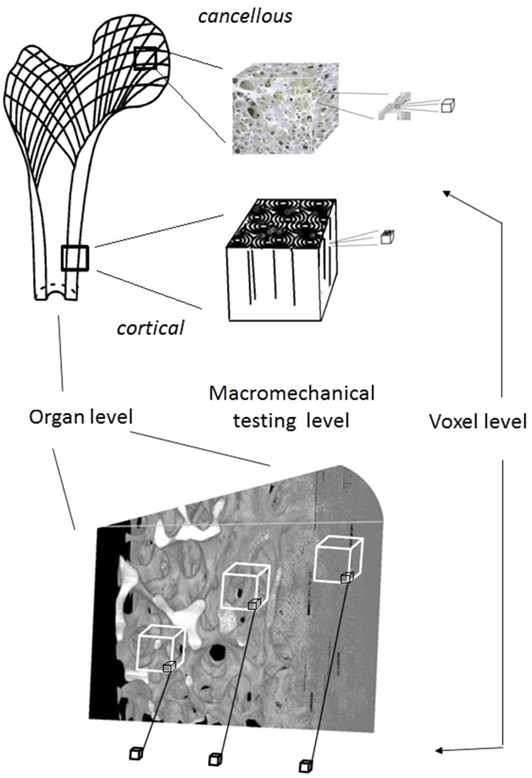
Figure 11. Material property assignment is performed on relationships produced by mechanical testing at the macro-mechanical level. However, at voxel scales the relationship is one of (E) = f(mineral level) instead and as the present study has demonstrated this level is dependent on the level of BV/TV too. Consequently, in micro-FEA studies the assignment of E = f[gray level = f(%mineral)] should be made via appropriately conducted studies for tests (by using nano-indentation, for instance, Wolfram et al., 2010) at this magnification level.
Conclusion
This study has shown that bone material density varies non-linearly with bone apparent density across the full spectrum of bone porosities. We have provided further evidence in favor of density-dependent material models for the future development of patient-specific finite element models. Additional care must be taken when setting thresholds and sampling the material density—it is recommended that further work be carried out into the impact of setting μ-CT sampling thresholds on the material data. More investigation is needed into the source of the disparity, where it exists, between data obtained from the Archimedes and μ-CT methods. Additionally, the micro-architectural properties of bone across all porosities should be investigated more carefully because this may allow more profound inferences into the development of remodeling models.
Ethics Statement
The study was approved by institutional Cranfield University Research & Ethics committee.
Author Contributions
GA, JH, RC, and PZ design the study. GA performed the study. GA, RC, and PZ analyzed the results. GA and PZ wrote the manuscript. GA, RC, JH, and PZ had equal contribution to the paper.
Conflict of Interest Statement
The authors have no commercial or any other financial relationship or any conflict of interest to declare in conjunction with the work presented in this paper.
Funding
The tests were carried out in the Biomechanics laboratories of the Cranfield Forensic Institute of Cranfield University in Shrivenham, UK. The authors are thankful to Professor Michael Fagan for supplying the QRM HA calibration standard, Dr. Michael Doube for helpful comments on an earlier draft of this paper, the EPSRC (GR/N33225; GR/N33102; GR/M59167), the BBSRC (BB/C516844/1), the Department of Comparative Biomedical Sciences (RVC) for financial support and ZSL Whipsnade Zoo for provision of the specimen.
References
Ahlowalia, M. S., Patel, S., Anwar, H. M., Cama, G., Austin, R. S., Wilson, R., et al. (2013). Accuracy of CBCT for volumetric measurement of simulated periapical lesions. Int. Endod. J. 46, 538–546. doi: 10.1111/iej.12023
Berli, M., Borau, C., Decco, O., Adams, G., Cook, R. B., García Aznar, J. M., et al. (2017). Localized tissue mineralization regulated by bone remodelling: a computational approach. PLoS ONE 12:e0173228. doi:10.1371/journal.pone.0173228
Chevalier, Y., Pahr, D., Allmer, H., Charlebois, M., and Zysset, P. (2007). Validation of a voxel-based FE method for prediction of the uniaxial apparent modulus of human trabecular bone using macroscopic mechanical tests and nanoindentation. J. Biomech. 40, 3333–3340. doi:10.1016/j.jbiomech.2007.05.004
Cook, R. B., and Zioupos, P. (2009). The fracture toughness of cancellous bone. J. Biomech. 42, 2054–2060. doi:10.1016/j.jbiomech.2009.06.001
Fyhrie, D. P., Fazzalari, N. L., Goulet, R., and Goldstein, S. A. (1993). Direct calculation of the surface-to-volume ratio for human cancellous bone. J. Biomech. 26, 955–967. doi:10.1016/0021-9290(93)90057-L
Keenan, M. J., Hegsted, M., Jones, K. L., Delany, J. P., Kime, J. C., Melancon, L. E., et al. (1997). Comparison of bone density measurement techniques: DXA and Archimedes’ principle. J. Bone Min. Res. 12, 1903–1907. doi:10.1359/jbmr.1997.12.11.1903
Lee, J., Shin, H. I., and Kim, S. Y. (2004). Fractional quantitative computed tomography for bone mineral density evaluation: accuracy, precision, and comparison to quantitative computed tomography. J. Comput. Assist. Tomogr. 28, 566–571. doi:10.1097/00004728-200407000-00022
Mah, P., Reeves, T. E., and McDavid, W. D. (2010). Deriving Hounsfield units using grey levels in cone beam computed tomography. Dentomaxillofac. Radiol. 39, 323–335. doi:10.1259/dmfr/19603304
Morgan, E. F., Bayraktar, H. H., Tony, M., and Keaveny, T. M. (2003). Trabecular bone modulus–density relationships depend on anatomic site. J Biomech. 36, 897–904. doi:10.1016/S0021-9290(03)00071-X
Rho, J. Y., Hobatho, M. C., and Ashman, R. B. (1995). Relations of mechanical properties to density and CT numbers in human bone. Med. Eng. Phys. 17, 347–355. doi:10.1016/1350-4533(95)97314-F
Rice, J. C., Cowin, S. C., and Bowman, J. A. (1988). On the dependence of the elasticity and strength of cancellous bone on apparent density. J. Biomech. 21, 155–168. doi:10.1016/0021-9290(88)90008-5
Ruffoni, D., Fratzl, P., Roschger, P., Klaushofer, K., and Weinkamer, R. (2007). The bone mineralization density distribution as a fingerprint of the mineralization process. Bone 40, 1308–1319. doi:10.1016/j.bone.2007.01.012
Schileo, E., Dall’ara, E., Taddei, F., Malandrino, A., Schotkamp, T., Baleani, M., et al. (2008). An accurate estimation of bone density improves the accuracy of subject-specific finite element models. J. Biomech. 41, 2483–2491. doi:10.1016/j.jbiomech.2008.05.017
Schileo, E., Taddei, F., and Baleani, M. (2009). Letter to the Editor referring to the article “Some basic relationship between density values in cancellous bone and cortical bone” published on Journal of Biomechanics (volume 41, Issue 9, Pages 1961–8). J. Biomech. 42, 793. doi:10.1016/j.jbiomech.2009.01.013
Wolfram, U., Wilke, H. J., and Zysset, P. K. (2010). Valid micro finite element models of vertebral trabecular bone can be obtained using tissue properties measured with nanoindentation under wet conditions. J. Biomech. 43, 1731–1737. doi:10.1016/j.jbiomech.2010.02.026
Yan, Y. B., Qi, W., Wang, J., Liu, L. F., Teo, E. C., Tianxia, Q., et al. (2011). Relationship between architectural parameters and sample volume of human cancellous bone in micro-CT scanning. Med. Eng. Phys. 33, 764–769. doi:10.1016/j.medengphy.2011.01.014
Zioupos, P., Cook, R. B., and Hutchinson, J. R. (2008). Some basic relationships between density values in cancellous and cortical bone. J. Biomech. 41, 1961–1968. doi:10.1016/j.jbiomech.2008.03.025
Keywords: bone, cancellous, cortical, density, porosity, BV/TV, micro-computed tomography
Citation: Adams GJ, Cook RB, Hutchinson JR and Zioupos P (2018) Bone Apparent and Material Densities Examined by Cone Beam Computed Tomography and the Archimedes Technique: Comparison of the Two Methods and Their Results. Front. Mech. Eng. 3:23. doi: 10.3389/fmech.2017.00023
Received: 03 October 2017; Accepted: 21 December 2017;
Published: 05 February 2018
Edited by:
Gianluca Tozzi, University of Portsmouth, United KingdomReviewed by:
Alexandre Terrier, École Polytechnique Fédérale de Lausanne, SwitzerlandKatherine A. Staines, Edinburgh Napier University, United Kingdom
Copyright: © 2018 Adams, Cook, Hutchinson and Zioupos. This is an open-access article distributed under the terms of the Creative Commons Attribution License (CC BY). The use, distribution or reproduction in other forums is permitted, provided the original author(s) and the copyright owner are credited and that the original publication in this journal is cited, in accordance with accepted academic practice. No use, distribution or reproduction is permitted which does not comply with these terms.
*Correspondence: Peter Zioupos, cC56aW91cG9zQGNyYW5maWVsZC5hYy51aw==