 N. Swaminathan
- Department of Engineering, Cambridge University, Cambridge, United Kingdom
MILD combustion is gaining interest in recent times because it is attractive for green combustion technology. However, its fundamental aspects are not well-understood. Recent progresses made on this topic using direct numerical simulation data are presented and discussed in a broader perspective. It is shown that a revised theory involving at least two chemical timescales is required to describe the inception of this combustion not only showing both autoignition and flame characteristics but also a strong interaction between these two phenomena. The reaction zones have complex morphological and topological features and the most probable shape is pancake-like structure implying micro-volume combustion under MILD conditions unlike the sheet-combustion in conventional cases. Relevance of the MILD (micro-volume) combustion to supersonic combustion is explored theoretically and qualitative support is shown and discussed using experimental and numerical Schlieren images.
1. Introduction
The world total primary energy supply (TPES) has increased from 6.2Btoe (Billion ton of oil equivalent) in 1973 to about 13.8Btoe in 2016 (International Energy Agency, 2019)1. This 220% increase over a period of 43 years will continue further and more than 90% of this supply comes from combustion of coal, oil, gas, or renewable biomasses. Figure 1 shows the future projections of potential combustion share of TPES under three different scenarios. The inset is the actual data from International Energy Agency (2019) showing a gradual drop of the combustion share and a small rise in 2012 is because of the increase in coal combustion in some of the countries around the world. If one naively projects this data by assuming that the progress in technology to replace combustion for meeting the energy demand is steady and organic following the current trends then the combustion share is likely to be more than 80% even by the year 2070 (the curve with open triangle). The slope of this curve is related to the progress and advancement of alternative energy technologies. If one keeps an optimistic view for the non-combustion technologies progressing at 50% faster pace compared to the current trend then the combustion share falls just below 80% by 2070. This share decreases to 77% by the year 2070 even if one assumes that the alternative technologies progress at 70% faster pace, which is a highly optimistic view. It seems that a radical paradigm shift is required for a significant reduction of the combustion share and whether this is practical or not is an open question. A pragmatic approach to mitigate combustion impact on the environment is to seek for alternative combustion concepts and technologies which can significantly reduce CO2 and other pollutants emission and can also be employed as retrofits into the existing systems. Fuel-lean and MILD (moderate, intense, or low dilution) combustion concepts emerge as potential solutions.
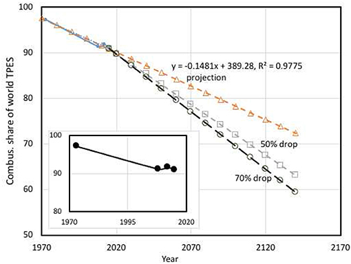
Figure 1. The contribution of combustion to world TPES and its future projection.
The interest here is on MILD combustion because of its ability to simultaneously reduce pollutants emission and increase overall thermal efficiency (Wünning and Wünning, 1997; Cavaliere and de Joannon, 2004). The efficiency gain comes from the energy recovered by recirculating hot gases and the emission reduction is because of reduced oxygen level in and temperature rise across combustion zones under MILD conditions. This mode of combustion is said to occur when the fuel-air mixture temperature, Tr, is higher than the reference auto-ignition temperature, Tign, for a given mixture and the temperature rise, ΔT = (Tb − Tr), is smaller than Tign (Cavaliere and de Joannon, 2004), where Tb is the burnt gas temperature. These two conditions are typically achieved by diluting the fuel-air mixture with exhaust gases and the dilution level is controlled carefully to keep the oxygen level typically below 5% by volume. If one uses (Tr − Tign) and ΔT − Tign as two axes as suggested by Cavaliere and de Joannon (2004) then the MILD combustion locates in the fourth quadrant and this is sketched in Figure 2 with pictures representing typical combustion types identified (Doan, 2018). The temperature raise, ΔT is larger than Tign for HiTAC and conventional (Feedback) combustion whereas it is smaller than Tign for the MILD and pilot-assisted combustion. The MILD combustion has Tr − Tign > 0 since the reactant temperature is larger than Tign. Typically, one expects the autoignition process to be dominant under this condition but direct numerical simulation (DNS) studies showed the presence of autoignition fronts with premixed and non-premixed flames and also their interactions (Minamoto, 2013; Doan, 2018). This challenges the use of conventional flame theories and models for MILD combustion.
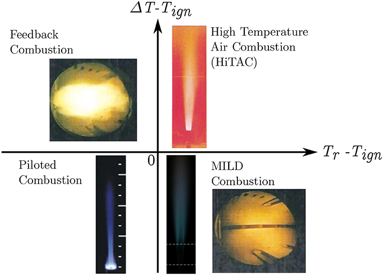
Figure 2. A diagram showing various combustion types: HiTAC (Fujimori et al., 1998), feedback or conventional (de Joannon et al., 2000), piloted (Dunn et al., 2010), and MILD (de Joannon et al., 2000; Medwell et al., 2007) combustion. This diagram is adapted from Doan (2018) under a Creative Commons license.
The heat release rate in this combustion is distributed spatially yielding a homogeneous temperature field with no visible flame (Katsuki and Hasegawa, 1998; de Joannon et al., 2000; Ozdemir and Peters, 2001; Minamoto and Swaminathan, 2014b; Sidey and Mastorakos, 2015; Sorrentino et al., 2016) and thus the MILD combustion is also called as “flameless” combustion. These features are atypical of conventional combustion having strong heat release in thin regions leading to inhomogeneous temperature or density field. DNS studies showed that some features of conventional combustion are also present under MILD conditions (Minamoto and Swaminathan, 2014b; Doan and Swaminathan, 2019b). Furthermore, the chemical kinetics plays a strong role in the inception of MILD combustion which can lead to some unconventional behaviors of reaction zones in response to scalar dissipation (or fluid dynamic strain) rate (Doan and Swaminathan, 2019c). Hence, the objective here is to survey the past DNS studies on MILD combustion and provide a broader perspective on MILD combustion physics by answering the following questions
1. What is the inception mechanism for MILD combustion?
2. What is the main combustion mode, autoignition or flames, under MILD conditions or is it a mixed mode combustion?
3. What are the typical morphological and topological features of reaction zones in MILD conditions?
4. What is the simplest way to model MILD combustion?
Since these questions are of fundamental nature, analysing DNS data is the best possible way to answer them. Also, it is worth to note that the modern combustion concepts such as Homogeneous Charge Compression Ignition (HCCI), Reactivity Controlled Compression Ignition (RCCI), and Gasoline Compression Ignition (GCI) for automotive engines may share some common features with MILD combustion. The next section reviews the DNS data briefly. The insights gained in many past studies are reviewed and discussed in section 3 to answer the above questions. The tentative modeling ideas arising from the physical insights are presented in section 4 and the relevance of MILD combustion to supersonic combustion, which is a topic of long-standing interest for high-speed air transport, is discussed in section 5. The conclusions are summarized in the final section.
2. DNS of MILD combustion
Direct numerical simulation of turbulent combustion under MILD conditions is not common and only two research groups have attempted this in the past using two different flow configurations. van Oijen (2013) and his co-workers (Göktolga et al., 2015) considered ignition in a temporally evolving turbulent mixing layer between counter-flowing fuel and hot oxidant streams to mimic the flow and reacting features of jet-in-hot-coflow burner of Adelaide (Dally et al., 2002) operating under MILD conditions. The results of these studies suggested that autoignition occurred at the most reactive mixture fraction, ZMR, with different ignition delays depending on temperature and scalar dissipation rate experienced locally by the most reactive mixture. Also, the molecular diffusion of heat and mass were shown to be important and thus 3D simulations are inevitable to understand MILD combustion physics.
The DNS studies at Cambridge considered a cubic domain with carefully constructed flow and mixture conditions mimicking MILD combustion with recirculated hot exhaust gases. These simulations were conducted in two stages for computational economy. The first stage considered the mixing of reactants/fuel-air mixture with hot exhaust gases while the second stage involved combustion as shown in Figure 3. Both premixed (Minamoto, 2013) and non-premixed (Doan, 2018) MILD combustion were studied. For non-premixed MILD combustion, typically oxidant stream is diluted using the hot exhaust gases as shown schematically in Figure 3 and this is called as hot-oxidant and diluted-oxidant by de Joannon et al. (2012). The DNS procedures are described in detail by Minamoto and Swaminathan (2014b) for premixed and by Doan et al. (2018) for non-premixed cases, and a brief summary is given below.
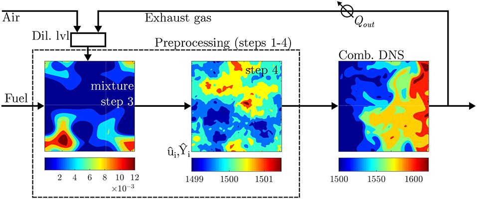
Figure 3. A schematic of DNS steps followed for non-premixed MILD combustion with internal recirculation of exhaust gases, adapted from Doan et al. (2018) under a Creative Commons license.
The initial and inflowing fields of mixture fraction, Z, reaction progress variable, c, scalar mass fractions, Yα, and velocity fields, ui, were generated in 5 preprocessing steps marked in Figure 3 without step 5. Bilger mixture fraction was used to define Z (Bilger et al., 1990) and the reaction progress variable was based on fuel mass fraction. A decaying homogeneous isotropic turbulence was simulated in step 1 to obtain the turbulence field inside the computational domain. Laminar MILD premixed flames for various Z values were computed and the scalar mass fractions were tabulated as a function of Z and c in step 2. Initial turbulent mixture fraction and reaction progress variable fields were constructed with prescribed means, 〈Z〉 and 〈c〉, and lengthscales, ℓZ and ℓc in step 3. Only the progress variable field was considered for the premixed cases. The step 4 mapped the species mass fractions Yα(c, Z) obtained in step 2 onto the initial mixture fraction and progress variable fields. The turbulence and scalar fields obtained respectively in steps 1 and 4 were allowed to interact in step 5 for about one large eddy turnover time, 40 μs, of the initial turbulence field. This step is not shown in Figure 3. This time is much shorter than the time, 140 μs, required for the normalized temperature cT = (T − Tr)/(Tb − Tr) to increase by about 10% in a perfectly stirred reactor having a mixture representative of volume-averaged DNS condition. The scalar fields obtained at the end of step 5 included unburnt, c = 0, burnt, c = 1 and also partially burnt, intermediate values of c, mixtures with equivalence ratio, ϕ, varying from 0 to 10 inside the computational domain for non-premixed cases and it was fixed to be 0.8 for the premixed cases. These preprocessed fields were then used as the initial and inflowing conditions for the MILD combustion DNS in the second stage shown in Figure 3. Elaborate details are discussed by Minamoto and Swaminathan (2014b) and Doan et al. (2018).
The combustion kinetics was described using MS-58 mechanism involving 19 species and 58 reactions (Doan et al., 2018), which was a modified version of Smooke and Giovangigli mechanism (Smooke and Giovangigli, 1991) with OH* chemistry from Kathrotia et al. (2012). The elementary reactions with OH* precursors were taken from KEE-58 mechanism (Bilger et al., 1990). This combined mechanism is validated in detail by Doan et al. (2018). The premixed MILD combustion DNS used Smooke and Giovangigli mechanism without OH*.
The thermochemical conditions of the MILD mixture used for the DNS are listed in Table 1. Since methane is used as fuel for these mixtures the reference ignition temperature is about Tign = 900 K. The mixtures NP-M1 and NP-M3 are for non-premixed cases whereas the other two mixtures are for premixed cases. The air is diluted for the non-premixed MILD combustion (see Figure 3) whereas the fuel-air mixture is diluted for the premixed cases. The diluted mixture temperature is kept to be Tr = 1, 500 K, which is comparable to that used in the experiments of Suzukawa et al. (1997). These conditions suggest that the combustion is strictly in the MILD regime of Figure 2. The conditions of three non-premixed and three premixed turbulent MILD cases are listed in Table 2. The non-premixed cases are simulated by Doan et al. (2018) and premixed cases are from the study of Minamoto and Swaminathan (2014b). The cases NP1 and NP2 used the mixture NP-M1, which has the same O2 level as for P-M3 and these two turbulent cases differed by the lengthscale ratio, ℓZ/ℓc. The case of ℓZ/ℓc < 1 was not considered because the mixing length scale for mixture fraction field is generally larger than the chemical length scales such as the flame thickness or ignition kernel size at Tr as large as 1,500 K. The mixture NP-M3 with 2% of O2 was used for the turbulent case NP3. The premixed cases P1 and P2 had the same dilution level as in the mixture P-M1 but different turbulence conditions – P1 had which gave the Damköhler and Karlovitz numbers to be 1.72 and 4.78, respectively, whereas the case P2 had (3.8, 12.3) yielding 3.25 and 2.11 for the Damköhler, , and Karlovitz, , numbers. The case P3 had the same turbulence as for P1 at the inlet but used more diluted mixture P-M3 and hence the combustion characteristics are Da = 0.69 and Ka = 11.9. The burning velocity and Zeldovich flame thickness of the freely propagating laminar premixed flame used in the step 2 of the preprocessing step for the premixed MILD cases are SL and δf, respectively. The RMS of velocity fluctuations in the initial turbulence field with an integral length scale Λ0 is u′. Table 2 lists the characteristics of the initial scalar fields relevant for the discussion in this paper. Further detail can be found in the studies of Minamoto and Swaminathan (2014b) and Doan et al. (2018).
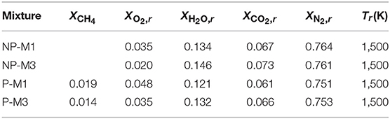
Table 1. Thermochemical condition of the oxidizer for MILD mixture.
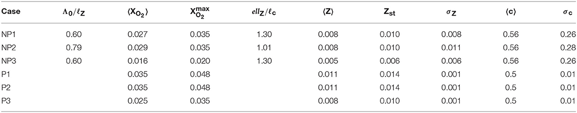
Table 2. DNS initial conditions.
The cubic domain of size Lx × Ly × Lz = 10 × 10 × 10 mm3 with inflow and non-reflecting outflow boundary conditions in the x-direction and periodic conditions in the transverse, y and z, directions was used. The domain was discretized using 512 × 512×512 uniformly distributed grid points which ensured that all chemical and turbulence lengthscales were resolved for the three non-premixed and, P1 and P2 premixed cases. For the case P3, 384 grid points were used in all three directions. The DNS code SENGA2 solving fully compressible conservation equations for mass, momentum, internal energy, and species mass fractions, Yi, was used. These simulations were made on HECToR and ARCHER, the UK national high performance computing facility. Other detail such as numerical scheme, computational time, etc., can be found in the studies of Minamoto (2013) and Doan (2018).
3. Insights
Figure 4 shows the normalized heat release rate, , iso-surface having a value of 2. For the premixed case, the normalizing quantities are taken from a MILD flame element (laminar MILD flame) having an equivalence ratio of 0.8 whereas for the non-premixed case the local equivalence ratio is used to get the normalizing thermo-chemical quantities. This result is shown at about 1.5τf, where τf is the flow through time defined as the ratio of computational domain length Lx to the mean velocity, Uin, at the inlet boundary. The figure on the left is for the premixed MILD case P3 and on the right is for the non-premixed case NP1 and these two cases have almost the same dilution level and overall equivalence ratio. Thus, the overall temperature rise, which is about 200 K, is the same for these two cases and hence the temperature variation across the domain is shown only for the non-premixed case NP1. Typical thickness of local zones with strong heat release can be seen to be thin in some parts of domain and thick zones can also be seen in other parts visible in Figure 4. It is also observed that heat release (chemical reactions) occur in extremely convoluted zones distributed over a very large portion of the computational domain in both cases. This increases the possibility for interactions of reaction zones and clearly differentiates MILD combustion from conventional combustion having a clear flame front with localized heat release. Furthermore, reactions occur near the entrance of the computational domain, shown by the presence of the iso-surfaces there (see Figure 4), which is due to the elevated temperature of incoming stream with radicals initiating reactions.
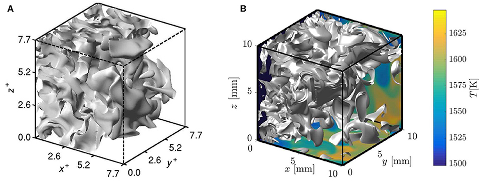
Figure 4. Iso-surface of normalized heat release rate of 2 from (A) P3 and (B) NP1 MILD combustion cases. The temperature field is shown in the bottom and side surfaces in (B). The axes are normalized using the laminar flame thermal thickness for the premixed case P3. These figures are adapted from Minamoto (2013) for P3 and Doan (2018) for NP1 cases under a Creative Commons license.
Although there are some minor differences in the spatial distribution of the heat release, the overall pattern is more or less the same in these two cases. Hence, there is no difference whether the MILD combustion occurs in premixed or non-premixed mode as long as the turbulence and mixture thermo-chemical conditions are kept to be similar. This is not so for conventional combustion in premixed and non-premixed modes as it is well-known that the combustion is concentrated around the stoichiometric mixture fraction in non-premixed conventional combustion. The striking similarity is interesting and advantageous for developing MILD combustion models. However, there are complexities such as frequent and abundant interaction of reaction zones which are not easy to deal with in the classical turbulent combustion modeling such as flamelets, flame surface density approaches. Further insights on these points are discussed in section 4.
3.1. MILD Combustion Inception
The conventional non-premixed combustion aspects such as ignition (inception) and extinction are studied typically using S-curves which are constructed by solving steady flamelet equation in the mixture fraction space (Pitsch and Fedotov, 2001). This equation is
with NZ, st as the mixture fraction scalar dissipation rate (SDR) at stoichiometry and its reference value is . The normalized temperature is θst = (Tst − Tst, r)/(Tst, p − Tst, r) = (Tst − Tst, r)/ΔTst. The normalized reaction is written for a one-step reaction and it involves a Damköhler number, , normalized activation temperature, β = Ta, eff/Tst, p, and heat release factor α. The exact form of this expression is not required here but can be found in earlier studies (Pitsch and Fedotov, 2001; Doan and Swaminathan, 2019c). A root which satisfies the above equation is obtained for given values of , β and various other parameters. The variation of θst with obtained thus for , α = 0.679 βref = 8.03 and 5 different values of β is shown in Figure 5A. The ignition and extinction points are also marked in this figure. There is no stable combustion between these two critical points and they move toward each other as β decreases leading to a monotonic increase of θst as NZ, st decreases, which can be seen for β = 2 and 4 in the figure. The inception region is highlighted using an ellipse in Figure 5A, showing a drop in the normalized temperature as the SDR (mixing rate) increases. This behavior is contrary to what is observed for the inception of MILD combustion in the DNS results shown in Figure 5B for the three non-premixed cases. The symbols represent the variation of doubly conditioned SDR obtained as 〈NZ|θst, Zst〉 = ∫NZ P(NZ|θst, Zst) dNZ with θst, where P is the probability density function (PDF) of SDR conditioned appropriately. One can also consider 〈NZ|θ〉 vs θ which is also shown in the figure. These results are constructed using samples collected over the entire sampling period of 1.5τf. It is clear that the normalized temperature increases with mixing rate or SDR in the inception stage. This is because of the presence of radicals such as OH promoting chemical reactions in the incoming mixture which is absent for one-step reaction used for the S-curve analysis.
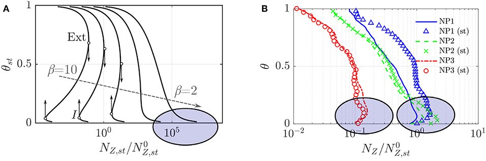
Figure 5. Variation of normalized temperature at stoichiometry location with the corresponding mixture fraction dissipation rate in (A) conventional non-premixed and (B) turbulent MILD non-premixed combustion. The variation of 〈NZ|θ〉 with θ constructed using the entire DNS sample is also shown in (B) using lines. These figures are adapted from Doan and Swaminathan (2019c) under a Creative Commons license.
The importance of OH becomes more apparent if one plots with θ. The symbol is the local value of the incoming OH mass fraction when there is no combustion, alternatively this is the local value due to convective-diffusive transport of the incoming OH mass fraction. This was obtained by performing a DNS with the same initial and inflowing fields as the MILD combustion cases but with no chemical reaction (Doan and Swaminathan, 2019a,c). Thus, ΔYOH < 0 means that OH coming from the inlet is consumed and ΔYOH > 0 implies that OH is produced locally. Since the interest is in the inception stage of MILD combustion, the variation of ΔYOH with corresponding θ is shown in Figure 6 for the samples collected from the first 5% of the computational domain in regions with large heat release rate, which are marked using . The normalized temperature increase is seen only in the regions with negative ΔYOH implying the key role played by the incoming OH in the inception of MILD combustion. This leads to the increase of θ with NZ seen in Figure 5, which is different from the S-curve behavior. Hence, an alternative theory giving due importance for the role of chemical kinetics in the formation and consumption of radicals such as OH is required for MILD combustion. Such a theory is yet to be developed and it seems that at least two chemical time scales may be required to investigate the physics of MILD combustion inception.
Figure 6. (A) Variation of ΔYOH with θ for sample collected in the initial 5% of the computation domain and with at an arbitrarily chosen time for the case NP1. The line denotes 〈θ|ΔYOH〉, adapted from Doan and Swaminathan (2019c) with permission. (B) PDF of ΔYOH conditioned on for the case NP1 at an arbitrarily chosen time, adapted from Doan and Swaminathan (2019a) under a Creative Commons license.
The PDF of ΔYOH conditioned on the heat release rate is depicted in Figure 6B for the case NP1 at an arbitrarily chosen time. The nine curves shown are for ranging from 0.1 to 0.9, where is the maximum heat release rate observed in the data. The PDF shows a bimodal behavior for low heat release rate; the peak at negative ΔYOH is because of the OH in the incoming stream and thus they signify the unreacted mixtures whereas the peak at positive ΔYOH is for the product mixtures. The bimodal PDF shifts gradually into a monomodal PDF for locations with large heat release rate. The OH-PLIF (planar laser-induced fluorescence) commonly used for the combustion diagnostics will pick the signals, coming from mixtures with low heat release, corresponding to the right peak and is likely to miss the signals from regions with large heat release rate since YOH is almost the same as the background value, . Thus, one needs extra care for studying MILD combustion using PLIF techniques (Doan and Swaminathan, 2019a).
3.2. Flame or Ignition?
From the fundamental perspective, the flame is established where there is convective-diffusive-reactive balance for the local scalar flux. When this balance is compensated by the temporal derivative (unsteady) term then the flame propagates. If there is ignition then typically the mixture is homogeneous locally and thus the convective and diffusive fluxes are small compared to the contributions from reactive and unsteady terms of the species balance equation. All of these can be seen quite clearly if one writes the balance equation for species i using standard notations:
where . For a closer understanding of local flux-balance, one may write and hence implies a steady flame-like structure locally while suggests an ignition-like structure and a positive value of signifies propagating flame. The ambiguity may arise for if there exists purely convective-diffusive type balance, which can be eliminated by conditioning on the normalized heat release rate, . This analysis has been done in the past and some of those results are shown in Figures 7, 8 to aid the discussion here. Minamoto et al. (2014) showed that ignition fronts and flames are present and also there are regions with entangled flame and ignition. This is depicted in Figure 7, where represents value normalized using ρr, SL and δth for the mixture used for the turbulent premixed case P3. It is apparent that the MILD combustion involves conventional features like flames and autoignition in some regions and also these two features can coexist in some other regions of the flow. This is a unique aspect of MILD combustion and which attribute is favored locally depends on the scalar gradient driving the various fluxes. Minamoto and Swaminathan (2014b) showed that the scalar gradient in the direction normal to the reaction zone is as strong as the tangential gradients in MILD combustion which is contrary to the conventional combustion showing stronger normal gradient compared to the tangential components [see Figure 11 of Minamoto and Swaminathan (2014b) and Figure 5.5 of Minamoto (2013)] for the premixed MILD combustion cases, P1 to P3 in Table 2. Similar behaviors were observed for the non-premixed cases NP1 to NP3. The time evolution of these attributes and their structures are studied by Doan et al. (2018) and Doan and Swaminathan (2019b). An example of this complex evolution is shown in Figure 8 depicting the Lagrangian tracks of few fluid parcels colored using values. It is quite normal to see an ignition fronts evolving into steady or propagating flames in conventional combustion which is also seen in Figure 8. The intriguing and also quite unusual behavior observed in the figure is the evolution of a flame-like structure into ignition-like behavior as one moves along a particular track, which is indicated by the changing from its positive to negative value. This is because of mixing and burning of unburnt mixtures of varied equivalence ratio in non-premixed cases and a close interaction between scalar mixing and chemical reactions. Overall, the MILD combustion is observed to display both autoignition and flame characteristics and a strong interaction between them.

Figure 7. Typical contours of (color map) are shown along with flame dominated (, white contours) and reaction dominated (, black contours) regions from the case P3. The results are shown for the mid x-y plane at an arbitrarily chosen time. Typical reaction and flame dominated regions are marked respectively using a black box and a white box with solid lines, which are enlarged at bottom right and top right respectively. Several regions showing entangled reaction and flame characteristics are marked using black boxes with dashed lines and one of such region is enlarged on the side, adapted from Minamoto (2013) under a Creative Commons license.
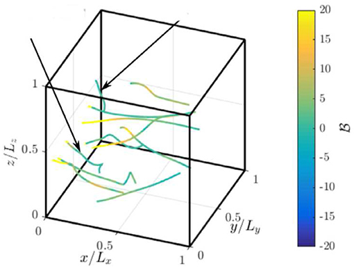
Figure 8. Evolution of along Lagrangian tracks of chosen fluid parcels and the tracks are drawn for a duration from 1 to 1.5τf. This results is shown for the case NP3 in Table 2, adapted from Doan (2018) under a Creative Commons license.
Takeno index, which is related to the gradients of fuel and oxidizer, can be used to delineate non-premixed and premixed reaction zones present in non-premixed MILD combustion. This analysis showed that the contributions to the overall heat release from premixed and non-premixed modes are comparable and the contribution of rich premixed mode decreased for the highly diluted case, NP3, compared to the case NP1 (Doan et al., 2018). The contribution of lean premixed mode did not change much between these two cases but the non-premixed mode contribution nearly doubled for NP3 compared to the NP1 case. Doan et al. (2018) also reported that the ignition front-like structures contributed about 25%, which is not small, to the overall heat release. The physical picture emerging from these insights is that the non-premixed MILD combustion involves rich and lean premixed zones, non-premixed zones and ignition front-like structures. A similar picture was also observed for premixed MILD combustion but without non-premixed zones (Minamoto et al., 2014).
3.3. Typical Morphological and Topological Features of Reaction Zones
Reaction zones can be identified using a threshold for but Minamoto (2013) suggested that the conditional average of the heat release rate weighted by the scalar dissipation rate of reaction progress variable, Nc, and surface area, , and conditioned on , i.e., , is more suited to identify heat releasing zones in MILD combustion. The surface area, ΔS, is identified using and the value of ξ+ corresponding to served as a suitable threshold to identify heat releasing zone iso-surfaces in various cases investigated. A typical reaction zone identified using this method is shown in Figure 9A for the premixed case P1 and this is not a simply connected surface which is commonly seen in conventional turbulent premixed combustion. Also, this iso-surface is observed to enclose a volume and there are holes, indicated by the arrows, and this volume is extending over a good portion of the computational domain. It is not easy to characterize this reaction zone using the common shapes such as sheet, ribbon, tube, and blob. However, one can unambiguously define three length scales for any 3D objects using Minkowski functionals and there are 4 functionals for a 3D object (Minkowski, 1903), which are given by Sahni et al. (1998)
where is the volume enclosed by the iso-surface S identified as above having a surface area of . The two principal curvatures at a given point on S are κ1 and κ2 (κ1 ≥ κ2). These four functionals are Galilean invariant morphological properties of the object, the reaction zone identified as above. The fourth functional is the Euler characteristics of the object and thus it is related to the genus of the object (Leung et al., 2012; Minamoto et al., 2014). Now, the three length scales ordered as T < W < L are defined using these four functionals as (Sahni et al., 1998)
These scales are representative and do not give the exact dimensions in the three directions except for a sphere of radius r for which T = W = L = r. Two shape finders, known as planarity P and filamentarity F can be defined using these three length scales and are given by Sahni et al. (1998)
Figure 9B shows the typical values of P and F for the reaction zones extracted from the cases P1 to P3 at an arbitrarily chosen time. For the sake of comparison, the values for the reaction zones of a conventional premixed flame are also shown in the figure. The premixed flame reaction zones have large P and relatively lower F values implying that these zones have sheet-like morphology, which is well-known. A wide range of P and F values is observed for the MILD reaction zones with the most probable values of P≃0.4 to 0.5 and F≃0.15 to 0.25. These most probable values suggest that the MILD reaction zones are like pancakes although there are reaction zones which are blob-like (very small values of P and F). Also, the topology, which refers to the connection, of MILD reaction zones are complex, see Figure 7. The non-premixed cases NP1 to NP3 showed similar variations for P and F. Hence, the MILD reaction zones are not simply-connected surfaces as in the conventional combustion and they have complex morphological and topological features, which are quite challenging for modeling.
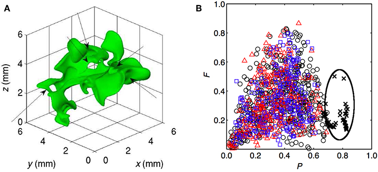
Figure 9. (A) Morphology of a typical heat releasing zone in the MILD combustion case, P1. (B) Values of shape finder, P and F, in the cases P1 ◦, P2  , P3
, P3  , and conventional premixed combustion × , adapted from Minamoto (2013) under a Creative Commons license.
4. Modeling
Minamoto and Swaminathan (2014a) showed that these complex features, specifically interaction of reaction zones, pose challenges for flamelet-based modeling approaches. However, if one treats the local reaction zones as a collection of perfectly or well-stirred reactors (PSR or WSR) then the statistical variations of major and minor species mass fractions and mean reaction rates can be captured quite well. This was demonstrated by Minamoto and Swaminathan (2014a) for RANS approach and by Minamoto and Swaminathan (2015) for filtered reaction required for large eddy simulations (LESs). The filtered or mean reaction rate of progress variable required for LES or RANS is written as
where ξ and ζ are the sample space variables for mixture fraction and progress variable respectively and P(ξ, ζ) is the joint PDF which is to be modeled using either presumed or transported PDF approaches. The reaction rate, , can be found from the results of PSR/WSR operating over a range of mixture fraction values for the presumed PDF approach. This is the tabulated chemistry approach used in many past turbulent combustion studies employing flamelets-based models. For the transported PDF approach, the reaction rate function can be computed using the Arrhenius rate expression for the elementary reactions involved in the kinetic modeling. The performance of these two PDF approaches for MILD combustion is investigated by Chen et al. (2017) using jet in hot coflow (JHC) burner of Dally et al. (2002) as a validation case and reported that the results of tabulated chemistry approach compared well, except for CO, with the results of multi-environment PDF calculation by Lee et al. (2015). The various turbulence combustion models available are tested for MILD combustion by De and Dongre (2015) and they observed that Lagrangian (transported) PDF models compared well with measured mean temperature and major species mass fractions. The use of EDC, eddy dissipation concept, model for MILD combustion has also been explored in the past (Christo and Dally, 2005; Aminian et al., 2012; Parente et al., 2016; Li et al., 2017). Also, partially stirred reactor (PaSR) based models have been used in past studies of MILD combustion (Li et al., 2017). Many of these numerical investigations of MILD combustion used the JHC involving relatively simple flows as the validation case. The cyclonic MILD combustor of Sorrentino et al. (2017) was investigated numerically using the tabulated chemistry approach with both adiabatic and non-adiabatic PSR models by Chen et al. (2018) and it was observed that the numerical results compared well with measurements when non-adiabatic effects are included at the PSR and CFD levels. A careful survey of these past studies suggests that the PSR-based model can work well if the CFD model and reactors are built to be physically consistent with the experiments. A priori study using DNS data showed that this approach works well for sub-grid modeling also when the LES filter width is larger than the thermal thickness for the given thermo-chemical and mixture conditions (Minamoto and Swaminathan, 2015) and a posteriori validation of this SGS model is yet to be performed.
5. Relevance to supersonic combustion
Supersonic combustion is a longstanding technological area of interest for aerospace applications. Fuel, either hydrocarbon or hydrogen, is injected into a supersonic stream and the shockwave pattern emerging from the interaction of the cross-stream fuel jet with the supersonic air stream increases the static temperature and pressure. The combustion mode and the mechanism for flame stabilization under this condition is not well-understood and there are still many outstanding issues (Cain and Walton, 2002). The objective of this discussion is not to review and discuss these issues but it is rather to highlight that the combustion conditions and characteristics are akin to MILD combustion using simple theoretical arguments and by inspecting experimental and numerical Schlieren results.
Figure 10 shows a simple schematic of a supersonic ramjet combustor tube. The stagnation temperature and Mach number of the air stream entering the tube are T0,2 and M2. These quantities change to T0,3 and M3 after the fuel is injected and f is the fuel-air ratio. The stagnation temperature and Mach number just after the combustion zone are T0,4 and M4, respectively. The stagnation temperature is related to the static temperature at a given location through , where γ is the ratio of specific heat capacities. A simple energy balance across the combustion zone gives , where is the rate of heat release per unit air flow rate and the factor (1 + f) is neglected for the last part of the above energy balance expression since f ≪ 1. A simple rearrangement of this equation after making use of the relationship between the stagnation and static temperatures given above yields
where ΔT = (T4 − T3) is the static temperature raise across the combustion zone. In the view of Figure 2, T3 is the reactant temperature and from a practical perspective T3 must be larger than the ignition temperature, Tign, say, by a small δT so that δT/T3 ≪ 1. It is quite easy to verify that (T3 − Tign)/T3 is larger than zero. For a typical supersonic combustor operation, f = 0.01, γ = 1.3, cp = 1.2 kJ/kg-K, M3 = 3.3, and M4 = 2.7 (Prisell, 2006) and substituting these values into Equation (7) one gets ΔT/T3 ≃ 0.4 for typical hydrocarbons with ΔHc = 40 MJ/kg and 0.6 for hydrogen with ΔHc = 120 MJ/kg. Thus, (ΔT−Tign)/T3 is negative which implies that the combustion conditions in a typical scramjet combustor lies in the fourth quadrant of Figure 2 corresponding to MILD combustion. Further evidence to this deduction is given in the comparison of Schlieren images in Figure 11. The image shown on the left is from the experimental studies of Scherrer et al. (2016) and the one on the right is from the DNS case NP3. The numerical Schlieren, obtained as explained by Doan and Swaminathan (2019a), should be compared qualitatively to region marked as “Combustion” in the experimental image and the later image also shows shock waves. The similarities between these two images are quite interesting and offer support to the above deduction. Thus, one must be cautious in using classical turbulence combustion models to study supersonic combustion which is likely to be MILD combustion showing quite complex and unique attributes as discussed in earlier sections. These deductions and observations are similar to and consistent with the views on micro-volume combustion expressed by Shentinkov (1958) and Summerfield et al. (1955).
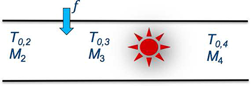
Figure 10. A schematic of a scramjet combustor tube.
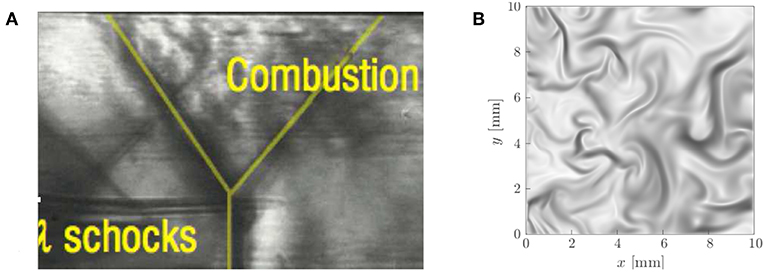
Figure 11. (A) Schlieren picture from a scramjet combustor experiment (adapted from Scherrer et al., 2016 with permission from them) and (B) numerical Schlieren from the case NP3, adapted from Doan and Swaminathan (2019a) under a Creative Commons license.
6. Summary and Conclusion
Turbulent combustion under MILD conditions has potentials to achieve ultra-low emissions, including CO2, and high thermal efficiency. Although this topic has been explored using modern experimental techniques since 1990s, a good understanding on their complexities and intricacies has evolved only in the last decade. Direct numerical simulations (DNS) have provided some detailed insights into this problem and it seems that the inception of MILD combustion cannot be described using the classical S-curve and alternative theories involving at least two chemical timescales is required. Such a theory is yet to be developed. The reaction zones under MILD conditions are observed to show the characteristics of autoignition and both premixed and non-premixed flames. The local scalar gradients controlling the various fluxes dictate the local combustion behavior. These gradients can be tailored by designing appropriate flow and scalar mixing patterns. The thermochemical and mixture conditions also play a role here. Despite the complexities of MILD reaction zones, they can be seen as homogeneous reactors locally and thus modeling approaches such as tabulated chemistry using PSR/WSR can work quite well if the CFD model and the reactor conditions are designed to be physically consistent with combustor conditions of interest. Overall, the MILD combustion could be seen as micro-volume combustion proposed in 1950s by Summerfield et al. (1955) and Shentinkov (1958). The relevance of this micro-volume combustion to supersonic combustion is shown and discussed. Further investigations using different fuels, dilution level and turbulence conditions would be useful to assess further the insights presented in this paper. Also, targeted and carefully conducted laser diagnostics of combustion under MILD condition is required.
Data Availability Statement
The datasets analyzed in this manuscript are not publicly available. Requests to access the datasets should be directed to bnMzNDFAY2FtLmFjLnVr.
Author Contributions
This paper was fully conceived and written by NS.
Funding
These works were supported by EPSRC, Cambridge Trust, Nihon Keidanren, Qualcomm European Research Studentship Fund in Technology and UKCTRF. Many of the DNS calculations were performed on the HECToR and ARCHER, UK National Supercomputing Service (http://www.archer.ac.uk) using computing time provided by EPSRC under the RAP project numbered e419 and the UKCTRF (e305). The relevance of MILD combustion to supersonic combustion was realized during my sabbatical stay at Indian Institute of Science (IISc), Bangalore, in 2018 summer, which was supported by the Centre of Excellence in Hypersonics, IISc.
Conflict of Interest
The author declares that the research was conducted in the absence of any commercial or financial relationships that could be construed as a potential conflict of interest.
Acknowledgments
The broader perspectives presented here are based on Ph.D. theses of Yuki Minamoto and Nguyen Anh Khoa Doan. Their curiosities and inquisitive nature helped me to understand the MILD combustion better and their comments on a draft of this paper are acknowledged.
Footnotes
1. ^1 ton of oil equivalent is 41.89 BJ or 11.64 MWh of energy.
References
Aminian, J., Galletti, C., Shahhosseini, S., and Tognotti, L. (2012). Numerical investigation of a MILD combustion burner: analysis of mixing field, chemical kinetics and turbulence-chemistry interaction. Flow Turbul. Combust. 88, 597–623. doi: 10.1007/s10494-012-9386-z
Bilger, R. W., Starner, S. H., and Kee, R. J. (1990). On reduced mechanisms for methane-air combustion in nonpremixed flames. Combust. Flame 80, 135–149.
Cain, T., and Walton, C. (2002). “Review of experiments on ignition and flameholidng in supersonic flow,” in 38th AIAA/ASME/SAE/ASEE Joint Propulsion Conference & Exhibit AIAA-2002-3877 (Indianapolis, IN). doi: 10.2514/6.2002-3877
Cavaliere, A., and de Joannon, M. (2004). Mild combustion. Prog. Energy Combust. Sci. 30, 329–366. doi: 10.1016/j.pecs.2004.02.003
Chen, Z., Reddy, V. M., Ruan, S., Doan, N. A. K., Roberts, W. L., and Swaminathan, N. (2017). Simulation of MILD combustion using perfectly stirred reactor model. Proc. Combust. Inst. 36, 4279–4286. doi: 10.1016/j.proci.2016.06.007
Chen, Z. X., Doan, N. A. K., Lv, X. J., Swaminathan, N., Ceriello, G., Sorrentino, G., et al. (2018). Numerical study of a cyclonic combustor under moderate or intense low-oxygen dilution conditions using non-adiabatic tabulated chemistry. Energy Fuels 32, 10256–10265. doi: 10.1021/acs.energyfuels.8b01103
Christo, F. C., and Dally, B. B. (2005). Modeling turbulent reacting jets issuing into a hot and diluted coflow. Combust. Flame 142, 117–129. doi: 10.1016/j.combustflame.2005.03.002
Dally, B. B., Karpetis, A. N., and Barlow, R. S. (2002). Structure of turbulent non-premixed jet flames in a diluted hot coflow. Proc. Combust. Inst. 29, 1147–1154. doi: 10.1016/S1540-7489(02)80145-6
de Joannon, M., Sabia, P., Cozzolino, G., Sorrentino, G., and Cavaliere, A. (2012). Pyrolitic and oxidative structures in hot oxidant diluted oxidant (HODO) MILD combustion. Combust. Sci. Technol. 184, 1207–1218. doi: 10.1080/00102202.2012.664012
de Joannon, M., Saponaro, A., and Cavaliere, A. (2000). Zero-dimensional analysis of diluted oxidation of methane in rich conditions. Proc. Combust. Inst. 28, 1639–1646. doi: 10.1016/S0082-0784(00)80562-7
De, A., and Dongre, A. (2015). Assessment of turbulence-chemistry interaction models in MILD combustion regime. Flow Turbul. Combust. 94, 439–478. doi: 10.1007/s10494-014-9587-8
Doan, N. A. K. (2018). Physical Insights of Non-Premixed MILD Combustion using DNS (Ph.D. thesis). University of Cambridge, Cambridge, United Kingdom. doi: 10.17863/CAM.32380
Doan, N. A. K., and Swaminathan, N. (2019c). Role of radicals on MILD combustion inception. Proc. Combust. Inst. 37, 4539–4546. doi: 10.1016/j.proci.2018.07.038
Doan, N. A. K., and Swaminathan, N. (2019a). Analysis of markers for combustion mode and heat release in MILD combustion using DNS data. Combust. Sci. Technol. 191, 1059–1078. doi: 10.1080/00102202.2019.1610746
Doan, N. A. K., and Swaminathan, N. (2019b). Autoignition and flame propagation in non-premixed mild combustion. Combust. Flame 201, 234–243. doi: 10.1016/j.combustflame.2018.12.025
Doan, N. A. K., Swaminathan, N., and Minamoto, Y. (2018). DNS of MILD combustion with mixture fraction variations. Combust. Flame 189, 173–189. doi: 10.1016/j.combustflame.2017.10.030
Dunn, M. J., Masri, A. R., Bilger, R. W., and Barlow, R. S. (2010). Finite rate chemistry effects in highly sheared turbulent premixed flames. Flow Turbul. Combust. 85, 621–648. doi: 10.1007/s10494-010-9280-5
Fujimori, T., Riechelmann, D., and Sato, J. (1998). “Effect of liftoff on NOx emission of turbulent jet flame in high-temperature coflowing air,” in 27th Symposium Combustion (Boulder, CO), 1149–1155. doi: 10.1016/S0082-0784(98)80517-1
Göktolga, M. U., van Oijen, J. A., and de Goey, L. P. H. (2015). 3D DNS of MILD combustion: a detailed analysis of heat loss effects, preferential diffusion, and flame formation mechanisms. Fuel 159, 784–795. doi: 10.1016/j.fuel.2015.07.049
International Energy Agency (2019). Key World Energy Statistics. Report by IEA. Available online at: www.iea.org/statistics (accessed May 13, 2019).
Kathrotia, T., Riedel, U., Seipel, A., Moshammer, K., and Brockhinke, A. (2012). Experimental and numerical study of chemiluminescent species in low-pressure flames. Appl. Phys. B Lasers Opt. 107, 571–584. doi: 10.1007/s00340-012-5002-0
Katsuki, M., and Hasegawa, T. (1998). “The science and technology of combustion in highly preheated air,” in 27th Symposium Combustion, Vol. 27 (Boulder, CO), 3135–3146.
Lee, J., Jeon, S., and Kim, Y. (2015). Multi-environment probability density function approach for turbulent CH4/H2 flames under the MILD combustion condition. Combust. Flame 162, 1464–1476. doi: 10.1016/j.combustflame.2014.11.014
Leung, T., Swaminathan, N., and Davidson, P. A. (2012). Geometry and interaction of structures in homogeneous isotropic turbulence. J. Fluid Mech. 710, 453–481. doi: 10.1017/jfm.2012.373
Li, Z., Cuoci, A., Sadiki, A., and Parente, A. (2017). Comprehensive numerical study of the adelaide jet in hot-coflow burner by means of rans and detailed chemistry. Energy 139, 555–570. doi: 10.1016/j.energy.2017.07.132
Medwell, P. R., Kalt, P. A. M., and Dally, B. B. (2007). Simultaneous imaging of oh, formaldehyde, and temperature of turbulent nonpremixed jet flames in a heated and diluted coflow. Combust. Flame 148, 48–61. doi: 10.1016/j.combustflame.2006.10.002
Minamoto, Y. (2013). Physical Aspects and Modelling of Turbulent MILD Combustion (Ph.D. thesis). University of Cambridge, Cambridge, United Kingdom.
Minamoto, Y., and Swaminathan, N. (2014a). Modelling paradigms for MILD combustion. Int. J. Adv. Eng. Sci. Appl. Math. 6, 65–75. doi: 10.1007/s12572-014-0106-x
Minamoto, Y., and Swaminathan, N. (2014b). Scalar gradient behaviour in MILD combustion. Combust. Flame 161, 1063–1075. doi: 10.1016/j.combustflame.2013.10.005
Minamoto, Y., and Swaminathan, N. (2015). Subgrid scale modelling for MILD combustion. Proc. Combust. Inst. 35, 3529–3536. doi: 10.1016/j.proci.2014.07.025
Minamoto, Y., Swaminathan, N., Cant, R. S., and Leung, T. (2014). Reaction zones and their structure in MILD combustion. Combust. Sci. Technol. 186, 1075–1096. doi: 10.1080/00102202.2014.902814
Ozdemir, I. B., and Peters, N. (2001). Characteristics of the reaction zone in a combustor operating at MILD combustion. Exp. Fluids 30, 683–695. doi: 10.1007/s003480000248
Parente, A., Malik, M. R., Contino, F., Cuoci, A., and Dally, B. B. (2016). Extension of the eddy dissipation concept for turbulence/chemistry interactions to MILD combustion. Fuel 163, 98–111. doi: 10.1016/j.fuel.2015.09.020
Pitsch, H., and Fedotov, S. (2001). Investigation of scalar dissipation rate fluctuations in non-premixed turbulent combustion using a stochastic approach. Combust. Theor. Model. 5, 41–57. doi: 10.1088/1364-7830/5/1/303
Prisell, E. G. (2006). The Feasibility of the Scramjet; An Analysis Based on First Principles. Available online at: https://www.icas.org/ICAS_ARCHIVE/ICAS2006/ABSTRACTS/530.HTM
Sahni, V., Sathyaprakash, B. S., and Shandarin, S. F. (1998). Shapefinders: a new shape diagnostic for large-scale structure. Astrophys. J. 495, L5–L8. doi: 10.1086/311214
Scherrer, D., Dessornes, O., Ferrier, M., Vincent-Randonnier, A., Moule, Y., and Sabelnikov, V. (2016). Research on supersonic combustion and scramjet combustors at ONERA. Aerospacelab J. 11, 1–20. doi: 10.12762/2016.AL11-04
Shentinkov, E. S. (1958). “Calculation of flame velocity in turbulent stream,” in Symposium (International) on Combustion, Vol. 7 (Oxford, UK), 583–589.
Sidey, J. A. M., and Mastorakos, E. (2015). Visualization of mild combustion from jets in cross-flow. Proc. Combust. Inst. 35, 3537–3545. doi: 10.1016/j.proci.2014.07.028
Smooke, M. D., and Giovangigli, V. (1991). “Formulation of the premixed and nonpremixed test problems,” in Reduced Kinetic Mechanisms and Asymptotic Approximations for Methane-Air Flames; Vol. 384 of Lecture Notes in Physics, ed M. D. Smooke (Berlin; Heidelberg: Springer), 1–28. doi: 10.1007/BFb0035362
Sorrentino, G., Sabia, P., Bozza, P., Ragucci, R., and de Joannon, M. (2017). Impact of external operating parameters on the performance of a cyclonic burner with high level of internal recirculation under MILD combustion conditions. Energy 137, 1167–1174. doi: 10.1016/j.energy.2017.05.135
Sorrentino, G., Sabia, P., de Joannon, M., Cavaliere, A., and Ragucci, R. (2016). The effect of diluent on the sustainability of MILD combustion in a cyclonic burner. Flow Turbul. Combust. 96, 449–468. doi: 10.1007/s10494-015-9668-3
Summerfield, M., Reiter, S. H., Kebely, V., and Mascolo, R. W. (1955). The structure and propagation mechanism of turbulent flames in high speed flow. J. Jet Propulsion 25, 377–384.
Suzukawa, Y., Sugiyama, S., Hino, Y., Ishioka, M., and Mori, I. (1997). Heat transfer improvement and NOx reduction by highly preheated air combustion. Energy Convers. Manage. 38, 1061–1071.
van Oijen, J. A. (2013). Direct numerical simulation of autoigniting mixing layers in MILD combustion. Proc. Combust. Inst. 34, 1163–1171. doi: 10.1016/j.proci.2012.05.070
Keywords: MILD combustion, Scramjet, DNS, morphology, inception, S-curve
Citation: Swaminathan N (2019) Physical Insights on MILD Combustion From DNS. Front. Mech. Eng. 5:59. doi: 10.3389/fmech.2019.00059
Received: 28 May 2019; Accepted: 19 September 2019;
Published: 02 October 2019.
Edited by:
Mara de Joannon, Istituto di Ricerche sulla Combustione (IRC), ItalyReviewed by:
Shiyou Yang, Ford Motor Company, United StatesKhanh Duc Cung, Southwest Research Institute, United States
Copyright © 2019 Swaminathan. This is an open-access article distributed under the terms of the Creative Commons Attribution License (CC BY). The use, distribution or reproduction in other forums is permitted, provided the original author(s) and the copyright owner(s) are credited and that the original publication in this journal is cited, in accordance with accepted academic practice. No use, distribution or reproduction is permitted which does not comply with these terms.
*Correspondence: N. Swaminathan, bnMzNDFAY2FtLmFjLnVr